Constraint Objects Integrating Constraint Definition and Graphical ...

Constraint Objects { Integrating Constraint De
nition and Graphical Interaction Ching-yao Hsu Beat Bruderlin UUCS-92-038

Department of Computer Science University of Utah Salt Lake City, UT 84112 USA November 23, 1992

Abstract: This paper describes the implementation of a new constraint-based tech-

nique for direct manipulation in interactive CAD, which will simplify the design process, especially in the early stages. We introduce so called Constraint Objects and Parameter Objects which constitute an object-oriented view on constraints. They serve to simulate the mutual degrees of freedom between objects for which a geometric relation (distance, angle, parallel, congruence, etc.) has been de ned. A 2-D pro le editor has been realized for interactively constructing lines and circles in various ways. Each construction operation, implicitly de nes constraints to capture the intent of the operation. These constraints are represented by corresponding parameter objects and constraint objects. A constraint solver is applied to rewrite the set of constraints into its normal form if necessary. Finally, the resulting parameter-constraint-regular-object network serves to simulate the degrees of freedom of geometric objects during interactive dragging manipulations, and to make sure the existing constraints are not violated by subsequent operations.

1 Introduction Conventional modeling systems do not support the free dimensioning of geometric objects by means of constraints, but require users to construct them by a sequence of geometric operations. Mechanical parts designed by such a CAD system are represented as xed geometry the geometric design part is completely separated from other design criteria. It is dicult for a user to add information under a dierent view, later on. Changing a part may inadvertently violate previous design decisions.

Geometric constraints have proven useful for interactive geometric design (see bibliography for references). The idea is to specify shape by constraints such as distances, angles, etc. and use a constraint solver to derive the shape from such a speci cation. A clear drawback of a constraint based approach is that it is not intuitive for complex examples. It is extremely dicult for a designer to come up with a complete and consistent set of constraints. Often we encounter over and under speci ed parts simultaneously that are hard to resolve in a speci cation. This is addressed, e.g. in 14]. Also constraint solving is very dicult, even if the speci cation is consistent. Most constraint based systems use numerical techniques (relaxation, Newton iteration) which can theoretically solve problems that don't have a closed form algebraic or geometric solution on the other hand numerical techniques have convergence problems that make them very unpredictable. We investigated ways of specifying geometric objects by geometric constraints, and developed a new mechanism for symbolic geometric constraint solving. Constraints are represented symbolically as predicates over points. A rewrite rule mechanism seeks to match the left hand side of a rule with a subset of the constraints. If a rule applies some of the predicates are replaced by new, simpler ones, and a construction operation is applied to satisfy these constraints simultaneously 7], 8]. In 21], 22] we have shown that object-oriented graphical interaction can be integrated naturally with constraint de nition and constraint solving for 3-d assembling of mechanical parts. Other approaches that integrate constraint de nition and interactive modeling can be found, for instance in 10], 13], 17], 18], 19], and 23]. Constraints can also be used to communicate un nished design, etc. (constraints are part of the model data). This solves in part the problem of later modi cations being consistent with previous ones, allowing one to communicate ideas between dierent departments of the design oce during the early design process. In this paper we continue our eorts to integrate constraint solving techniques with graphical object-oriented interaction by introducing so called constraint objects.

2 Constraint Objects The role of the constraint objects is to simulate relative degrees of freedom between constrained objects. The types of constraint objects supported in here are chosen to be compatible with the types of constraints used in the symbolic geometric constraint solver, described in 8]. pos(A, Pos): The position of point A by a symbolic expression Pos. dist(A,B, d): The distance between points A and B is de ned by d. slope(A,B, s): The slope of the line through A and B is s. vector(A,B, v): Point B is oset from point A by a vector v. angle(A,B,C, Alpha): The angle between line AB and line BC is Alpha. In the following sections the function of the constraint objects is described in some detail.

d

P1 s

P2

P2 (b) slope(P1,P2, s)

(a) dist(P1,P2, d)

P1 P2

P1

P1 alpha

alpha P3 (c) angle(P1,P2,P3, alpha)

P2

P3 (d) angle(P1,P2,P3, alpha)

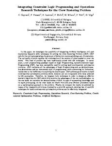
Figure 1: The various degrees of freedom for dierent constraint objects

2.1 The Eect of an Individual Constraint A point that is constrained by one of the above constraints has a degree of freedom determined by the type of constraint and the degrees of freedom of the other points constrained by the same constraint. Figure 1 shows various cases for the degree of freedom of a point related to other points by one constraint, assuming that the other points remain xed. For the constraints introduced here, the loci de ned by a constraint object are circles and straight lines. Table 2.1 determines the degrees of freedoms of a point attached to one constraint, assuming that one other point attached to the same constraint has a degree of freedom of 2, 1, or zero, respectively.

constraint type o.p. has dof 0 o.p. has dof 1 o.p. has dof 2 position 0 na na vector 0 1 2 slope 1 2
2 angle 1 2
2 distance 1 2
2 Table 1: the degree of freedom of a point to which a constraint has been attached (assuming that another point attached to that constraint has 0, 1, or 2 dofs) intersecting two constraints resulting dof 2^2 2 2^1 1 2^0 0 1^1 0 1^0 0 0^0 0 Table 2: multiple constraints attached to one point with dierent dofs here's how they add

2.2 Multiple Constraints Multiple constraints attached to the same point further restrict this point's degree of freedom. Table 2.2 shows the eect of two constraints attached to the same point each determining a degree of freedom, taken individually. From this information, we are now going to derive a recursive algorithm, that can determine for any point P that is directly or indirectly constrained to other points by many constraints, what its degree of freedom is, and which other points need to be changed, when P is changed within its degree of freedom. The way the function is used, is that one requests a degree of freedom for a point P, by calling rqdofP(P, dof), where dof = 2, 1, or 0. The function then checks whether that can be achieved, and which other points are involved, and how. In 2-D we can start requesting a degree of freedom of 2, i.e. we want to move the point freely, but other points have to react to the changes. If there is no way that point P can be moved freely, we can try to request a degree of freedom of 1. If successful the point can be moved along a curve. If it fails, the point cannot be moved at all. The algorithm is subdivided in 2 recursive functions, mutually calling each other. procedure rqdofP(P, dof) begin

(*requests a degree of freedom for a point *)

find the set C of constraints attached to P if dof = 2 then (* all the dofs requested from all the constraints attached to P must be 2 *) for each constraint C1 in C do rqdofC(P, 2, C1) if dof = 1 then begin pick some constraint C1 and call rqdofC(P, 1, C1) for each constraint C2 in C where C2 != C1 do rqdofC(P, 2, C2) end if dof = 0 then return end ----------------------------------------------Procedure rqdofC(P, dof, Constr) (* requests a degree of freedom from a single constraint *) begin if dof = 2 then IF Constr = pos(P,_) then fail IF Constr = vector(P,P1,_) or Constr = vector(P1,P,_) then rqdofP(P1, 2) IF Constr = slope(P,P1,_) or Constr = slope(P1,P,_) then rqdofP(P1, 1) IF Constr = dist(P,P1,_), or Constr = dist(P1,P,_) then rqdofP(P1, 1) IF Constr = angle(P,P1,P2,_), or Constr = angle(P1,P,P2,_), or Constr = angle(P1,P2,P,_) then rqdofP(P1, 1) rqdofP(P1, 0) or rqdofP(P2, 1) rqdofP(P2, 0) else if dof = 1 then IF Constr = pos(P,_) then fail IF Constr = vector(P,P1,_) or

Constr IF Constr or Constr IF Constr or Constr IF Constr or Constr or Constr

= vector(P1,P,_) then rqdofP(P1, 1) = slope(P,P1,_) = slope(P1,P,_) = dist(P,P1,_),

then rqdofP(P1, 0)

= dist(P1,P,_) then rqdofP(P1, 0) = angle(P,P1,P2,_), = angle(P1,P,P2,_),

= angle(P1,P2,P,_) then rqdofP(P1, 0) rqdofP(P1, 0) or rqdofP(P2, 0) rqdofP(P2, 0) else if dof = 0 then always succeed end

3 Evaluating the Degrees of Freedom 3.1 Phase 1: Finding the dependency graph To illustrate the eect of the algorithms we can depict the relationships by directed, acyclic hyper-graphs. A node in the graph shows a point together with its degrees of freedoms. An arc in the graph represents a constraint and is labeled with the degrees of freedoms associated with the constraint. Looking at it in another way, a node corresponds to a call of rqdofP(P, dof), and an arc to a call rqdofC(P, dof, C). When we try to move a point, a dependency graph is established this way. An example is shown in Figure 2. For a certain constraint network, there might be several valid dependency graphs associated with it. This is reected by the non-deterministic formulation of the algorithms, using logical 'or' between statements. We therefore need to have a criterion for selecting an 'optimal' graph among them. Ideally, we will expect the move to aect as few other points as possible. Or in terms of the graph, we would like to minimize the levels of the graph. As a consequence, the search strategy we adopt is breadth- rst search together with backtracking.

3.2 Phase 2: Evaluating the geometric solution After determining the degree of freedom of a point we need to evaluate the amount of change in the positions of the points involved that need to be adjusted. The design of this algorithm

B x

y C

A dist(A,B, x) dist(B,C, y)

(a) The constraint network

rqdof(B, 2) rqdofC(B, 1, alpha) rqdofP(A, 1) rqdofC(B, 2, beta) rqdofP(C, 1) (d) another calling sequence

rqdofP(B, 1) rqdofC(B, 1, alpha) rqdofP(A, 0) rqdofC(B, 2, beta) rqdofP(C, 1) (b) The calling sequence

B1 x1

y2

A0

C1

(c) The dependency graph

B2 x2

y2

A1

C1

(e) another dependency graph

Figure 2: The constraint network and its dependency graph

emphasize on eciency so that user can get fast feedback from display. As a consequence, iterative methods are deliberately avoided. We realize that it is not possible for the user to predict where to drag the point when it has one degree of freedom. Naturally, we the user only speci es the amount and the direction of the change rather than the point following the cursor. Note also that once the dependency graph is established, we don't need to construct the graph again each time we try nd a new position. Instead, we can use this graph to evaluate the new dimensioning of the network as many times as we want. However, there is no guarantee that a geometric solution will exist even if a dependency graph does exist. For instance, when one tries to drag the point too far or in an impossible direction. In these case, this algorithm will do nothing to the points so that the constraints are still maintained. This algorithm uses the graph produced by phase 1 and determines the position of the constrained points in the graph by a set of rules which governs the order and the means of the evaluation. Depending on the purposes, the rules are further divided into three categories, namely seeding rules, propagation rules, and evaluation rules. 3.2.1 Seeding rules

The seeding rules to some extent determine the order in which the points need to be changed. We have two rules used respectively for one and two degrees of freedom we request from the point changed. rule 1: One degree of freedom In the simplest cases, the locus of the point dragged will only depend on the constraint which we request one degree of freedom from, ie. all the other points con ned by the same constraint remain unchanged, then we can start with this point. On the other hand, if some of the other points constrained by the same constraint request some degrees of freedom to facilitate the change, we need to recurse down the arc to nd the position of those points rst. rule 2: Two degrees of freedom If we request two degrees of freedom from the point we dragged the new position is not depending on updates further down in the dependency graph, so we can directly update this point, and then recurse. 3.2.2 Propagation rules

The propagation rules determine how the changes are propagated up in the dependency graph, once they are made. The basic principle behind propagation rules is that a one degree of freedom intersecting with another one degree of freedom yields zero degree of

freedom. Consequently, if a point satis es one of the following conditions, it can re, and the position can be evaluated. condition 1: a point is constrained by a set of constraints and at least two of them give one degree of freedom (ie, the other constraints yield two degrees of freedom). condition 2: a point is constrained by only one constraint which yields one degree of freedom. Once the position of a point is determined, it has only zero degrees of freedom. We need to update the graph to reect this change. We will rst mark the point as having zero degree of freedom and then mark all the constraints attached as having one less degree of freedom. Note that condition 1 allows points with more than two constraints each yielding one degree of freedom to re. 3.2.3 Evaluation rules

Depending on the condition which causes a point to re, we have dierent evaluation rules. If the point res by the rst seeding rule, the new position of the point will be function of the constraint giving one degree of freedom and a vector propagated from the root. If we request one degree of freedom from the point to be dragged, we can interpret the graph as an equation which gives the locus of the point dragged. In order to solve this simultaneous systems of constraints, therefore, we will have to provide one more equation. In an interactive environment, we normally expected the magnitude and direction of the change correspond to the magnitude and direction of the dragging motion. In other words, we want the new position of the point to be a function of how much and in which direction the user drags the point. If the point res by condition 1, we can evaluate the position of the point by nding the intersection of the loci determined by those constraints which give one degree freedom. For example, if a point is constrained by a distance constraint giving one degree of freedom, then the locus of the point is a circle with the center being the other point constrained by the same distance constraint and radius being the distance between the two points. Therefore if a point is constrained by two distance constraints each giving one degree of freedom, we can evaluate the position of the by intersecting two circles. Sometimes, there will be more than one solution. In this circumstance, we need to pick one position among them by some criterion, for example, the point which is nearest to the old position. Other times, there will be no intersection at all and a solution is not possible although phase one produces a valid graph. Therefore the algorithm will fail keeping all the points involved unchanged. On the other hand, if the point has only one constraint attached, we know that the point will be determined by the locus determined by the constraint. But we still need to pick one point. We propose two methods to pick the point. The rst method is to use the old position as a reference, and then nd the point on the locus which is nearest to the

old position. Alternatively, we can propagate the vector of change of the known point as a reference. If a point has only one constraint, it can use this vector to evaluate its new position.

4 Changing the Parameter of a Constraint We can extend the previous algorithm to handle the case when user picks a constraint and speci es a new parameter for that constraint. Under these circumstances, we rst remove temporarily the constraint from the constraint network, and then request degree of freedom one from one point, and also x the other points constrained by the constraint. Next, we construct the dependency graph as before. We will then try to nd a new solution for the graph in such a way that the newly speci ed parameter of the said constraint is met. In order to achieve this, we need an iterative method which will take an initial guess on the seeding point, propagate through the whole graph, calculate the oset between the new value and the speci ed value for the said constraint, and then repeat this process until the oset is under a threshold.

5 Parameter Objects The idea of constraint objects has been extended to also facilitate congruence relations, parallelism, encidence, etc. In our system we realize such relations by introducing so called parameter objects. In short, a constraint object, for instance a distance constraint, does not carry the value of the distance itself, but instead refers to a parameter object. This way, two distance constraint objects can share the same parameter object. A Boolean ag associated with the parameter object indicates whether this value is xed (meaning that the constraint object is a distance constraint) or variable (meaning that two or more distances are congruent) and just signi es the current value. The algorithms described above which determine the degree of freedom of points, and the ones that evaluate the changes during dragging operations, need to be modi ed to allow for this extra degree of freedom each constraint object may have. During dragging operations the parameter value may be updated when an additional degree of freedom is requested from a constraint object. For all other constraint objects this value is then considered xed, so that the constraint relation is maintained. Parallel lines, or collinear lines, for instance, may be realized by two slope constraints sharing the same variable parameter. Coincident points are realized by two position constraint objects sharing the same parameter.

Figure 3: A pro le created with the editor

6 A Prole Editor with Implicit and Explicit Constraints To provide a comprehensive example of the integration of graphical interaction, constraint solving and constraint objects we started implementing a 2-d pro le editor. In this implementation 2-d pro les are de ned by circle and line segments. In nite lines and full circles can be de ned as references, to simplify interaction. 2-d pro les can be de ned by concatenating circle and line segments enclosing an area. Figure 3 shows an example of a pro le de ned by intersecting lines and circles, creating lines tangent to circles, parallel or perpendicular to other lines, or as angle bisectors, etc. For every construction operation we automatically create implicit constraints that maintain the characteristics of the operation under later changes. For instance, a line constructed to be tangent to two circles needs to remain tangent when the radius or position of the circles is changed, or the line itself is changed. Also, explicit constraints can be de ned to specify distances, angles, etc. Whenever an explicit constraint is added the constraint solver is run to check its validity and to satisfy simultaneous constraints. The constraint solver itself is based on geometric rewrite rules that can simplify the constraint graph. This paper does not describe the symbolic geometric constraint solver, instead, we refer to 8]. All the implicit and explicit constraints are represented as constraint objects, as described above. Objects can be manipulated directly by dragging them within their degree of freedom speci ed by the attached constraint objects. In the example shown in Figure 4 (a), the two circles and the tangent line are created by construction operations which in turn de ne implicit constraints, ie. the two (right-) angle constraints, to capture the intent of the operation as shown in Figure 4 (b). We later x the centers of the two circles as well as the radius of the left circle by attaching explicit constraints

to them (which are depicted as solid points and solid circle, respectively). Suppose now we try to change the tangent line by dragging point C. The rst phase of the algorithm will produce a dependency graph as shown in Figure 4 (d). Then using the seeding rule, point B is picked as the rst point to evaluate. From the graph, point B is constrained by the distance constraint dist, and therefore it will be on the circle with point A as the center and the distance between point A and point B as the radius. We then determine the new position of point B corresponding to the magnitude and the direction of the dragging motion. Once the new position point B is obtained, point C can be unique determined by the two angle constraints. Figure 4 (e) show one instance of the evaluation phase. Figure 5 shows another example where a line segment with xed length is attached to two lines with xed slope.

7 Conclusion It is crucial to give adequate feedback to the user in the early design phases, when most parts of a design are not yet fully constrained. Constraint objects allow for a uniform, objectoriented representation of constraints by graphical objects which allows for an interactive simulation of under constrained objects and their internal degrees of freedom. Generally speaking, the capability to specify constraints in an iterative CAD makes manipulation and modi cation much easier because system takes most of the responsibilities to maintain consistency. In addition, we provide the capability to simulate the degrees of freedom of under-constrained networks of constraints which enable user to draft in a less restricted way in the early design stage. With constraint objects we completed the framework for interactive geometric modeling that integrates object-oriented manipulation of objects, declarative (relational) de nition by constraints (using a constraint solver) and procedural de nition (using geometric construction operations).

8 Acknowledgments This work has been supported, in part, by NSF grants DDM-89 10229 and ASC-89 20219, and a grant from the Hewlett Packard Laboratories. All opinions, ndings, conclusions, or recommendations expressed in this document are those of the authors and do not necessarily reect the view of the sponsoring agencies.

References 1] I. Sutherland \Sketchpad, A Man-Machine Graphical Communication System", Ph.D. thesis, MIT, January 1963.

C

C A

D B

Pos(A, Pos1) alpha dist B

beta

(b)

(a)

C1

beta1 C A

D0

B

Pos(D, Pos2) angle(A,B,C, alpha) angle(B,C,D, beta) dist(A,B, dist)

B0

D

B1

alpha2 B1 A0 combine B0 and B1 together

dist1 A0 (c)

(d)

alpha C A B dist

beta D

(e)

Figure 4: A line tangent to two circles

t dist

Pos(A, Pos2) B B'

Pos(D, Pos1) C' C

C1 s

slope(A,B, s) slope(C,D, t) dist(B,C, dist) (a)

t1 D0

s2 B1 dist1 A0 (b)

Figure 5: Line segment attached to two slots 2] B. Aldefeld \Variation of Geometries based on a geometric reasoning method", in Computer-Aided Design Vol. 20, No. 3, 1988 3] L. A. Barford \A Graphical, Language-Based Editor For Generic Solid Models Represented By Constraints", Cornell University, May 1987. 4] E. A. Bier \Snap Dragging in 3-dimensions", in Proceedings of the 1990 Symposium on Interactive 3-d Graphics , 1990. 5] B. Borning \The Programming Language Aspects of ThingLab, a Constraint-Oriented Simulation Laboratory", ACM Toplas Vol. 3, No. 4, Oct 1981. 6] G. L. Steele Jr. and G. J. Sussman \CONSTRAINTS - A language for expressing almost-hierarchical descriptions", Articial Intelligence pp1-39, Jan 1980. 7] Bruderlin, B. \Rule-Based Geometric Modelling", Ph.D. thesis, ETH Zurich, Switzerland, 1987, Published by vdf-Verlag, Zurich, 1988. 8] Bruderlin, B. \A rewrite-rule system for solving geometrical problems symbolically", To be published by Theoretical Computer Science , 1993. 9] T. W. Fuqua \Constraint Kernels: Constraints and Dependencies in a Geometric Modeling System", University of Utah, Aug, 1987. 10] M. Gleicher \Integrating Constraints and Direct Manipulation", Symposium on 3-d Interactive Graphics, 1992.

11] D. Gossard and R. Zuffante \Representing Dimensions, Tolerance and Features", IEEE Computer Graphics and Applications , 1988. 12] J. Hopcroft, D. Joseph and S. Whitesides \Movement Problems for 2dimensional Linkages", SIAM Journal of Computation , Vol. 13, No. 3, Aug. 1984. 13] G. Kramer \Using Degrees of Freedom Analysis to Solve Geometric Constraint Systems" in Proceedings of the 1991 ACM/SIGGRAPH Symposium on Solid Modeling Foundations and CAD/CAM Applications , 1991. 14] R. Light and D. Gossard \Modi cation of geometric models through variational geometry", Computer Aided Design , Vol. 14, No. 4, Jul. 1982. 15] G. Nelson \Juno, a constraint-based graphics system", ACM SIGGRAPH , 1985, pp.235-243. 16] J. C. Owen \Algebraic Solution for Geometry from Dimensional Constraints", in Proceedings of the 1991 ACM/SIGGRAPH Symposium on Solid Modeling Foundations and CAD/CAM Applications , 1991. 17] Roller, D. A system for interactive variation design. In: Geometric Modelling for Product Engineering Wozny M., Turner J., Preiss K., (eds), North Holland, 1989. 18] D. Roller \An Approach to Computer-Aided Parametric Design", Computer-Aided Design , Vol 23. No. 5, June 1991 19] J. R. Rossignac \Constraints in Constructive Solid Geometry", Interactive 3-d Graphics , 1986. 20] H. Suzuki, H. Ando, and F. Kimura \Geometric Constraints and Reasoning for Geometrical CAD", Computers and Graphics , Vol. 14, No. 2, 1990. 21] W. Sohrt and B. Bruderlin \Interacting with Constraints in 3-d", in Proceedings of the 17th ACM Conference on Advances in Design and Manufacturing , Austin Texas, January 1991. 22] W. Sohrt and B. Bruderlin \Interaction with Constraints in 3-d Modeling", in Proceedings of the 1991 ACM/SIGGRAPH Symposium on Solid Modeling Foundations and CAD/CAM Applications , June 1991. International Journal of Computational Geometry and Applications , 1991. 23] Maarten van Emmerik \Interactive design of parameterized 3-d models", Ph.D. Thesis, 1990. 24] A. Witkin, K. Fleischer, and A. Bar \Energy Constraints on Parameterized Models", Computer Graphics , Vol. 21, Jul 1987.

25] Jan Wolter and P. Chandrasekaran \A Concept for a Constraint Based Representation of Functional and Geometric Design Knowledge" in Proceedings of the 1991 ACM/SIGGRAPH Symposium on Solid Modeling Foundations and CAD/CAM Applications , June 1991.