Constructing neural networks for multiclass

IEEE TRANSACTIONS ON SYSTEMS, MAN, AND CYBERNETICS—PART B: CYBERNETICS, VOL. 29, NO. 3, JUNE 1999

445

Constructing Neural Networks for Multiclass-Discretization Based on Information Entropy Shie-Jue Lee, Mu-Tune Jone, and Hsien-Leing Tsai

Abstract— Cios and Liu [5] proposed an entropy-based method to generate the architecture of neural networks for supervised two-class discretization. For multiclass discretization, the inter-relationship among classes is reduced to a set of binary relationships, and an independent two-class subnetwork is created for each binary relationship. This twoclass-based method ends up with the disability of sharing hidden nodes among different classes and a low recognition rate. We keep the interrelationship among classes when training a neural network. Entropy measure is considered in a global sense, not locally in each independent subnetwork. Consequently, our method allows hidden nodes and layers to be shared among classes, and presents higher recognition rates than the two-class-based method. Index Terms— Delta rule, entropy function, hyperplanes, neural networks, simulated annealing.

I. INTRODUCTION Using backpropagation algorithms [15], [11] in implementing multilayer neural networks, we are confronted with the problem of determining the number of hidden layers and the number of nodes in each hidden layer. Conventionally, a trial-and-error method must be used to find the proper neural network architecture for a given problem. To overcome this difficulty, several approaches have been proposed recently to generate the architecture of neural networks. Kung and Hwang [10] used the algebraic projection analysis to specify the size of hidden layers. Fahlman and Lebiere [6] proposed cascade-correlation neural networks in which new hidden nodes are added dynamically by maximizing a correlation measure. Goodman et al. [8] used a J-measure to derive from training data a set of rules which are then used to construct a neural network. Nadal [16], Bichsel and Seitz [2], and Cios and Liu [5] used entropy to determine the number of hidden layers and the number of nodes in each hidden layer. The method proposed by Cios and Liu [5] applied an entropy measure similar to that used in ID3 [19], [7] to generate neural network architectures. However, the method is for the construction of neural networks for two-class problems. For multiclass problems, the inter-relationship among classes is reduced to a set of binary relationships. Each binary relationship treats the data points of the underlying class to be positive examples, and all the data points of the other classes as negative examples. An independent two-class subnetwork is created for each binary relationship, as shown in Fig. 1 where K is the number of classes. Entropy is considered locally in each subnetwork. This two-class-based generation method ends up with a network in which hidden nodes in subnetworks are not shared. Furthermore, because of the reduction of the global inter-relationship into local binary relationships, networks obtained by this method have a low recognition rate. We keep the inter-relationship among classes Manuscript received December 22, 1995; revised November 10, 1996 and July 10, 1998. This work was supported by the National Science Council under Grants NSC-82-0408-E-110-139 and NSC-83-0408-E-110-004. A preliminary version of this paper appeared was presented at the International Symposium on Artificial Neural Networks, Tainan, Taiwan, R.O.C., December 1994. This paper was recommended by Associate Editor P. Borne. The authors are with the Department of Electrical Engineering, National Sun Yat-Sen University, Kaohsiung, Taiwan 80424, R.O.C.. Publisher Item Identifier S 1083-4419(99)02297-9.

Fig. 1. Two-class-based multiclass network.

when training a neural network. Entropy measure is considered in a global sense, not locally in each independent subnetwork. As a result, our method allows hidden nodes and layers to be shared among classes, and presents higher recognition rates than the two-class-based method. In this paper, as in [5], we assume that one output node is created for each class. If an input belongs to a certain class, then the output node representing the class will be activated and the other output nodes will be deactivated. The rest of the paper is organized as follows. Section II introduces entropy measures for deriving hyperplanes for hidden and output neurons, and explains why we need different measures. Section III develops delta rules which guide the finding of optimal hyperplanes in an efficient manner, with the help of simulated annealing [12], [1]. Section IV presents the procedures for building the whole neural net, given a set of training data. Finally, Section V provides experiment results and compares our method with Cios and Liu’s two-class-based method. II. ENTROPY MEASURES FOR FINDING HYPERPLANES Suppose we have a set D of training examples with K classes 1 1 1 ; CK : Each example in D is represented by the following data structure:

C1 ;

struct example f ~ v : an array of attribute values (real numbers);

g

c: c

2f

C1 ; C2 ;

111

; CK

g;

:

For convenience, we will use e:~v to represent all attribute values of the example e; e:vj to represent the attribute value vj of e; and e:c to represent the category of e: Let S be a subset of D: The class entropy of S is defined as I (S )

P (Ci ; S )

=

0

K k=1

P (Ck ; S ) log2 P (Ck ; S ):

is the proportion of examples in

namely, P (Ck ; S )

=

S

that belong to class

jf 2 j = k gj j j e

S e:c

C

S

where jX j denotes the number of elements in into a partition of I sets S1 ; 1 1 1 ; SI ; and

1083–4419/99$10.00  1999 IEEE

Ci ;

X:

Let

S

=

S

be divided Si : For

[iI=1

446

IEEE TRANSACTIONS ON SYSTEMS, MAN, AND CYBERNETICS—PART B: CYBERNETICS, VOL. 29, NO. 3, JUNE 1999

convenience, we denote such a partition as fSi gIi=1 : Then the information entropy of the partition is defined as

I f i giI=1 ) = jf j giIj j i=1 i i=1 S

E( S

S

i)

I (S

(1)

according to [5] and [7]. Clearly, the value of E (fSi giI=1 ) is nonnegative and is zero when all the data points in each Si ; 1  i  I ; belong to the same class. I Let a hyperplane H (w; ~ ~ x) refine a partition fSi gi=1 to an0 I other partition fSi gi=1 : For convenience, we use the notation 0 I fSi giI=1 =H (w; ~ ~ x) for fSi gi=1 to represent explicitly the effect of the hyperplane. The addition of the hyperplane results in the following entropy gain:

f i giI=1 ( )) I = (f i gi=1 ) 0 (f I = (f i gi=1 ) 0 (f

Gain (

S

(a) Fig. 2. Refining with different hyperplanes.

; H w; ~ ~ x

E

S

E

S

i giI=1 ) I E Si gi=1 =H (w; ~ ~ x)): which Gain (fSi giI=1 ; H (w; ~ ~ x)) E

S

Also, we have

0

0

I (d1 )

The hyperplane H (w; ~ ~ x) for is maximal amongst all the candidate hyperplanes is selected as the best hyperplane to refine fSi giI=1 : Since E (fSi giI=1 ) is a constant for all candidate hyperplanes, the best hyperplane to be selected minimizes the information entropy E (fSi giI=1 =H (w; ~ ~ x)): Since hidden neurons and output neurons have different responsibilities, we use different information entropy functions to generate hyperplanes for them. The information entropy function for hidden neurons enables us to find as few hyperplanes as possible in refining a given partition, while the information entropy function of output neurons enables us to find a hyperplane which separates a class from the other classes if the separation is possible. For convenience, we K to denote these two entropy functions, respectively. use EH and EO

H (fdr gr2=1 =H2 ) =

E

r

and

r

d

r = dr [ dr ;

d

0

1

r = Nr

N

where Nr = jdr j; Nr1 = jd1r j; and from (1) we have

N

+N

N

= 10;

1

= 3;

0

N1

1

N2

N

0

N

I (d2 )

N1

0

= 3;

N1

1

0

I (d1 )

+

N2 N

1

I (d2 )

= 0:675:

1

= 3;

1 = 0:918; I (d1 ) = 0; 2 0 ( d =1 =H2 ) = 0:275:

N2

= 2;

0

=2

N2

1

I (d2 )

0

= 0;

I (d2 )

= 0;

H f r gr Since EH (fdr gr2=1 =H2 ) is smaller than EH (fdr gr2=1 =H2 ); H2 is a

0

rk = fe 2 dr je:c = Ck g 1 drk = fe 2 dr je:c = Ck ^ H (w; ~ e:~ v ) > 0g 0 drk = fe 2 dr je:c = Ck ^ H (w; ~ e:~ v )  0g 1 1 0 0 Nrk = jdrk j; Nrk = jdrk j; Nrk = jdrk j: Then the

and relations hold:

K =

k=1

1

rk

d

r0 = dr 0

;

K

d

1 ; rk

d

k=1 0 1 = drk 0 drk ; rk

And we have

r1) = 0

(2)

r0) = 0

I (d

K k=1 K k=1

1

K

N

r

N

r0 = Nr 0

N

d

I (d

= 4:

H2 :

d

r

N2

0

better choice for refinement than Let

0

= 0;

0

N2

0

r

r0 = jd0r j: and Nr0 = jd0r j: Then

= 3;

N

I (d1 )

0

N1

0

N1

+

and

1

with N = jDj: For example, suppose a data set with three classes is already divided in two subsets, d1 and d2 ; by a hyperplane H1 ; as shown in Fig. 2. Consider the refinement obtained by the candidate hyperplane H2 ; as shown in Fig. 2(a). We have N

1

= 10;

d

~ ~ x)) H (fdr grR=1 ) = EH (fdr grR=1 =H (w; R N1 r I (dr1) + Nr0 I (dr0) = N r=1 N

E

1

I (d1 )

Consider another refinement obtained by the candidate hyperplane 0 H2 ; as shown in Fig. 2(b). Now we have

are disjoint, the following relations hold: 1

1

N1

+

~ e:~ v ) > 0g r1 = fe 2 dr jH (w; 0 dr = fe 2 dr jH (w; ~ e:~ v )  0g:

d

;

0 I (d2 ) = 1:

Therefore

d

Since

:

1 I (d2 ) = 0;

0

Assuming a data set D has already been divided into a partition fdr gRr=1 : Suppose we want to refine the partition fdr grR=1 by adding 0 R one more hyperplane H (w; ~ ~ x): Let the refinement be fdr gr =1 which, R as before, is written as fdr gr=1 =H (w; ~ ~ x): The hyperplane to be selected is to minimize EH (fdr0 grR=1 ): Since each dr0 is obtained by 0 R some dj refined by H (w; ~ ~ x); we can express fdr gr =1 in a more R desirable way. Let each set dr in fdr gr=1 be divided by H (w; ~ ~ x) into two subsets: dr1 which is on the positive-side of H (w; ~ ~ x); and 0 ~ ~ x): That is dr which is on the nonpositive side of H (w;

0

0[ 13 log2 13 + 23 log2 32 + 03 log2 30 ] = 0 918

=

1 I (d1 ) = 0;

E

A. Information Entropy Function for Hidden Neurons

1

(b)

=

k=1

N

following

1 rk

K N

1 rk

k=1 0 1 = Nrk 0 Nrk : rk

1 rk 1 log2 Nr

N

1 rk 1 Nr

N

0 0 Nrk rk log2 0 0 Nr Nr

N

:

Therefore, (2) becomes

~ ~ x)) H (fdr grR=1 =H (w; R K 1

E

=

0

N

r=1 k=1

N

1 log2 rk

1 rk 1 Nr

N

+N

0 log2 rk

0 rk 0 Nr

N

IEEE TRANSACTIONS ON SYSTEMS, MAN, AND CYBERNETICS—PART B: CYBERNETICS, VOL. 29, NO. 3, JUNE 1999

which is

447

So

~ ~ x)) H (fdr gRr=1 =H (w;

E

R K

01

=

I (D

1

N

r=1 k=1

N

Nrk 1 log2 rk K 1 N rk k =1

1 ) rk 0 Nrk

(N

1

0

)=

0

NK

)=

0

NK

0

N

NK

0 log2 N

0 + N

1

N

0 log2 N

1

N

NK

1 log2 N

0 K

1 + N

0 K

0

N

1

N

K

1 log2 N

1 K

1

N

and (4) becomes

1 rk 0 Nrk K 1 Nr 0 N rk k =1

1 log2

I (D

0

N

~ ~ x)) O (D=H (w;

E

(3)

K

=

by further substitutions.

01

0

NK

N

0

1

1 log2

N

0 0 + NK log2 N

NK

log2

N

1 1 + NK log2 N

NK

0

1 0 + NK

K

N

1 K

1

N

B. Information Entropy Function for Output Neurons Given a data set D; we’d like to find an entropy function which can test if a certain class CK is linearly separable from the other classes by an output neuron. Let a hyperplane H (w; ~ ~ x) divide D into the following two sets: D D

f 2 j 1 =f 2 j

0

=

=

 0g ) 0g

e

D H (w; ~ e:~ v)

e

D H (w; ~ e:~ v

01

+

>

0

NK

N

0

NK

log2

N

0 +

k= 6

1

log2

NK N

1 +

N

k= 6

k=

k0 log2

6

k1 log2

N

k= 6

k0

K

N

K

1

NK

N

N

0

k1

K

N

K

1

which have the following relations: =

D

D

0

[

1

D ;

=

N

N

0

+N

1

which is

:

~ ~ x)) O (D=H (w;

E

Similar to previous notations, we denote the number of elements in a set D; possibly with subscripts or superscripts, by N with the same subscripts or superscripts, e.g., N 0 = jD0 j: Then we have 0 1 ~ ~ x)) = EO (fD ; D g) O (D=H (w;

E

K

=

K

N

=

0

I (D

N

0

1

N

)+

I (D

N

1

)

K

01

N

+

0[ ( 1 log2

=

P CK ; S ) log2 P (CK ; S ) P (C

K

P (C

K

;S

e

S e:c

CK

gj

S

k = fe 2 Dje:c = Ck g 0 0 Dk = fe 2 D je:c = Ck g;

D

D

K

=

f 2 e

D

0

j 6= e:c

CK

g

;

D

1

K

=

f 2 e

D

1

j 6= e:c

CK

which have the following relations: D

D

D

1

0

1

K

=

K k=1

=D

k1

D ;

0

=

K k=1 1 Dk ;

N

1

k

D ;

k= 0 1 Dk = Dk 0 Dk ; 0 1 D = (Dk 0 Dk ); k= 6

K

K

6

K

N

N

1

0

1 K

=

K k=1

=N

N

0

=

1

K

6

K

NK

g

N

K k=1 1 Nk

0

N

K

N

log2

N

k1

+

k= 6

N

k1

k k 0 Nk1 )

0

1

NK

1

NK

(N

k= 6

0

N

k

N

1

k log2

K

k1 N

k= 6

k

k1

K

N

k1 (5)

by further substitutions. When H (w; ~ ~ x) linearly separates class K K from the other classes, EO (D=H (w; ~ ~ x)) is minimized and has a K value of 0. When no hyperplane making EO (D=H (w; ~ ~ x)) = 0 can be obtained, the search fails. In this case, more hidden nodes are required. For example, for the candidate hyperplane H1 in Fig. 3(a), we have

k

= 10;

0

NK

= 0;

N

0 K

= 5;

1

NK

= 3;

N

1 K

=2

and N

1

k

k= 0 1 Nk = Nk 0 Nk 0 1 N = (Nk 0 Nk ): k= 6

1

:

k1 = fe 2 D1 je:c = Ck g

D

NK

K

k

Let

0

k 0 Nk1 ) log2

; S )]

jf 2 j =6 )= j j

1

NK ) log2

(N

k= 6

+ P (CK ; S )

+

and

0

(4)

where I (S )

(NK

O (D=H1 ) = 0 101 [5 log2

E

K

5 3 2 5 + 3 log2 5 + 2 log2 5 ] = 0:485:

K Since EO (D=H1 ) 6= 0; H1 cannot act as the hyperplane of an output neuron. Consider another candidate hyperplane H10 in Fig. 3(b). We have

K

N

= 10;

0

NK

= 0;

N

0 K

= 7;

1

NK

= 3;

N

1 K

=0

448

IEEE TRANSACTIONS ON SYSTEMS, MAN, AND CYBERNETICS—PART B: CYBERNETICS, VOL. 29, NO. 3, JUNE 1999

(a)

(b)

Fig. 4. Applying

EH

for separation.

Fig. 5. Applying

EO

for separation.

Fig. 3. Two candidate hyperplanes for an output neuron.

and

(

) = 0 101 [7log2 77 + 3log2 33 ] = 0: Since EO (D=H1 ) = 0; H1 can be the hyperplane of the output K EO D=H10

K

0

0

neuron which represents the class “2”. C. Comments on Entropy Measures

Hidden neurons of the first hidden layer form hyperplanes serving as boundaries between distributions. Hidden neurons of the second and higher layers form hyper-regions from the inputs of lower layers [17], [18]. As we mentioned at the beginning, we would like one output neuron to be created for each class. The requirement cannot be fulfilled by the application of EH only. The reason is that a hyperplane which minimizes EH does not necessarily separate a class from the other classes even though the separation is possible. If we only use EH ; encoding of node outputs may be needed, and a class cannot be represented by only one output neuron. A similar requirement is also specified in [5], in which if encoding was allowed then one hidden layer would be enough and higher-level hidden layers K would not be needed. With the application of EO ; encoding is not necessary. Hidden neurons of the second and higher hidden layers try to combine hyper-regions of low layers into a smaller number of hyper-regions, until all the hyper-regions of each class can be linearly separated from those of the other classes by an output neuron. In this way, each class can be represented by one output neuron. Consider a data set containing four data points: (0, 0), (1, 0), (0, 1), (1, 1), labeled by its class name, A; B; C; D; respectively. We use fA; B; C; Dg to represent this data set. By using EH ; we find an optimal hyperplane H1 which separates fA; B; C; Dg into two subsets fA; B; ; g and f ; ; C; Dg and EH ffA; B; C; Dgg=H1 : : Note that the number 0 in a set indicates that the corresponding point is not contained in the set. We then find a hyperplane, H2 ; minimizing the value of EH ffA; B; ; g; f ; ; C; Dgg=H2 to 0. Separating the data set into four desired subsets requires the encoding of H1 and H2 ; as shown conceptually in Fig. 4. If we continue applying EH ; we end up with two nodes in the second hidden layer, two nodes in the third hidden layer, etc., and we can never represent each class K with one neuron. However, if we apply EO before EH ; we end up with four output neurons each representing one class. The generation of one output neuron for class A is shown in Fig. 5.

00

00

(

(

00 00

)=10

)

III. DELTA RULES As described earlier, the hyperplane to be selected for refining a given partition minimizes the information entropy of the resulting partition. Finding such an optimal hyperplane, i.e., determining its coefficient vector w; ~ with an exhaustive search is apparently impossible since the search space is infinite. In this section, we

K

develop two delta rules to guide the finding of optimal hyperplanes, for hidden neurons and output neurons, respectively. A. Delta Rule for Hidden Neurons

Given a set of data which is already divided into fdr gR r=1 ; we want to find a hyperplane H w; ~ ~x such that EH fdr grR=1 =H w; ~ ~x of (3) is minimized. Such a hyperplane can be obtained by adjusting all ~ in the following manner [15], [21]: wj 2 w

(

)

(

(

))

( + 1) = wj (t) + 1wj R ~ ~x)) 1wj = 0 dEH (fdr gdrw=1j=H (w;

wj t

where  is the learning rate, a constant. The modification continues until a minimum EH fdr grR=1 =H w; ~ ~x is reached. For convenience, we use EH instead of EH fdr grR=1 =H w; ~ ~x in the following discussion. By the chain rule, we have

(

(

(

))

1wj = 0 ddEwHj = 0

R K

(

)

1 @EH dNst : 1 @Nst dwj

s=1 t=1

For the sake of calculation, we split EH into three parts: E1 for EH when r s; k t E2 for EH when r s; k 6 t and E3 for EH when r 6 s; k 6 t: Then we have

= =

@E1 1 @Nst

= ; =

=

= 0 N1 log2 1 + ln2

1 Nst

k

1 = 0 N1 ln2

@E3 1 @Nst

=0

sk

0 log2

1 Nst 0 Nst

Ns 0

@E2 1 @Nst

N1

k=t 6

k

1 Nsk

Ns 0

k

1 Nst 0 Nst

Ns 0

0 ln12

1 Nsk 0 Nsk

= ;

1 Nsk

k

1 Nsk

1 Nst

k

1 Nsk 1 Nsk

0 k

1 Nsk

IEEE TRANSACTIONS ON SYSTEMS, MAN, AND CYBERNETICS—PART B: CYBERNETICS, VOL. 29, NO. 3, JUNE 1999

and

@EH 1 @Nst

@E1 @E2 @E3 = @N 1 + @N 1 + @N 1

st

st

= 0 N1 log2

st

1 Nst

k

1 Nsk

0 log2

1 Nst 0 Nst

Ns 0

1 0 = 0 N1 log2 NNst1 0 log2 NNst0

s

k

from local minima. The Cauchy machine consists of the following three main components. 1) Generating probability. The Cauchy density function is defined as

( ) = (T (tT)2(t+) X 2 )

GX

1 Nsk

and the Cauchy distribution function becomes

:

s

where

=

e2d

F (Ct; e:c) = 10;;

= Ct = Ct

= =

(

1 @Nst dH w; ~ e:~v @H w; ~ e:~ v d wj e2d

(

e2d

)

(

dH w; ~ e:~v dwj

1 = ( + 1) 0

where kB is the Boltzmann constant and E E t E t: 3) Cooling schedule. The cooling schedule is defined by

()

) = e:vj :

( ) = (1T+H t) ;

T t

Therefore

1wj = 0

R K s=1 t=1

@EH 1 @Nst e2d

F (Ct; e:c)O(H (w; ~ e:~v ))

1 (1 0 O(H (w; ~ e:~v )))e:vj

= 0

R K s=1 t=1 e2d

F (Ct; e:c)O(H (w; ~ e:~v ))

@EH e:vj 1 (1 0 O(H (w; ~ e:~v ))) @N 1

st

:

The following is the algorithm for finding a hyperplane which optimally refines the partition fdr grR=1

procedure Delta Rule Hidden Hyperplane(w~0 ) w ~ w ~0 while EH fdr grR=1 =H w; ~ ~x is not minimized do wj wj ; for all wj 2 w ~ wj endwhile return w ~ end Delta Rule Hidden Hyperplane.

; ( +1 ; ;

(

))

:

exp 0kEB(Tt +(t)1) AP = exp 0kEB(Tt +(t)1) + exp k0BET((tt)) 1 = 1 + exp DeltaE kB T (t)

)

~ e:~v ) 1 dH (dw; : wj

G Y

2) Acceptance probability. The acceptance probability is defined to be

F (Ct; e:c)O(H (w; ~ e:~v ))(1 0 O(H (w; ~ e:~v )))

Also

T t dX  T t 2 X2 01 x : T t

(  1w) 0 2

1w = T (t)tan

if e:c if e:c 6

)) is the output function of the following form: O(H (w; ~ ~x)) = [1 + exp(0H (w; ~ ~x))]01 :

Now we have

x

The weight change is

and O H w; ~ ~x

1 dNst dwj

GX

[F (Ct ; e:c) 3 O(H (w; ~ e:~v ))]

F (Ct; e:c) is defined as

( (

() ( ( ) + ) 01 1 1 =  tan () +2

(  x) =

1 However, dNst =ddwj is not differentiable. We modify the definition 1 of Nst to make it continuous as follows: 1 Nst

449

;

This procedure takes an initial vector, w ~ 0 ; as input, and returns with the value of w: ~ Unfortunately, the delta rule approach usually has a problem of being trapped to local minima. As in [5], a fast simulated annealing strategy, called the Cauchy machine [20], is used to escape

t

0

where t is increased by one each time. The following procedure is the Monte Carlo process [9], [3] we use for the following Cauchy method.

procedure Simulated Annealing t accept false initialize all wj 2 w ~ do if E < then accept true else generate a random number, rn; between 0 and 1; if rn < AP then accept true if accept wj wj ; for all wj 2 w ~ then wj t t until T t is less than a specified minimum value; return w ~ end Simulated Annealing.

0; 1

;

;

0

+ 1; () ;

+1

B. Delta Rule for Output Neurons

;

(

)

Given a data set D; we want to find a hyperplane H w; ~ ~x that sepK D=H w; arates a class CK from the other classes, such that EO ~ ~x K represent of (5) is minimized and has a value of zero. Let EO

(

(

))

450

IEEE TRANSACTIONS ON SYSTEMS, MAN, AND CYBERNETICS—PART B: CYBERNETICS, VOL. 29, NO. 3, JUNE 1999

(

(

)) wj (t + 1) = wj (t) + 1wj K 1wj = 0 ddEwOj

K D=H w; EO ~ ~x : Similar to the delta rule for hidden nodes, we have

K

= 0

K dN 1 @EO t @Nt1 dwj

t=1

K dN 1 @EO K 1 dw @NK j

= 0

+

K dN 1 @EO t : 1 dw @N t6=K t j

K =@N 1 and @E K =@N 1 ; respectively Now we calculate @EO t K O K @EO 1 @NK

= log2 @E K

O

@Nt1

1 NK

= log2

Nk1

k

1 NK N1

0 log2 Nk1

= log2 k 6=K k

N1

k

1 NK 0 NK

0 log2

N

0

0 NK N0

N

(

0

0

= log2 NNK1 0 log2 NNK0 :

k

=

e2D

k

F (Ct ; e:c)O(H (w; ~ e:~v ))

1

( (

+

))(1

( (

K @EO 1 t6=K @Nt e2D

:

;

;

;

;

1)

;

Note that each noninput node is connected by the input nodes and all the hidden nodes of lower layers, as proposed in [5].

Obtaining an optimal hyperplane for output nodes can be described by the following procedure.

procedure Delta Rule Output Hyperplane(CK ; w ~0 w ~ $w ~0 K D=H w; ~ ~x is not minimized do while EO wj wj wj ; for all wj 2 w ~ endwhile K D=H w; ~ ~x if EO then return w ~ else return fail end Delta Rule Output Hyperplane.

;

( ( )) +1 ; ( ( )) = 0 ;

;

(

))) F (Ct; e:c)O(H (w; ~ e:~v ))

1 (1 0 O(H (w; ~ e:~v )))e:vj

;

( )=

K @EO F CK; e:c 1 @NK e2D 1 O H w; ~ e:~v 0 O H w; ~ e:~v

)

)) = 0

procedure Build Network C fC1 ; 1 1 1 ; CK g while jC j  do for every Ci 2 C if Search Output Hyperplane Ci 6 fail then create an output node for class Ci C C 0 fCi g endif endfor if jC j  then Generate Hidden Nodes Layer endif endwhile end Build Network.

Therefore

(

(

The number of hidden nodes obtained for this layer is equal to the number of iterations procedure Search_Hidden_Hyperplane has been applied. Then using the first layer and the hidden nodes of the second layer, we build the third layer. This process iterates until we have created one output neuron for each class. The following describes the algorithm.

dH (w; ~ e:~v ) 1 (1 0 O(H (w; ~ e:~v ))) dwj

1wj = 0

))

;

N1

As before, we modify the definition of Nt1 to make it differentiable. Then

dNt1 dwj

(

procedure Generate Hidden Nodes Layer while EH fdr grR=1 =H w; ~ ~x 6 w ~ Search Hidden Hyperplane; create a hidden node with w ~ as its weights; endwhile end Generate Hidden Nodes Layer.

(Nk 0 Nk1 )

0 log2 k 6=K

1

As we mentioned earlier, we intend to create one output neuron for each class. Each output neuron gives one for any input of its own class, and gives zero for other input. Suppose we are given a set D of data, each with n attribute values. Let there be K classes: C1 ; 1 1 1 ; CK : The first layer consists of input nodes each corresponding to an attribute. We start to build the second layer. We use procedure Search_Output_Hyperplane, which applies procedure Delta_Rule_Output_Hyperplane and simulated annealing, to test if any class can be separated from the other classes. For each success, we create one output neuron for the underlying class. Then we apply procedure Search_Hidden_Hyperplane, which applies procedure Delta_Rule_Hidden_Hyperplane and simulated annealing, to create hidden nodes in this layer. Hidden nodes are generated until the information entropy EH fdr gR ~ ~x is zero (i.e., all the r=1 =H w; data points in each set of the partition belong to the same class), as

(

Nk1

k

IV. BUILDING NEURAL NETWORKS

)

;

This procedure takes CK and w ~ 0 as input, and returns with either fail or the value of w: ~ As before, the Cauchy machine [20] is also used to help the procedure escape from local minima.

V. TEST RESULTS We present some test results here and give a comparison between our method and the two-class-based method. As we mentioned in Section I, for K classes, a network built by Cios and Liu’s twoclass-based method consists of K subnetworks. The kth subnetwork,  k  K 0 ; is obtained by treating the data of class k to be positive examples and all the data of the other classes to be negative examples. Our experiment was divided into two parts. The first part concerns with spiral data, as in [5]. Learning to tell spirals apart is a very difficult task for conventional backpropagation [13]. The second part concerns with practical data taken from [22]. A method of N-fold cross-validation [4] is adopted. All instances of one data set are randomly divided into eight groups of equal size. Each time seven groups are used as training examples and the other one is used as test

0

1

IEEE TRANSACTIONS ON SYSTEMS, MAN, AND CYBERNETICS—PART B: CYBERNETICS, VOL. 29, NO. 3, JUNE 1999

451

TABLE I COMPARISON WITH SPRIAL DATA

Fig. 6. A spiral data set with three classes.

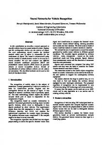
examples. Therefore, eight tests are done. The result for each data set is the average of the eight tests associated with the set. A spiral data set is a union of K subsets, s0 ; 1 1 1 ; sK 01 ; with the data in subset sk ; 0  k  K 0 1; belonging to class k: Each subset sk consists of the following two-attribute points:

sk :

x =  cos  + 2k K 2 k y =  sin  + K

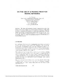
Fig. 7. Classification regions for the spiral data set of three classes.

where

 = ;  = 0:8;

0:25    4:

Fig. 6 shows the data set with three classes. We ran four spiral data sets with 3–6 classes (i.e., K = 3; 4; 5; 6), respectively. Each class contains 31 points. A comparison between our method and the two-class-based method is shown in Table I. The column “No of Attr” indicates the number of attributes associated with each example. The column “No of Classes” shows the number of classes in the underlying data set. The column “No of Examples” indicates the number of examples used for the test, which is the sum of training examples and test examples. The column “No of Neurons” shows the total number of hidden nodes in each obtained network. The column “No of Conn” indicates the total number of connections between neurons in an obtained network. Finally, the column “Rgn Rate” indicates the rate of correct classification of test examples. Note that each network obtained 100% correctly separates the training examples. Apparently, the total number of neurons is greatly reduced by our method. Fig. 7 shows the classification regions obtained by our method for the data set of three classes. As we noted earlier, spiral data sets are extremely hard. The failure in training backpropagation networks was reported in [13]. Although the trained networks can 100% correctly recognize training examples, their ability of recognizing unknown examples is still low. However, our method gets higher recognition rates than the two-class-based method. The two-class-based method replaces the inter-relationship among classes with a set of binary relationships. The examples for training are always made into two classes: positive and negative. The distinction among the examples in the negative class is ignored. We keep such inter-relationship among classes when training a neural network. So it is not surprised that our method can recognize better than the two-class-based method. However, our method takes more time in the training process than Cios and Liu’s method. Finding hyperplanes in a two-class search space is easier than in a multiclass

TABLE II COMPLEXITY FOR SPIRAL DATA

search space. We have noticed that our method spent about three and five times longer in training for the 4-class and 6-class spiral data sets, respectively. Note that classification regions for spiral data can be improved using nonlinear activation functions; the decision boundaries are smoother and the number of fragments is reduced [14]. Clearly, the complexity, i.e., the number of layers and the number of nodes in each layer, of an obtained network depends on the problem under investigation. In general, each hyper-region of the second hidden layer requires one node for each side in the first hidden layer. At the next layer, a node is needed to carry out an AND operation on that collection of hyper-regions, and so on until all the hyper-regions of each class can be linearly separated from those of the other classes by an output node. Let n1 2 n2 2 1 1 1 2 nk denote that layer 1 contains n1 nodes, layer 2 contains n2 nodes, 1 1 1 ; and layer k contains nk nodes. Table II lists the complexity of each network for spiral data set. Note that input and output nodes are not shown. We ran four data sets from [22]. Iris Plants and Thyroid Gland are three-class data sets. The three classes for Iris Plants are Setosa, Versicolor, and Virginica, and the classes for Thyroid Gland are “normal,” “hyper,” and “hypo.” Glass Identification is a seven-class data set with nine attributes. However, there is no data points for class

452

IEEE TRANSACTIONS ON SYSTEMS, MAN, AND CYBERNETICS—PART B: CYBERNETICS, VOL. 29, NO. 3, JUNE 1999

TABLE III COMPARISON WITH FOUR PRACTICAL DATA SETS

our method and the two-class-based method with these derived data sets is shown in Table IV. Apparently, our method gets much higher recognition rates than Cios and Liu’s method. However, we get more connections. Also, our method runs slower in training, e.g., about two and five times slower for the four- and six-class cases, respectively. VI. CONCLUSION

TABLE IV COMPARISON WITH THREE DERIVED DATA SETS FOR LETTER RECOGNITION (WITH 16 ATTRIBUTES)

seven. So we treat it as a six-class data set. Iris Plants contains 50 data points for each class. For Thyroid Gland, we have 150 examples for “normal,” 35 examples for “hyper,” and 30 examples for “hypo.” For Glass Identification, there are 70, 76, 17, 13, nine, and 29 examples, respectively, for its classes, making 214 examples in total. The 4-class Abalone data set is a subset of the original Abalone data set which predicts the age of abalone from eight physical measurements. Each class in 4-class Abalone contains about in 4-class Abalone contains about 62 examples. The comparison between our method and the two-class-based method with these data sets is shown in Table III. The column “Name of Data Set” shows the name of the data set associated with each example, and the other columns have the same meanings as those in Table I. Classification for the first two data sets is easy, resulting in a small number of neurons in each network. However, our method produces smaller networks. The recognition rates of both methods are equal. Both methods spend about the same time in training a network. For Glass Identification, our method results in fewer neurons and a higher recognition rate, but the number of connections is larger. As mentioned in the previous section, each node in a hidden layer is connected by all the nodes of lower layers. The number of connections increases fast if a network has many layers. Our method may result in a network with more layers than any subnetwork obtained by Cios and Liu’s method. So it is possible that our networks have more connections even though they have fewer hidden nodes. For 4-class Abalone, our method gets a smaller network as well as a higher recognition rate than the two-class-based method. Finally, we present the results with a data set concerning letter image recognition, also obtained from UCI Repository of Machine Learning Databases. The original data set has 26 classes, with 16 attributes. We selected four, five, and six classes from the original set and made three derived data sets. The selection criterion was to make the number of examples for each class about equal in respective derived data set. For the four-class set, we have 92 examples for class “C,” 96 examples for class “G,” 94 examples for class “O,” and 97 examples for class “Q,” making 379 examples in total. For the fiveclass set, we have 472 examples in total for classes “K,” “M,” “N,” “S,” and “Z.” For the 6-class set, we have 572 examples in total for classes “B,” “E,” “F,” “H,” “R,” and “P.” The comparison between

A neural network for supervised multiclass discretization may be obtained by combining subnetworks each of which is for one class and is generated by the entropy-based method proposed by Cios and Liu [5]. Since the inter-relationship among classes is reduced to a set of binary relationships and entropy is considered locally in each independent two-class subnetwork, hidden nodes cannot be shared among different classes and the recognition rate is low. We keep the inter-relationship among classes when training a neural network. Entropy measure is considered in a global sense, not locally in each independent subnetwork. Consequently, our method allows hidden nodes and layers to be shared among classes, and presents higher recognition rates than the two-class-based method. We have defined two entropy measures. One is for generating as few hidden nodes as possible, and the other one is for generating output nodes each of which separates one class from the other classes. We have developed delta rules to guide the search for optimal hyperplanes. To help delta rules escape from local minima, a simulated annealing technique called the Cauchy machine is used. ACKNOWLEDGMENT Constructive comments from the anonymous referees are appreciated. REFERENCES [1] D. H. Ackley, G. E. Hinton, and T. J. Sejnowski, “A learning algorithm for Boltzmann machines,” in Neurocomputing, J. A. Anderson and E. Rosenfeld, Eds. Cambridge, MA: MIT Press, 1985, pp. 638–650. [2] M. Bichsel and P. Seitz, “Minimum class entropy: A maximum information approach to layered networks,” Neural Networks, vol. 2, pp. 133–141, 1989. [3] K. Binder, Monte Carlo Methods in Statistical Physics. New York: Springer, 1978. [4] L. Breiman, J. H. Friedman, R. A. Olshen, and C. J. Stone, Classification and Regression Trees. Belmont, CA: Wadsworth, 1984. [5] K. J. Cios and N. Liu, “A machine learning method for generation of a neural network architecture: A continuous ID3 algorithm,” IEEE Trans. Neural Networks, vol. 3, pp. 280–290, 1992. [6] S. E. Fahlman and C. Lebiere, “The cascade-correlation learning architecture,” Tech. Rep. CMU-CS-90-100, School Comput. Sci., Carnegie Mellon Univ., Pittsburgh, PA, 1990. [7] U. M. Fayyad and K. B. Irani, “On the handling of continuous-valued attributes in decision tree generation,” Mach. Learn., vol. 8, pp. 87–102, 1992. [8] R. M. Goodman, C. M. Higgins, and J. W. Miller, “Rule-based neural network for classification and probability estimation,” Neural Computat., vol. 4, pp. 781–804, 1992. [9] W. Hastings, “Monte Carlo sampling methods using Markov chains and their application,” Biometrika, vol. 57, pp. 97–109, 1970. [10] S. Y. Kung and J. N. Hwang, “An algebraic projection analysis for optimal hidden units size and learning rate in backpropagation learning,” in Proc. IEEE Int. Conf. Neural Networks, San Diego, CA, July 1988, pp. 363–370. [11] S. Y. Kung, Digital Neural Networks. Englewood Cliffs, NJ: PrenticeHall, 1993. [12] P. J. M. Laarhoven and E. H. L. Aarts. Simulated Annealing: Theory and Applications. New York: Reidel, 1987. [13] K. Lang and M. J. Witbrock, “Learning to tell two spirals apart,” in Proc. Connectionist Models Summer School, 1988, pp. 52–59. [14] S.-J. Lee and M.-T. Jone, “An extended procedure of constructing neural networks for supervised dichotomy,” IEEE Trans. Syst., Man, Cybern. B, vol. 26, pp. 660–665, Aug. 1996.

IEEE TRANSACTIONS ON SYSTEMS, MAN, AND CYBERNETICS—PART B: CYBERNETICS, VOL. 29, NO. 3, JUNE 1999

[15] J. L. McClelland and D. E. Rumehart, Parallel Distributed Processing (Two Volumes). Cambridge, MA: MIT Press, 1986. [16] J. P. Nadal, “New algorithms for feedforward networks,” in Neural Networks and SPIN Classes, Theumann and Koberle, Eds. Singapore: World Scientific, 1989, pp. 80–88. [17] N. J. Nilsson, Learning Machines: Foundations of Trainable Pattern Classifying Systems. New York: McGraw-Hill, 1965. [18] Y. H. Pao. Adaptive Pattern Recognition and Neural Networks. Reading, MA: Addison-Wesley, 1989. [19] J. R. Quinlan, “Induction of decision trees,” Mach. Learn., vol. 1, no. 1, pp. 81–106, 1986. [20] H. Szu and R. Hartley, “Fast simulated annealing,” Phys. Lett. A, vol. 122, pp. 157–162, 1987. [21] L. Wessels, E. Barnard, and E. ven Rooyen, “The physical correlates of local minima,” in Proc. Int. Neural Networks Conf., Paris, France, July 1990, pp. 985–992. [22] P. M. Murphy and D. W. Aha “UCI repository of machine learning databases,” Dept. Inform. Comput. Sci., Univ. Calif., Irvine.

Robust Neural Adaptive Stabilization of Unknown Systems with Measurement Noise George A. Rovithakis

Abstract—In this paper, we consider the problem of adaptive stabilizing unknown nonlinear systems whose state is contaminated with external disturbances that act additively. A uniform ultimate boundedness property for the actual system state is guaranteed, as well as boundedness of all other signals in the closed loop. It is worth mentioning that the above properties are satisfied without the need of knowing a bound on the “optimal” weights, providing in this way higher degrees of autonomy to the control system. Thus, the present work can be seen as a first approach toward the development of practically autonomous systems. Index Terms—Measurement noise, neural networks, nonlinear systems, robust adaptive control.

I. INTRODUCTION Stabilization, is a key problem in control systems analysis and design, since it is the first and most important property that has to be achieved in order for a system to be well functioning. It consists of designing an appropriate feedback law that renders the system stable, (insensitive), due to external disturbances, as well as modeling error effects, caused by imperfect modeling of the actual plant. In the linear systems case, the problem has found satisfactory solution even if the real system is contaminated with noise, (sensor noise, actuator noise), and/or there exist uncertainty in system parameters or dynamics. Unfortunately, this is not the case when nonlinear systems are considered. Existing results are constrained to certain system classes and suffer from strong restrictions imposed by the currently available schemes. More analytically, the uncertainty constraint schemes [1]–[4] assume restrictive matching assumptions, while the nonlinearity constraint schemes [5]–[9] impose restrictions, (Lipschitz conditions), on the type of nonlinearities. The above nonlinear adaptive stabilization techniques are based on the complete Manuscript received March 16, 1996; revised October 22, 1997. This paper was recommended by Associate Editor P. Borne. The author is with the Department of Electronic and Computer Engineering, Technical University of Crete, 73100 Chania, Crete, Greece. Publisher Item Identifier S 1083-4419(99)00906-1.

453

knowledge of system nonlinearities and the existence of no modeling error term. Recently, works have appeared toward the direction of extending the above mentioned nonlinear adaptive control schemes, to cover the presence of modeling errors and disturbances, [10]–[12]. A generalization of adaptive stabilizers to include the case where the actual nonlinearities are unknown, using neural networks, have also appeared recently [13]–[18]. The key idea in the above works is to substitute the unknown nonlinearities by neural network structures, exploiting in this way their proven approximation properties [23]–[27]. Thus the problem is transformed into a robust nonlinear adaptive control problem. One major issue left open in [13]–[18] is how to use neural networks to adaptively stabilize unknown nonlinear systems when the output is contaminated with noise which acts additively. The problem has a strong theoretical as well as practical importance since sensor noise is a common source of malfunction in real world applications. In this paper a first solution is provided. By making use of Lyapunov stability arguments, control and update laws are developed to guarantee a uniform ultimate boundedness property for the actual system state, plus boundedness of all other signals in the closed loop. Another important aspect of the proposed control scheme, is that knowledge of a bound on the optimal1 weights is not required. However, the opposite is a prerequisite in all works that involve neural networks up to now. Hence, the proposed stabilizer can effectively be used in uncertain and rapidly changing environments, where such regions are difficult or even impossible to be given a priori, providing in this way higher degrees of autonomy to the actual system. However, the price paid for such a property is that the actual system state cannot converge asymptotically, (or arbitrarily close), to the equilibrium x = 0: In fact it can be proven that it converges to a ball whose radius possess a minimum, which we cannot exceed. The above property actually outlines the qualitative behavior of the proposed stabilizer. The paper is organized as follows: in Section II the problem is stated. Section III gives the mathematical details as well as the main result of the work. Simulation results performed on a real system are presented in Section IV. Finally, Section V concludes the paper. A. Notation The following notations and definitions will extensively be used throughout the paper. I denotes the identity matrix. j 1 j denotes the usual Euclidean norm of a vector. In case where y is a scalar, jyj denotes its absolute value. If A is a matrix, then kAk denotes the Frobenius matrix norm [19], defined as kAk2 = 6ij jaij j2 = trfAT Ag where trf1g denotes the trace of a matrix. Recall also the following definitions: Definition 1.1: Given a solution z (1): [t0 ; t1 ] !