Constructing prediction intervals for monthly

ISSH - Stochastic Hydraulics 2005 - 23 and 24 May 2005 - Nijmegen - The Netherlands

Constructing prediction intervals for monthly streamflow forecasts Wen Wang1, 2 , Pieter H.A.J.M. Van Gelder2, J. K. Vrijling2 [1] Faculty of Water Resources and Environment, Hohai University, Nanjing, 210098, China [2] Faculty of Civil Engineering & Geosciences, Section of Hydraulic Engineering, Delft University of Technology. 2600 GA Delft, Netherlands

ABSTRACT: Interval forecasts are important to supplement point forecasts, especially for medium- and long-range forecasting, so as to define the predictive uncertainty. In this study, the empirical approach and bootstrap approach based on the residuals from AR models are applied to construct prediction interval (PI) for monthly streamflow forecasts. The results show that both empirical approach and bootstrap method work reasonably well, and empirical approach gives results comparable to or even better than bootstrap method. Because of the simplicity and calculation-effectiveness, empirical method is preferable to the bootstrap method. 1 INTRODUCTION Forecasts are often expressed as single numbers, called point forecasts. The vast majority of research in hydrologic forecasting, as well as most operational hydrological forecasting systems, centers around producing and evaluating point forecasts. Point forecasts are of course of first-order importance. However, point forecasts gives no information about predictive uncertainty which is of vital importance in planning and decision making. Interval forecasts are important to supplement point forecasts, especially for medium- and long-range forecasting. Interval forecasts usually consists of an upper and a lower limit (prediction interval, PI) between which the future value is expected to lie with a prescribed probability, or a probability distribution function of the predictand (the variate being forecasted). Hirsch (1981) stated that the presentation of a single “most likely” hydrograph is of no value in long-range hydrologic forecasting. A variety of approaches to computing PIs are available (e.g., Chatfield, 1993). However, no generally accepted method exists for calculating PIs except for forecasts calculated conditional on a fitted probability model, for which the variance of forecast errors can be readily evaluated (Chatfield, 2001). In the hydrologic community, many efforts have been made on evaluating the forecast uncertainty, which is essentially equivalent to constructing PIs, in hydrologic modelling in the last two decades or so (e.g., Kitanidis & Bras, 1980; Beven & Binley, 1992; Freer et al., 1996; Kuczera & Parent, 1998; Krzysztofowicz, 1999). Four types of approaches have been proposed and used for hydrologic forecasting so far.

(1) Develop a stochastic model of streamflow based on the historic record. Initialize the model’s state variables to present conditions and use a random number generator to produce multiple (equally likely) traces from this one initial condition. The simplest model is the autoregressive (AR) model. Hirsh (1981) developed this method, where a periodic ARMA model is used to describe monthly streamflow processes. This method relies on assumptions of normality and independence of the error terms of the PARMA model. (2) Produces multiple estimates of a streamflow variable with a deterministic hydrologic model based on current basin conditions and past meteorological observations (rain, snow, temperature, humidity, wind). This method is called Extended Streamflow Prediction (ESP) (Day, 1985). It produces probabilistic forecasts by doing statistical analysis of ensemble traces. The ensemble traces are simulated by inputting historical meteorological time series, which are assumed to represent possible realizations in the future, into the hydrological model, using the current watershed conditions as the initial conditions. Then, the cumulative distribution function of the ensemble traces is estimated by weighting each trace, using the method proposed by Smith et al. (1992). Finally, the probability distribution forecasts are produced for future runoff volume in terms of nonexceedance probability by statistical analysis of the ensemble traces. The ESP forecast system has been applied as part of the National Weather Service (NWS) River Forecast System (NWSRFS) in the United States. NWS has ex-

tended the original idea to facilitate incorporation of climate outlooks into the ESP (Perica, 1998). The NWS ESP program produces ensemble traces by inputting historical meteorological events adjusted with meteorological and climatological forecasts, and deterministic precipitation forecasts. ESP approach is also taken by European Flood Forecasting System (EFFS) for making up to 10 days ahead probabilistic flood forecast (De Roo et al., 2003), but medium-range ensemble weather forecasts, instead of historical weather data, are used to generate ensemble traces. (3) Estimate the predictive uncertainty associated with hydrologic models based on Monte Carlo simulation. This method is called GLUE (Generalised Likelihood Uncertainty Estimation) proposed by Beven & Binley (1992). By specifying the sampling ranges for each parameter to be considered, as well as a formal definition of the likelihood measure to be used and the criteria for acceptance or rejection of the models, a sample of parameter sets are selected by Monte Carlo simulation, using uniform random sampling across the specified parameter range. The predictions of the Monte Carlo realisations are then weighted by the likelihood measures to formulate a cumulative distribution of predictions from which uncertainty quantiles can be calculated. A major limitation of the GLUE methodology is the dependence on Monte Carlo simulation, which requires considerable computing resources. For complex models requiring a great deal of computer time for a single run, it will not be possible to fully explore high order parameter response surfaces. (4) Bayesian theory based probabilistic forecast method is recently proposed by Krzysztofowicz (1999). The basic idea of Bayesian prediction is to blend together prior and posterior information using Bayes theorem. In the BFS, the total uncertainty is decomposed into two sources: (1) input uncertainty associated with random inputs (mainly, precipitation) and (2) hydrologic uncertainty arising from all sources beyond those classified as random inputs, including model, parameter, estimation, and measurement erros. BFS offers a theoretically derived structure to quantify the input uncertainty and hydrologic uncertainty and then integrate all those uncertainties into a predictive (Bayes) distribution. Among the four approaches mentioned above, only the first one is suitable for univariate stochastic time series model, whereas the other three are based on more complicated models that are datademanding and usually assumed to be true. However, the approach (1) relies on the assumption of normality, which is not often justified in actual applications. Therefore, In this study, we will construct

PI of monthly streamflow forecasts based on the residuals from univariate ARMA models. We will apply residual based methods that are independent of any assumption for constructing PIs for monthly streamflow forecasting. 2 METHODOLOGY Seasonal time series (i.e., most streamflow processes) are commonly modelled with three types of time series models (Hipel & McLeod, 1994): (1) seasonal autoregressive integrated moving average (SARIMA) models; (2) deseasonalized ARMA models; and (3) periodic ARMA models. In this study, the second modeling strategy, i.e., deseasonalized ARMA models, is adopted. Although theoretical formulae are available for computing PIs for ARMA-type time-series model (Box & Jenkins, 1976), it is well-known that streamflow processes often have heavy tails (e.g., Anderson & Meerschaert, 1998), therefore, theoretical formulae which assume normality are not applicable. In contrast with theoretical method, residual based PI estimation methods do not require any distributional assumptions. Two methods will be used in this study to estimate PIs based on residuals, i.e., empirical method and bootstrap-based method. Empirical method constructs PIs relying on the properties of the observed distribution of residuals (rather than on an assumption that the model is true). Bootstrap-based method samples from the empirical distribution of the residuals from fitted models to construct a sequence of possible future values, and evaluates PIs at different horizons by simply finding the interval within which the required percentage of resampled future values lies. 2.1 Empirical PI construction Let {xt} be a sequence of n observed streamflow series. The empirical PI estimation for k-step ahead prediction proceeds as follows: Step 1. Logarithmize the streamflow series, and then deseasonalize the logarithmized series by subtracting the monthly mean values and dividing by the monthly standard deviations of the logarithmized series. Step 2. Fit AR(p) model to the transformed series, in the form of φ ( B ) xt = ε t , where φ(B) represents the ordinary autoregressive components. Compute the kstep ahead fitted error (residuals): p

ε t + k = xt + k − ∑ φ j xt + k − j , t = p + 1,..., n − k . j =1

(1)

ISSH - Stochastic Hydraulics 2005 - 23 and 24 May 2005 - Nijmegen - The Netherlands

Notice that, when k-j ≥ 1, calculated value (with p

xt = ∑ φ j xt − j ), instead of the observed value, will j =1

be used for xt+k-j in the Equation (1). Step 3. Define the empirical distribution function Fε,k of the residuals εt+k: n 1 Fε ,k ( x) = (2) 1{ε ≤ x} ∑ n − p t = p +1 t +k Step 4. Obtain the upper bound of k-step ahead future value by expression p

xnU+ k = ∑ φ j xn + k − j + ε nU+ k ,

(3)

j =1

and the lower bound by p

xnL+ k = ∑ φ j xn + k − j + ε nL+ k

(4)

j =1

where ε nU+ k and ε nL+ k are the upper and lower p/2-th empirical quantile drawn from Fε,k according to the nominal coverage level (1-p). Notice that, as in step 2, when k-j ≥ 1, calculated value will be used for xt+k-j in the Equation (3) as well as in the Equation (4). Step 5. Inversely transform the upper and lower bounds to their original scale. 2.2 Bootstrap PI construction Bootstrap method is a distribution-free, but computationally intensive approach. There are several bootstrap alternatives in the literature to construct prediction intervals for AR processes (e.g., Stine, 1987; Thombs & Schucany, 1990). In this study, we use the method recently proposed by Pascual et al. (2004), which has the advantage over other bootstrap methods previously proposed for autoregressive integrated processes that variability due to parameter estimation can be incorporated into prediction intervals without requiring the backward representation of the process. Consequently, the procedure is very flexible and can be extended to processes even if their backward representation is not available. Furthermore, its implementation is very simple. The steps for obtaining bootstrap prediction intervals for monthly streamflow processes are as follows: Step 1. The same as Step 1 in Section 2.1. Step 2. Fit AR(p) model to the transformed series, in the form of φ ( B ) xt = ε t . Compute the one-step fitted error (residuals) εt as in Eq. (1), where k=1. Step 3. Let Fε be the empirical distribution function of the centered and rescaled residuals by the factor [(n-p)/(n-2p)] 0.5. Step 4. From a set of p initial values, generate a bootstrap series from p xt* = ∑ φ j xt*− j + ε t* (5) * j =1 where εt are sampled randomly from Fε.

Step 5. Use the generated bootstrap series to reestimate the original model, and obtain one bootstrap draw of the autoregressive coefficients φ *= (φ1*, φ2*,…, φp*). Step 6. Generate a bootstrap future value through the recursion of the AR model with the bootstrap parameters * n+k

x

p

= ∑ φ *j xn*+ k − j + ε n*+ k

(6)

j =1

with εt* a random draw from Fε; xn+h*= xn+h for h ≤ 0. Step 7. Repeat the last three steps B times (e.g., 1000 or 2000) and then go to step 8. Step 8. The endpoints of the prediction interval are given by quantiles of GB*, the bootstrap distribution function of xn+k*. Step 9. Inversely transform the upper and lower bounds to their original scale. 3 DATA USED Monthly streamflow series of four rivers, i.e., the Yellow River in China, the Rhine River in Europe, the Umpqua River and the Ocmulgee River in the United States, are analyzed in this study. The first streamflow process is the streamflow of the upper Yellow River at Tangnaihai. The gauging station Tangnaihai has a 133,650 km2 drainage area in the northeastern Tibet Plateau. Most of the watershed is 3000 ~ 6000 meters above sea level. Snowmelt water composes about 5% of total runoff. Because the watershed is partly permanently snow-covered and sparsely populated, without any large-scale hydraulic works, the streamflow process is fairly pristine.

The second one is the streamflow of the Rhine River at Lobith, the Netherlands. The gauging station Lobith is located at the lower reaches of the Rhine, near German-Dutch border, with a drainage area is about 160,800 km2. Due to favorable distribution of precipitation over the catchment area, the Rhine has a rather equal discharge. The data are provided by the Global Runoff Data Centre (GRDC) in Germany (http://grdc.bafg.de/). The third one is the streamflow of the upper Ocumlgee River at Macon, Georgia in the United States. The station Macon has a drainage area of 5,799 km2. The headwaters of the Ocmulgee River begin in the highly urbanized Atlanta metropolitan area, and downstream its watershed is dominated by agriculture and forested areas. The fourth one is the streamflow of the Umpqua River near Elkton, Oregon also in the United States. The drainage area is 9,535 km2. Regulation by powerplants on North Umpqua River ordinarily does not affect discharge at this station. There are diversions for irrigation upstream from the station. The daily discharge data of both the Ocmulgee River and the Umpqua River are

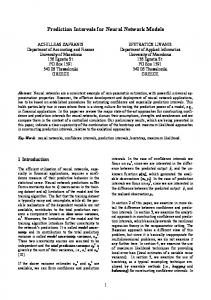
available from the USGS (United States Geological Survey) website http://water.usgs.gov/waterwatch/. Monthly series are obtained from daily data by taking the average of daily discharges in every month. The mean monthly discharges of these streamflow series over the year are plotted in Figure 1.

siduals are defined according to fitted error from the AR models fitted to the first part. But in the practice, all the fitted residuals up to the forecast point could be used. 4.2 Construct PIs according to the overall empirical distribution function of residuals

3

Discharge(m /s)

3000 2500

Rhine

2000

Yellow

1500

Umpqua Ocmulgee

1000 500 0 0

2

4

6

8

10

12

Month

Figure 1 Average monthly discharges of four monthly streamflow processes

4 APPLICATION OF THE TWO PI CONSTRUCTION METHODS

4.1 Split the data set and fit AR models It has been analyzed that the four monthly streamflow series are basically stationary (Wang et al., 2005) although it is well known that streamflow processes exhibit seasonality in their mean values, variances and autocorrelation structures. Hence, no pre-processing (e.g., detrending or differencing) is needed. All the streamflow series are transformed with logrithmization and deseasonalization. Then we split each series into two parts, with the first part for fitting ARMA models and getting the residuals and the second part for constructing prediction intervals with the ARMA models fitted to the first part. Chernick (1999, pp 150-151) suggested that the sample size for bootstrap sampling should be larger than 30. To meet the requirement, we keep the size of first part larger than 360 (i.e., 30 years for monthly series), so that when generating bootstrap samples for each individual month, we have a sample size larger than 30. The orders of the AR models fitted to the first parts of each transformed flow series are chosen according to AIC. The details of the data size, the partition of the data set and the order of AR models for each series are listed in Table 1. Table 1 Data size, the partition of the data set and the order of AR models River Data period Part 1 Part 2 AR(p) Yellow 1956-2000 420 120 4 Rhine 1901-1996 600 552 4 Ocmulgee 1929-2001 444 432 3 Umpqua 1906-2001 600 552 5

In this study, only one-step ahead forecast is considered, and the empirical distribution function of re-

The 95% probability is commonly applied to build prediction interval. However, for a 95% probability, PIs may become so embarrassingly wide that they are of little practical use other than to indicate the high degree of future uncertainty. Granger (1996) suggests using 50%, rather than 95%, PIs because this gives intervals that are better calibrated in regard to their robustness to outliers and to departures from model assumptions. Such intervals will be narrower but imply that a future value has only a 50% chance of lying inside the interval. Therefore, Chatfield (2001) suggests using 90% or 80% prediction interval. In this study, we build the 95%, 90%, 80% and 50% PIs for one-step ahead monthly average discharge prediction with the methods described in Section 2. For the bootstrap procedure, B = 1000. To evaluate the performance of PI construction methods, the following measures are used: the actual PI coverage, the average PI length, the proportions of observations lying out to the left and to the right of the interval. A good PI construction method should have a coverage close to the nominal coverage, a small interval length, and balanced proportions of observations below and above the interval. Table 2 reports the results for the four monthly streamflow processes, comparing empirical PIs with bootstrap-based PIs. It is shown that both methods give reasonable performance in terms of interval coverage, and there is no significant bias of the interval, namely, the numbers of observed values falling to the left and to the right of the interval are mostly close. In terms of the interval length, empirical method outperform the bootstrap method because empirical method has generally shorter interval length. Since the streamflow processes exhibit strong seasonality as shown in Figure 1, to inspect possible impacts of the presence of seasonality on the performance of empirical method and bootstrap method, we check the PIs month by month. Table 3 lists PI construction results for these flow series with nominal coverage of 80% month by month (to save space, results for other three nominal coverage levels are not listed here).

ISSH - Stochastic Hydraulics 2005 - 23 and 24 May 2005 - Nijmegen - The Netherlands

Table 2 Prediction intervals for monthly flow series Nominal Yellow Rhine Ocmulgee Umpqua Measure Cov. Emp. Boot. Emp. Boot. Emp. Boot. Emp. Boot. Cov. 0.925 0.925 0.964 0.94 0.938 0.91 0.964 0.944 Above Cov. 0.033 0.033 0.016 0.034 0.016 0.021 0.016 0.027 95% Below Cov. 0.042 0.042 0.02 0.025 0.046 0.069 0.02 0.029 Average Len. 623 704 2828 2798 171 190 437 430 Cov. 0.875 0.892 0.879 0.888 0.882 0.856 0.908 0.902 Above Cov. 0.05 0.042 0.067 0.054 0.046 0.042 0.027 0.049 90% Below Cov. 0.075 0.067 0.054 0.058 0.072 0.102 0.065 0.049 AverageLen. 473 551 1996 2266 118 134 350 355 Cov. 0.742 0.742 0.784 0.772 0.762 0.736 0.806 0.821 Above Cov. 0.117 0.092 0.12 0.123 0.095 0.118 0.087 0.092 80% Below Cov. 0.142 0.167 0.096 0.105 0.144 0.146 0.107 0.087 Average Len. 346 438 1500 1582 89 91 247 276 Cov. 0.5 0.5 0.527 0.518 0.491 0.451 0.504 0.489 Above Cov. 0.2 0.192 0.252 0.248 0.255 0.269 0.268 0.281 50% Below Cov. 0.3 0.308 0.221 0.234 0.255 0.28 0.228 0.23 Average Len. 171 225 851 867 43 47 110 124 Note: Cov. - coverage; Len. - length; Emp. - empirical method; Boot. - bootstrap method. Table 3 Month by month PI coverages for monthly flow with nominal coverage of 80% Yellow Rhine Ocmulgee Umpqua Month Emp. Boot. Emp. Boot. Emp. Boot. Emp. Boot. 1 0.900 0.700 0.717 0.783 0.833 0.944 0.717 0.739 2 0.900 0.700 0.696 0.804 0.722 0.722 0.652 0.739 3 1.000 0.500 0.696 0.739 0.722 0.722 0.739 0.761 4 0.200 0.400 0.739 0.761 0.667 0.639 0.761 0.891 5 0.800 0.800 0.848 0.804 0.722 0.694 0.783 0.870 6 0.500 0.500 0.826 0.717 0.861 0.889 0.891 0.848 7 0.500 0.500 0.761 0.739 0.722 0.528 0.957 0.783 8 0.500 0.900 0.913 0.848 0.750 0.500 0.957 0.870 9 0.600 1.000 0.891 0.848 0.722 0.750 0.913 0.870 10 1.000 1.000 0.804 0.739 0.806 0.778 0.848 0.891 11 1.000 0.900 0.761 0.717 0.861 0.833 0.696 0.826 12 1.000 1.000 0.761 0.761 0.750 0.833 0.761 0.761

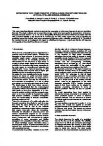
quantile for the nominal coverage (1-p) is too large for low-flow months, and too small for high flow months, which causes the systematic bias of PI coverages shown in Table 3. 1 Yellow Rhine Ocmulgee Umpqua

0.8 SD

From Table 3, we find that there is a systematic bias that for low-flow months the coverage of PIs is larger than the nominal coverage, whereas for high-flow months the coverage of PIs is smaller than the nominal coverage, especially for the Yellow River and the Umpqua River. That indicates that for low-flow months the PIs are overestimated, and for high-flow months the PIs are under-estimated. We examine the standard deviation of the residuals of the months over the year, plotted in Figure 2. It is shown that for the Yellow River and Umpqua River, there is obvious seasonal variation in standard deviation of the residuals. Comparing Figure 1 and Figure 2, we can find that there is a general tendency that the months with high flow also have high residual standard deviation. Therefore, when we use the overall empirical distribution function to construct the PIs, the coverage between the upper and lower p/2-th empirical

0.6 0.4 0.2 0

2

4

6 Month

8

10

12

Figure 2 Seasonal variation in standard deviation (SD) of the residuals

Table 4 PIs considering the seasonal variation in variance of the residuals Yellow Rhine Ocmulgee Nominal Measure Cov. Emp. Boot. Emp. Boot. Emp. Boot. Cov. 0.917 0.933 0.953 0.937 0.905 0.905 Above Cov. 0.042 0.025 0.036 0.033 0.039 0.023 95% Below Cov. 0.042 0.042 0.011 0.031 0.056 0.072 Average Len. 597 710 2768 2807 147 189 Cov. 0.875 0.892 0.899 0.886 0.824 0.859 Above Cov. 0.067 0.042 0.058 0.058 0.079 0.042 90% Below Cov. 0.058 0.067 0.043 0.056 0.097 0.100 Average Len. 513 553 2316 2276 110 132

Umpqua Emp. Boot. 0.957 0.944 0.027 0.025 0.016 0.031 424 432 0.911 0.911 0.049 0.043 0.040 0.045 357 355

Table 5 Month by month PI coverages for monthly flow with nominal coverage of 80% (considering the seasonal variation in variance of the residuals) Yellow Rhine Ocmulgee Umpqua Month Emp. Boot. Emp. Boot. Emp. Boot. Emp. Boot. 1 0.700 0.700 0.783 0.783 0.944 0.944 0.739 0.739 2 0.700 0.700 0.739 0.826 0.722 0.750 0.739 0.739 3 0.800 0.600 0.783 0.804 0.694 0.722 0.783 0.783 4 0.500 0.400 0.783 0.761 0.611 0.667 0.848 0.870 5 0.800 0.800 0.804 0.804 0.694 0.694 0.870 0.870 6 0.400 0.500 0.717 0.717 0.833 0.917 0.848 0.848 7 0.600 0.500 0.739 0.761 0.528 0.528 0.783 0.783 8 0.900 0.900 0.848 0.848 0.500 0.500 0.761 0.783 9 1.000 1.000 0.826 0.826 0.694 0.722 0.848 0.848 10 1.000 1.000 0.717 0.717 0.778 0.833 0.870 0.891 11 0.900 0.900 0.717 0.717 0.667 0.833 0.804 0.826 12 1.000 1.000 0.761 0.783 0.778 0.833 0.761 0.739

4.3 Construct PIs according to the seasonal empirical distribution function of residuals To take the season-dependant variance of residuals into account, we define the seasonal empirical distribution function Fε(m) for the residuals of each month m. Then choose the upper and lower p/2-th empirical quantile for the nominal coverage (1-p) from Fε(m) for empirical PI construction method, and generate bootstrapping samples from Fε(m) for the bootstrap method, so that we construct the PIs considering the seasonal variation in variance of the residuals. Table 4 lists the results for the streamflow processes with the seasonal variation in variance considered. Comparing with Table 2, we observe that no significant improvement are achieved in terms of PI coverages after considering the seasonal variation in variance. The values of coverage length are even bigger than those without considering seasonal variation in variance. However, when we examine the PIs month by month, as shown in Table 5 for nominal coverage 80%, it is clear that the systematic bias shown in Table 3 disappears, and maximum errors between the nominal coverage and actual coverage are reduced, especially

for the empirical method. For example, for the Umpqua River, the range of the difference between the nominal coverage and actual coverage with the empirical method is –0.148 (= 0.652 – 0.8) to 0.157 (=0.957 – 0.8) before considering seasonal standard deviation in residuals, and shrinks to –0.039 (= 0.761- 0.8) to 0.07 (=0.870 – 0.8) after considering seasonal standard deviation. Therefore, by considering the seasonal variation in variance of the residuals, more accurate PI construction is obtained. Figure 3 plots the observed discharges during 1991 to 2000 of the Yellow River and their upper and lower prediction bounds for 80% nominal coverage constructed using the empirical method considering the seasonal empirical distribution function of residuals. At the same time, we should notice that for streamflow series, like the monthly streamflow of the Ocmulgee, which exhibits no significant seasonal variation in variance in the residuals, to construct PI according to the seasonal empirical distribution function of residuals may deteriorate the PI construction results, because the seasonal empirical distribution function of residuals are defined with a much smaller sample size (for monthly streamflow series, the size is reduced to 1/12), which may cause error for PI construction.

ISSH - Stochastic Hydraulics 2005 - 23 and 24 May 2005 - Nijmegen - The Netherlands 4000 Observed 80% lower bound 80% upper bound

Dishcarge (m3/s)

3500 3000 2500 2000 1500 1000 500 0 1

13

25

37

49

61 Month

73

85

97

109

Figure 3 Observed monthly discharges (1991-2000) of the Yellow River and their 80% upper and lower prediction bounds. Beven, K. J., & Binley, A. 1992. The future of distributed models: Model calibration and uncertainty prediction, Hydrol. Processes, 6, 279– 298. Box, G.E.P., & Jenkins, G.M. 1976. Time series Analysis: Forecasting and Control (2nd edition), Holden-Day, San Francisco Chatfield, C. 1993. Calculating interval forecasts (with discussion), Journal of Business and Economic Statistics, 11, 121-144. Chatfield, C. 2001. Prediction intervals for time series. in Principles of Forecasting: A Handbook for Practitioners and Researchers, Armstrong, J. S. (ed.), Norwall, MA: Kluwer Academic Publishers, 475-494. Chernick, M.R. 1999. Bootstrap methods: A Practitioner’s Guide. John Wiley & Sons, New York. Christoffersen, P.F. 1998. Evaluating interval forecasts, International Economic Review, 39(4), 841-862 Day, G.N. 1985. Extended streamflow forecasting using NWSRFS. J. Water Resour. Plan. Manage., 111(2): 157170 De Roo APJ, Bartholmes J, Bates PD, Beven K et al. Development of a European Flood Forecasting System. Journal of River Basin Management, 2003, 1(1): 49-59 Freer, J., J. K. Beven, & B. Ambroise (1996), Bayesian estimation of uncertainty in runoff prediction and the value of data: An application of the GLUE approach, Water Resour. Res., 32, 2161– 2173. Hipel, K.W. & McLeod, A.I.: Time series modelling of water resources and environmental systems. Elsvier, Amsterdam, 1994 Hirsch, RM. Stochastic hydrologic model for drought management. J. Water Resour. Plan. Manage., 1981, 107(2), 303-313 Kitanidis P.K., & Bras R.L., 1980. Real-tie forecasting with a conceptual hydrologic model: 1., Analysis of uncertainty. Water Resources Research, 16(6), 1025-1033 Krzysztofowicz, R. 1999. Bayesian theory of probabilistic forecasting via deterministic hydrologic model. Water Resour. Res. 35(9), 2739-2750 Kuczera, G., & Parent E. 1998. Monte Carlo assessment of parameter uncertainty in conceptual catchment models: The Metropolis algorithm. J. Hydrol., 211, 69– 85. Pascual, L., Romo, J. & Ruiz, E. 2004. Bootstrap predictive inference for arima processes. J. Time Series Analysis, 25(4), 449-465

5 CONCLUSIONS Interval forecasts are important to supplement point forecasts, especially for medium- and long-range forecasting, so as to define the predictive uncertainty. Whatever sources of forecasting uncertainty may be, they will be reflected in residuals and therefore we can construct the prediction interval for a specific forecasting model (or method) according to the empirical distribution function of the residuals, supposing that the model (or method) is un-biased, and the hydrological process is stationary and long enough. In this study, the residual based empirical approach and bootstrap approach are applied to construct prediction interval (PI) for monthly streamflow forecasts. The results show that both empirical approach and bootstrap method work reasonably well, and empirical approach gives results comparable to or even better than bootstrap method. Because of the simplicity and calculation-effectiveness, empirical method is preferable to the bootstrap method. When there is significant seasonal variation in the variance of the residuals, to improve the PI construction, it is necessary to use seasonal empirical distribution functions which are defined by seasonal residuals rather than use overall empirical distribution functions which are defined by entire residual. The result of this study may suggest that for certain types of model, especially when non-linearities are involved (such as neural network models and the nearest neighbor method), for which theoretical formulae are not available for computing PIs, the empirical method could be a good practical choice to construct prediction interval in comparison with those more datademanding and more complicated methods, such as ESP (Day, 1985), GLUE (Beven and Binley, 1992) and Bayesian method (Krzysztofowicz, 1999).

REFERENCES Anderson P. L., & Meerschaert, M.M. 1998. Modeling river flows with heavy tails. Water Resources Research, 34(9), 2271-2280

7

Perica, S. 1998. Integration of Meteorological Forecasts/Climate Outlooks Into Extended Streamflow Prediction (ESP) System, 78th Annual AMS Meeting, Phoenix, Arizona, http://www.nws.noaa.gov/oh/hrl/papers/ams/ams986.htm Smith, J.A., Day, G.N. & Kane, M.D. 1990. Nonparametric framework for long-range streamflow forecasting. J. Water Resour. Plann. Manage. 118(1): 82-92 Stine, R.A. 1987. Estimatingpropertie s of autoregressive forecasts. J. Am. Statist. Assoc., 82, 1072–8. Thombs, L. A. & Schucany, W. R. 1990. Bootstrap prediction intervals for autoregression. J. Am. Statist. Assoc. 85, 486–92. Wang W., Vrijling J.K., Van Gelder P.H.A.J.M., & Ma J. 2005. Testing for nonlinearity of streamflow processes at different timescales, Journal of Hydrology (in press).

8