Prediction Intervals for Electricity Load Forecasting Using Neural ...

Prediction Intervals for Electricity Load Forecasting Using Neural Networks Mashud Rana, Irena Koprinska, Abbas Khosravi, and Vassilios G. Agelidis

Abstract—Most of the research in time series is concerned with point forecasting. In this paper we focus on interval forecasting and its application for electricity load prediction. We extend the LUBE method, a neural network-based method for computing prediction intervals. The extended method, called LUBEX, includes an advanced feature selector and an ensemble of neural networks. Its performance is evaluated using Australian electricity load data for one year. The results showed that LUBEX is able to generate high quality prediction intervals, using a very small number of previous lag variables and having acceptable training time requirements. The use of ensemble is shown to be critical for the accuracy of the results.

I. INTRODUCTION

W

consider the task of predicting the future electricity load (demand) from a time series of previous electricity loads. In particular, we study a time series of electricity loads measured every 30 minutes and our goal is to make predictions for the next value. Forecasting with lead times up to an hour is classified as Very Short Term Load Forecasting (VSTLF) and is a key task in the operation of electricity markets, such as the Australian national electricity market. Electricity markets balance supply and demand - the market operator forecasts the demand, suppliers make bids indicating the amount of electricity they can generate and its price, the bids are matched against the forecast and the best ones are accepted, so that the demand is met and the cost is minimized. Predicting the load accurately is essential; overpredicting increases the cost while under-predicting compromises the reliability of supply. The electricity load series data is complex. It is highly non-linear and non-stationary, with several cycles that are nested into each other, e.g. daily, weekly and yearly. In addition, it includes random components resulting from large industrial loads with irregular hours of operation, special events, holidays, extreme weather and sudden weather change. It is also noisy due to malfunctioning of data collection devices. All these factors combined together make the task of building accurate prediction models challenging. E

Manuscript received February 18, 2013. Mashud Rana and Irena Koprinska are with the School of Information Technologies, University of Sydney, Sydney, NSW 2006, Australia (e-mail: [email protected], [email protected]). Abbas Khosravi is with the Centre for Intelligent Systems Research, Deakin University, Geelong, VIC 3217, Australia (e-mail: [email protected]). Vassilios G. Agelidis is with the Australian Energy Research Institute, University of New South Wales, Sydney, NSW 2052, Australia (e-mail: [email protected]).

The most successful methods for VSTLF reported in the literature are based on Holt-Winters exponential smoothing and autoregressive integrated moving average [1-3], linear regression [4-6] and Neural Networks (NNs) [4-10]. These methods, however, focus on point forecasting, i.e. at time t the task is to predict the load value for time t+h, where h is the forecasting horizon. In this paper we focus on interval forecasting, i.e. at time t the task is to predict an interval of values for time t+h with a certain probability, called confidence level. More specifically, an interval forecast, or Prediction Interval (PI), consists of an upper and lower bound, between which the future value is expected to lie with a certain prescribed probability [11]. Predicting an interval of values with a certain probability instead of just predicting a single value gives more information about the variability of the target variable and the associated uncertainty. Hence, interval forecasts are more useful than point forecasts for risk management and quantification of the certainty of the point forecasts. They are especially suitable for applications requiring balancing of demand and supply, e.g. electricity and financial markets, stock manufacturing and inventory management [11]. A new method for constructing PIs using NNs was proposed in [12]. It is called LUBE and its main idea is to directly generate the lower and upper bounds of PIs using a feedforward NN with two outputs. LUBE uses the point forecasts for the training data and a specially designed cost function that is minimized in order to generate high quality PIs for new data. The LUBE method was compared with other NN-based methods for PI construction such as the delta [13], Baysian [14] and bootstrap methods [15]. LUBE was shown [12] to generate high quality and valid PIs, typically superior to those generated by the other methods. The comparative study also showed that LUBE was simpler to implement and more flexible as it does not make prior assumptions about the data distribution. In this paper we study the effectiveness of the LUBE method for interval forecasts for electricity load prediction. We also extend the LUBE method in two ways: 1) by incorporating feature selection and 2) by using an ensemble of LUBE NNs instead of a single NN in order to improve the reliability of the constructed PIs. The contribution of this paper can be summarized as follows: 1. We present a new method for interval forecasting, called LUBEX, an extension of the LUBE method. The extension is two-fold. Firstly, it uses an advanced feature selection method to identify a small set of

informative variables. Good feature selection is crucial for the accuracy of prediction methods. We applied a novel estimator of mutual information based on k-nearest neighbors [16]. Secondly, we construct an ensemble of LUBE NNs instead of a single NN in order to reduce the sensitivity of LUBE to the random initialization of weights, the random perturbation during training and the network architecture, and improve the stability of the results. 2. We conduct a comprehensive evaluation of the proposed LUBEX method using 30-minute data from the Australian Energy Market Operator (AEMO) [17] for one year. The results show that the proposed method is able to generate high quality interval forecasts. The rest of the paper is organized as follows. A problem statement is given in Section II. Section III presents measures for evaluating the quality of PIs. Sections IV and V describe the proposed LUBEX method. Section VI summarizes the experimental setup. Section VII presents and discusses the results. Section VIII concludes the paper.

1

. 100%, where ,

1, 0,

A required nominal confidence level 1 100% is set in advance. PIs with PICP smaller than are not reliable. PICP alone is not enough to measure the quality of a PI. The width of the interval is related to its coverage probability – wider PIs have high coverage probability and vice versa. Thus, it is possible to achieve the required minimum PICP by simply widening the interval. However, too wide intervals are useless in practice. Hence, when assessing the quality of the PI we need to consider also their width. To do this, we use the Prediction Interval Normalized Averaged Width (PINAW). It measures the average width of the PIs, for all points in the dataset, normalized by the range of the target values R: 1

II. PROBLEM STATEMENT Given is a time series containing n observations: X1, X2,…, Xn. In a standard point forecasting scenario, the goal is to forecast X n + h , the value of the series h steps ahead, using the data up to time n. In an interval prediction scenario, our goal is to forecast the PI of X n + h , i.e. its lower and upper bounds, L( X n+ h ) and U ( X n + h ) . In this paper we consider a forecasting horizon h = 1, so our task is to predict L( X n+1 ) and U ( X n+1 ) , the PI for a 1-step ahead point forecast. Given a confidence level 1 100%, a valid PI for X n +1 will satisfy the following condition: P( L( X n +1 ) ≤ X n +1 ≤ U ( X n +1 ) ) ≥ 1

, i.e. the probability that the interval will contain X n +1 will be equal or greater than the prescribed confidence level. III. EVALUATING THE QUALITY OF PIS The two most important properties of PI are coverage probability and width. A good PI will have high coverage probability and small width. While measures based on the coverage probability have been widely used to assess the quality of PIs, the width has been mostly ignored [12]. Following [12, 18], we evaluate the quality of both properties by using the three measures described below: PICP, PINAW and CWC. Given a dataset of examples, the Prediction Interval Coverage Probability (PICP) is the probability that the target value of the i-th example will fall between the upper limit and lower limit of the prediction interval , averaged over all i. PICP is calculated empirically by counting the number of target values that fall within these limits:

We also use the Coverage Width-based Criterion (CWC) [12] which combines PICP and PINAW: 1

, where 0, 1,

where and are the parameters determining the contribution of PICP and NMPIW. The two main principles of CWC are: 1) If the coverage probability is above the confidence threshold, i.e. , then CWC should depend only on the PI’s width. This is achieved by setting 0 to eliminate the exponential term. CWC becomes equal to the width PINAW and has a low value; 2) If the coverage probability is below the confidence threshold, i.e. the PIs are not reliable, CWC will have a high value, regardless of the PI’s width measured by PINAW. This is achieved by using a high value for in the exponential term and by setting 1 to consider this term. As the exponential term becomes much higher than PINAW, the influence of PINAW is lost. CWC will be high because of the high value of the exponential term. In this way, the CWC balances the usefulness of the constructed PIs (narrow width) with their correctness (acceptable coverage probability). A detailed analysis of the CWC evaluation function is given in [12]. IV. THE PROPOSED LUBEX METHOD We propose a new method for computing PI, called LUBEX, which is an extension of the LUBE method [12]. We firstly briefly describe the original LUBE method and then our proposed extension.

A. The LUBE Method The LUBE method computes PIs using feedforward NNs. It was shown to produce high quality PIs at a reasonable computational cost, outperforming other methods such as the delta [13], Bayesian [14] and bootstrap methods [15]. The main idea is to train a NN to predict the PIs. The network learns to compute PIs on a training set and is then used to predict PIs on a new set of examples. The architecture of the LUBE NN is a standard multilayer perceptron as shown in Fig.1. There are p input neurons, corresponding to the input variables of each example, and two output neurons corresponding to the lower and upper bounds of the PI for this example. There are one or more hidden layers and the number of neurons in them is set experimentally.

B. The LUBEX Method The LUBEX method is summarized in Fig. 3. We extend the LUBE method in two ways: 1) by adding a feature selection step and 2) by using an ensemble of LUBE NNs instead of a single NN.

Fig.1. The LUBE NN architecture

The LUBE NN is trained to minimize the CWC cost function. As CWC is not differentiable, the backpropagation algorithm cannot be used to do this. Instead, the LUBE NN uses the simulated annealing algorithm. The simulated annealing combines hill-climbing and random walk strategies. The latter is used to escape bad local minima. Fig. 2 gives the flow chart of the LUBE NN training. After initialization of the parameters, including the starting temperature To which is set to a high value, the starting solution (NN weights) w0 and the starting cost function CWCo, the NN is used to learn PIs for the training data. The and of the prediction interval two target values are both set to the target point forecast . The cost function CWCnew is then computed and minimized. If there is an improvement, i.e. CWCnew is less than the previous best CWC, CWCnew and wnew are accepted (hill-climbing step). Otherwise, the Metropolis criterion is used to test for acceptance (random walk step). The acceptance depends on the temperature and the badness of the new solution. The temperature is reduced as the algorithm progresses. Hence, bad solutions are more likely to be accepted at the beginning of the training. If the stopping criterion is not satisfied, a new set of weights is obtained via small perturbation and the training continues. When the training is completed, the trained NN is used to compute the PIs for the testing data. More details about the parameter setting and our implementation of the simulated annealing are presented in Section VI.

Fig. 2. The LUBE training method

1. 2. 3.

4.

Split data into training, validation and testing sets: Dtrain, Dvalid and Dtest Conduct feature selection using Dtrain and mutual information. Train an ensemble of LUBE NNs to learn the prediction intervals for Dtrain. Use Dvalid to select the architecture of the LUBE NNs. Test the performance of the ensemble on Dtest Fig. 3. The proposed LUBEX method

V. FEATURE SELECTION FOR PIS CONSTRUCTION We applied Mutual Information (MI) as a feature selection method. MI is well known feature selector in classification tasks [19, 20], but is relatively new for time series applications. It is a very useful method as it captures both linear and nonlinear dependencies. MI measures the dependence between two variables. If the two variables are independent, MI is zero; if they are dependent, MI has a positive value corresponding to the strength of the dependency. While MI has been very popular for nominal variables, its computation for continuous variables is more difficult as it requires making assumptions about the data distribution. In this work we apply the approach for MI estimation based on k-nearest neighbor distances [16]. It was shown to be efficient and more reliable than the traditional methods. The MI between two random continuous variables X and Y with dimensionality N is estimated as: ,

1

1

,

is the digamma function Γ where Γ / , k is the number of nearest neighbors (we used k=6); is the number of points with a distance to /2 and is the number of satisfying /2 is satisfying /2, where points the distance between and its k-th neighbor in the X

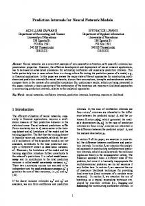
subspace and /2 is the distance between and its k-th neighbor in the Y subspace. As described in Section VI, in this paper we use halfhourly data for 12 months, called case studies (C1-C12). To conduct feature selection using MI, we first apply a 1-week sliding window consisting of 336 half-hourly lag variables, for the training data for each case study. We then compute the MI score between each of the lag variables from the sliding window and the class variable and finally rank the lag variables in decreasing order based on the MI score. 1.2 1

Merit Score by MI

0.8 0.6

C1 C4 C7 C10

C2 C5 C8 C11

C3 C6 C9 C12

0.4 0.2 0 1 18 35 52 69 86 103 120 137 154 171 188 205 222 239 256 273 290 307 324

The first extension, feature selection, is needed to reduce the data dimensionality for faster training of the prediction models and faster online use of these models, and also for improving the prediction accuracy by removing the irrelevant and redundant features. We used mutual information for feature selection as described in Section V. The second extension, using an ensemble, is necessary to improve the reliability of the generated PIs by reducing the sensitivity of the LUBE NN to the network architecture, the random initialization of the weights at the beginning and random perturbation of weights during training. LUBEX forms an ensemble of LUBE NNs using the following method. It considers NNs with one hidden layer and builds 30 NN architectures A1,..,A30 by varying the number of hidden neurons in them from 1 to 30. Using each architecture Aj, j=1,..,30, it builds an ensemble Ej of m LUBE NNs (we used m=100). The ensemble members of Ej have the same architecture Aj but are initialized to different random weights and are subject to different random perturbations during training. Each of them is trained on the training set. To predict the PI for the new example i, the ensemble Ej combines the predictions of its members by taking the median of their lower and upper bounds: PIi =[median(Li1,..Lim), median (Ui1,…,Uim)]. The m ensembles are evaluated on the validation set, the best one is selected (the one with smallest CWC) and used to predict the test data. This method reduces the variance and improves the stability of the generated PIs.

Rank Fig. 4. MI scores and ranking of features for the twelve case studies

Fig. 4 shows the normalized MI scores for each variable in ranked order, for each case study, from C1 to C12. There are two important observations: 1) the graphs for all 12 case studies are very similar and 2) the MI score sharply drops at rank 10 and after than only very slowly decreases. Based on this analysis, for each case study, we select the 10 highly ranked variables. They are listed in Table I. TABLE I. SELECTED VARIABLES USING MI Case study 1 (Jan)

Selected features to predict PIt+1 Xt-1 to Xt-4, XDt-1 to XDt+2, XWt-1to XWt

2 (Feb)

Xt-1 to Xt-3, XDt-1 to XDt+1, XD6t+1, XWt-2 to XWt

3 (Mar)

Xt-1 to Xt-4, XDt, XD3t, XD6t-1to XD6t, XWt-1to XWt

4 (Apr) 5 (May)

Xt-1 to Xt-3, XDt to XDt+1, XD6t-1to XD6t+1, XWt-1 to XWt Xt-1 to Xt-3, XDt to XDt+1, XD6t-1to XD6t, XWt-2 to XWt

6 (June)

Xt-1 to Xt-4, XDt-1 to XDt+1, XD6t, XWt-1to XWt

7 (July)

Xt-1 to Xt-3, XDt to XDt+1, XD3t, XD6t, XWt-2 to XWt

8 (Aug) 9 (Sep)

Xt-1 to Xt-3, XDt-1 to XDt+1, XD6t-1to XD6t, XWt-1 to XWt Xt-1 to Xt-3, XDt-1 to XDt+1, XD6t, XWt-2 to XWt

10 (Oct)

Xt-1 to Xt-3, XDt, XD6t-2 to XD6t, XWt-2 to XWt

11 (Nov)

Xt-1 to Xt-5, XDt to XDt+1, XD6t, XWt-1 to XWt

12 (Dec)

Xt-1 to Xt-4, XDt, XD6t-1to XD6t, XWt-2 to XWt

where: Xt – load on forecast day at time t; XDNt – load N days before at time t, XWt – load 1 week before at time t.

We can see that in all case studies the majority of the selected variables correspond to the loads from: the previous few lags, the previous day around the prediction time and the previous week around the prediction time. This selection is

consistent with the daily and weekly cycles of the electricity load data. VI. EXPERIMENTAL SETUP A. Data We use electricity load data for the state of New South Wales in Australia for the year 2010. The data is provided by the Australian Energy Market Operator (AEMO) and is publicly available [17]. The data is sampled every 30 minutes and recorded for each month. Thus there are 12 case studies in total, one for each month, and each of them contains between 1344 samples (for February) and 1488 samples (for the 31 days long months). For each case study, the available data set is divided into three non-overlapped subsets: training Dtrain, validation Dvalid and testing Dtest. The split was 50%-30%-20% respectively. The training set is used for feature selection and training of the NN models, the validation set is used to select the best NN architecture and the testing set is used to evaluate the performance of the proposed method for PI construction. B. Implementation Details and Parameters Here we describe additional implementation details and parameter settings to facilitate the replication of our results. The parameters of the simulated annealing algorithm used for training of the NNs were set as follows: starting temperature T0=5; temperature schedule: geometric, Tnew=r.Told, r=0.8; constant in the acceptance criterion k=1 and regularization factor λ=0.9. The NN parameter perturbation was performed by generating random numbers with zero mean and unit variance. The training was terminated when one of the following conditions was met: a maximum number of epochs (1000) was reached, no further improvement was observed for a certain number of epochs (100) or a very low temperature was reached (1.10-8). In the CWC cost function we used η=50 and nominal confidence level μ=0.9. Note that the high value of η will highly penalize the PIs with a coverage probability below the nominal confidence level.

epoch 100, reaching a very low value (e.g. e2=7.38). The corresponding temperature plots are also presented; they show the gradual decrease in temperature, following the geometric schedule, for reaching convergence. As the temperature decreases, the algorithm becomes more hillclimbing and less random walk. When the temperature is below 2, only states with improved CWC are accepted and CWC continuously decreases.

Fig. 5. Converge on training data for case study 2 (February): CWC and temperature plots

VII. RESULTS AND DISCUSSION In this section we first discuss the convergence of the LUBEX method on training data and then the quality of the generated PIs for the testing data and the stability of the results. A. Convergence on Training Data We first examine the convergence behavior of LUBEX on the training data. The results showed good convergence in all 12 case studies. Two typical convergence graphs, for case study 2 and 6, are shown in Figs. 5 and 6. The CMC graphs use natural logarithmic scale. From these figures we can see than the initial value of the CWC cost function is high (e.g. e40=2.35 x1017); this means that the initial PICP was unsatisfactory. However, the CWC value decreases sharply in the first 20-50 epochs and then gradually plateaus at about

Fig. 6. Converge on training data for case study 6 (June): CWC and temperature plots

The training time of LUBEX was 40-60 minutes; this included the training of the 100 ensemble members and the aggregation of their outputs. The training time of a single ensemble member varied from 20s to 1 min, with

convergence typically reached at 500 epochs, although the CWC value was already very low after 100 epochs. Hence, we conclude that LUBEX has acceptable training time requirements. B. Quality of PIs for Testing Data To evaluate the quality of the constructed PIs for the testing data, we use the three performance indices introduced in Section III: PICP, PINAW and CWC. The results are shown in Table II. To further improve the reliability of the results the ensemble of LUBE networks was created and evaluated five times, i.e. steps 3 and 4 from Fig. 3 were repeated five times. This further reduces the variability due to the different random initializations of the NN weights and perturbation during training. Thus, the PICP, PINAW and CWC results in Table II are the average values over the five runs.

that the CWC values are the same as the PINAW values for all case studies. This is as expected and follows from the definition of the CWC function for the case when the coverage probability is higher than the prescribed confidence level (Section III).

February

June

TABLE II. PI FOR TESTING DATA USING LUBEX WITH MI AND ENSEMBLE FOR CONFIDENCE LEVEL 90% Case Study 1 (Jan) 2 (Feb) 3 (Mar) 4 (Apr) 5 (May) 6 (June) 7 (July) 8 (Aug) 9 (Sep) 10 (Oct) 11 (Nov) 12 (Dec) mean st.dev.

PICP [%] 99.91 100.00 99.91 91.40 97.22 91.95 99.04 99.65 97.83 99.30 99.82 93.30 97.44 3.29

PINAW

CWC

12.55 17.04 12.40 10.33 9.69 8.84 10.83 14.06 12.13 13.25 10.23 11.01 11.86 2.24

12.55 17.04 12.40 10.33 9.69 8.84 10.83 14.06 12.13 13.25 10.23 11.01 11.86 2.24

Table II shows that the coverage probability PICP is higher than the nominal confidence level of 90%, for all 12 case studies. This means that the constructed PIs are valid. The mean PICP and standard deviation over all case studies were 97.44 ± 3.29 indicating that in most of the case studies, the constructed PIs considerably outperformed the prescribed confidence level – e.g. in 7 cases PICP was above 99% and only in 3 cases it was between 91.4% and 93.3%. Thus, the LUBEX method, using MI as a feature selector and minimizing the CWC cost function is able to construct PIs with a high coverage probability. By examining the second column of Table II, PINAW, we can see that the constructed PIs are narrow; their mean width was 11.86 ± 2.24. For visual comparison Fig. 7 shows the widths for the PIs with the largest and smallest width, case 2 (PINAW=17.04) and case 6 (PINAW=8.84), respectively. Their coverage probabilities are different – 100% for the first one and 91.95% for the second one, confirming that wider intervals are typically associated with higher coverage. If the coverage probability is similar, the width shows the uncertainty in data – higher width is associated with higher uncertainty and vice versa. An examination of the CWC column of Table II shows

Fig. 7. PIs for case studies 2 (February) and 6 (June) using LUBEX with MI and ensemble for the first 50 samples

C. Variability of PICP on Testing Data Fig. 8 shows a box plot of the PICP results for the five runs of each case study. The edges of the box are the 25th and 75th percentiles, the mark in the middle is the median, and the ends of the whiskers are the minimum and maximum of the five values, that are not considered outliers. Outliers are shown with crosses. We can see that the variations are small. The standard deviations varied from 0 for case study 2 to 1.22 for case study 12. Thus, the LUBEX method with MI is able to compute stable PIs.

Fig. 8. Variation of PICP for LUBEX with MI and ensemble

D. Effect of the ensemble To evaluate the effect of the ensemble, we compare LUBEX with ensemble and LUBEX with a single NN. All other conditions are the same.

The results for LUBEX with a single NN are shown in Table III. We can see that the coverage probability PICP is unsatisfactory. It is greater than the nominal confidence level of 90% only in one case (case study 9), and it is only marginally greater (90.23%). Thus, LUBEX without an ensemble generated invalid PIs in 11 out of 12 case studies. We can also observe that the PIs computed by LUBEX with a single NN are slightly wider than those computed by LUBEX with an ensemble. However, the width is irrelevant when the constructed intervals are invalid. This is reflected by the high values of the cost function CWC as it includes a heavy penalty for invalid PIs. TABLE III. PI FOR TESTING DATA USING LUBEX WITH MI AND SINGLE NN FOR CONFIDENCE LEVEL 90% Case Study 1 (Jan) 2 (Feb) 3 (Mar) 4 (Apr) 5 (May) 6 (June) 7 (July) 8 (Aug) 9 (Sept) 10 (Oct) 11 (Nov) 12 (Dec) mean st.dev

PICP [%] 87.13 79.41 78.43 75.02 74.35 80.63 89.48 79.65 90.23 88.70 88.24 83.83 82.92 5.73

PINAW

CWC

14.51 23.79 14.44 10.53 8.12 8.02 10.57 9.75 11.23 13.91 14.80 14.89 12.88 4.29

322.12 122.90 x 1012 237.99 x105 90 457 x 102 934.11 x 106 8630.73 71.27 109.32 x 109 35.35 1391.60 637.38 1879.33 102.51 x 1011 354.75 x 1011

Fig. 9 shows a box plot of the PICP results for the five runs of each case study using LUBEX with a single NN. By comparing Fig. 9 with Fig.8, and noting the different scales of the y axes, we can see that when using a single NN the PICP variations are much bigger. The smallest standard deviation was 3.78 (case study 1) and the three biggest were 26.93 (case study 2), 21.26 (case study 8) and 16.04 (case study 5).

LUBE method, a NN-based method for estimating the lower and upper bound of PIs. The extended method, called LUBEX, includes a feature selection technique based on a novel estimate of MI and an ensemble of NNs to guard against fluctuations in performance. We conducted a comprehensive evaluation using Australian electricity load data for one year, sampled every 30 minutes. The results showed that LUBEX was able to produce high quality PIs – i.e. PIs with a high coverage probability (97.44%) that satisfy the minimum confidence level, and were very stable over multiple runs. These results were achieved using only 10 variables, previous electricity loads, selected by the MI algorithm. The training time was acceptable – it took on average 50 minutes to train the ensemble and produce the combined prediction. Hence, we conclude that LUBEX is a promising method for interval forecasting for electricity load prediction. We found that the use of ensemble was very important. LUBEX with a single NN was not able to compute PIs with satisfactory coverage probability in most of the cases, and its performance varied considerably from one run to another. Thus, both extensions, the use of MI as a feature selector and the use of an ensemble of NNs, were highly beneficial. Future work will investigate the performance of LUBEX with other feature selection methods and its extension for more than one step ahead forecasting. We also plan to apply LUBEX to other domains such as prediction of solar power produced by photovoltaic plants.

ACKNOWLEDGMENT Mashud Rana is supported by an Endeavour Postgraduate Award and NICTA Research Project Award (NRPA). REFERENCES [1] [2] [3] [4] [5]

Fig. 9. Variation of PICP for LUBEX with MI and single NN

In conclusion, our results show that the ensemble component in LUBEX is very important for constructing valid and stable PIs. VIII. CONCLUSION We considered the task of interval forecasting for electricity load prediction. We adopted and extended the

[6]

[7]

J. W. Taylor, "Short-term electricity demand forecasting using double seasonal exponential smoothing," Journal of the Operational Research Society, vol. 54, pp. 799-805, 2003. J. W. Taylor, "An evaluation of methods for very short-term load forecasting using minute-by-minute British data," International Journal of Forecasting, vol. 24, pp. 645-658, 2008. J. W. Taylor, "Triple seasonal methods for short-term electricity demand forecasting," European Journal of Operational Research, vol. 204, pp. 139-152, 2010. R. Sood, I. Koprinska, and V. G. Agelidis, "Electricity load forecasting based on autocorrelation analysis," in Proc. International Joint Conference on Neural Networks (IJCNN), Barcelona, 2010. I. Koprinska, M. Rana, and V. G. Agelidis, "Yearly and seasonal models for electricity load forecasting," in Proc. International Joint Conference on Neural Networks (IJCNN), San Jose, 2011, pp. 14741481. I. Koprinska, M. Rana, and V. G. Agelidis, "Electricity load forecasting: a weekday-based approach," in Proc. International Conference on Neural Networks (ICANN), Lausanne, Springer, LNCS, vol. 7553, 2012, pp.33-41. P. Shamsollahi, K. W. Cheung, Q. Chen, and E. H. Germain, "A neural network based very short term load forecaster for the interim ISO New England electricity market system," in Proc. 22nd IEEE PES International Conference on Power Industry Computer Applications (PICA), 2001.

[8] [9]

[10] [11] [12]

[13] [14] [15] [16] [17] [18]

[19] [20]

W. Charytoniuk and M.-S. Chen, "Very short-term load forecasting using artificial neural networks," IEEE Transactions on Power Systems, vol. 15, pp. 263-268, 2000. Y. Chen, P. B. Luh, C. Guan, Y. Zhao, L. D. Michel, and M. A. Coolbeth, "Short-term load forecasting: similar day-based wavelet neural network," IEEE Transactions on Power Systems, vol. 25, pp. 322-330, 2010. H. S. Hippert, C. E. Pedreira, and R. C. Souza, "Neural networks for short-term load forecasting: a review and evaluation," IEEE Transactions on Power Systems, vol. 16, pp. 44-55, 2001. C. Chatfield, Time-Series Forecasting. Chapman &Hall/CRC, 2000. A. Khosravi, S. Nahavandi, D. Creigton, and F. Atiya, "Lower upper bound estimation method for construction of neural network-based prediction intervals," IEEE Transactions on Neural Networks, vol. 22, pp. 337-346, 2011. J. T. G. Hwang and A. A. Ding, "Prediction intervals for artificial neural networks " Journal of the American Statistical Association, vol. 92, pp. 2377-2387, 1997. D. J. C. MacKay, "The evidence framework applied to classification networks," Neural Computation, vol. 4, pp. 720-736, 1992. T. Heskes, "Practical confidence and prediction intervals," in Neural Information Processing Systems, T. P. M. Mozer and M. Jordan, Eds., MIT Press, 1997. A. Kraskov, H. Stögbauer, and P. Grassberger, "Estimating mutual information", Physical Review E, vol. 69, 2004. AEMO. Available: www.aemo.com.au H. Quan, D. Srinivasan, and A. Khosravi, "Construction of neural network-based prediction intervals using particle swarm optimisation," in Proc. International Joint Conference on Neural Networks (IJCNN), Brisbane,2012. Y. Yang and J. P. Pedersen, "A Comparative Study on Feature Selection in Text Categorization," in Proc. International Conference on Machine Learning (ICML), 1997, pp. 412-420. R. Battiti, "Using mutual information for selecting features in supervised neural net learning," IEEE Transactions on Neural Networks, vol. 5, pp. 537-550, 1994.