Nov 27, 2017 - and develop a principled joint prior for the range and the marginal variance of ...... For other covariance functions and for bounded domains of ...
Constructing Priors that Penalize the Complexity of Gaussian Random Fields Geir-Arne Fuglstad1 , Daniel Simpson2 , Finn Lindgren3 , and Håvard Rue4 1
Department of Mathematical Sciences, NTNU, Norway Department of Statistical Sciences, University of Toronto, Canada 3 School of Mathematics, University of Edinburgh, United Kingdom 4 CEMSE Division, King Abdullah University of Science and Technology, Saudi Arabia
arXiv:1503.00256v4 [stat.ME] 27 Nov 2017
2
November 28, 2017
Abstract Priors are important for achieving proper posteriors with physically meaningful covariance structures for Gaussian random fields (GRFs) since the likelihood typically only provides limited information about the covariance structure under in-fill asymptotics. We extend the recent Penalised Complexity prior framework and develop a principled joint prior for the range and the marginal variance of one-dimensional, two-dimensional and three-dimensional Matérn GRFs with fixed smoothness. The prior is weakly informative and penalises complexity by shrinking the range towards infinity and the marginal variance towards zero. We propose guidelines for selecting the hyperparameters, and a simulation study shows that the new prior provides a principled alternative to reference priors that can leverage prior knowledge to achieve shorter credible intervals while maintaining good coverage. We extend the prior to a non-stationary GRF parametrized through local ranges and marginal standard deviations, and introduce a scheme for selecting the hyperparameters based on the coverage of the parameters when fitting simulated stationary data. The approach is applied to a dataset of annual precipitation in southern Norway and the scheme for selecting the hyperparameters leads to concervative estimates of non-stationarity and improved predictive performance over the stationary model.
Keywords: Bayesian, Penalised Complexity, Priors, Spatial models, Range, Non-stationary
1
1
Introduction
Gaussian random fields (GRFs) provide a simple and powerful tool for introducing spatial or temporal dependence in Bayesian hierarchical models and are fundamental building blocks in spatial statistics and non-parametric modelling, but even for stationary GRFs controlled only by range and marginal variance, the choice of prior distribution remains a challenge. The prior is difficult to choose: a well-chosen prior will stabilise the inference and improve the predictive performance, whereas a poorly chosen prior can be next to catastrophic. The main focus in this paper is one-dimensional, two-dimensional and three-dimensional GRFs with Matérn covariance functions with fixed smoothness, but we also discuss how to extend the prior to non-stationary covariance structures. The Matérn covariance function leads a ridge in the likelihood for the range and the marginal variance (Warnes and Ripley, 1987), and there is no consistent estimator under in-fill asymptotics for these parameters when the base space of the GRF is of dimension three or lower (Stein, 1999; Zhang, 2004). For these GRFs only a limited amount of information can be learned about the parameters from a bounded domain and the prior affects the behaviour of the posterior of the parameters even under in-fill asymptotics. For example, for a one-dimensional GRF with an exponential covariance function observed on the interval [0, 1], it is only the ratio of the range and the marginal variance that can be estimated consistently, and not the range or the marginal variance separately (Ying, 1991). This ratio also determines the asymptotic properties of predictions under in-fill asymptotics with the exponential covariance function (Stein, 1999), but predictive distributions are not the only target for inference. Figure 1 shows that moves along the ridge in the likelihood when using the exponential covariance function, changes the level of the simulated observations, but that the pattern of the values around the level remains stable. These choices of parameters lead to similar predictive distributions conditional on the observed data, but simulating unconditionally from GRFs with these parameters lead to highly different realizations. In a real application where the values in Figure 1a were observed, the practitioner will likely know that the ranges and marginal variances that generate Figures 1b and 1c are not physically meaningful even if the spreads of values are consistent with the observed pattern. Therefore, we believe the practitioner should be provided with a principled prior that allows him/her to include expert knowledge, in an interpretable way, about the range of parameters that are physically meaningful. But to our knowledge, the only principled approach to prior selection for GRFs was introduced by Berger et al. (2001), who derived reference priors for a GRF partially observed with no noise. Their work has been extended by several authors (Paulo, 2005; Kazianka and Pilz, 2012; Kazianka, 2013) and, critically, Oliveira (2007) allowed for Gaussian observation noise. In the more restricted case of a GRF with a Gaussian covariance function van der Vaart and van Zanten (2009) showed that the inference asymptotically behaves well with an inverse gamma distribution on range, but they provide no guidance on which hyperparameters should be selected for the prior. However, reference priors aim to be objective and are built on the fundamental prin-
2
−13.0
(a) ρ = σ 2 = 1
0.0 0.2 0.4 0.6 0.8
(b) ρ = σ 2 = 1000
−401.0
−399.5
−11.0 −12.0
1.0 0.0 −1.0
0.0 0.2 0.4 0.6 0.8
0.0 0.2 0.4 0.6 0.8
(c) ρ = σ 2 = 1000000
Figure 1: Simulations with the exponential covariance function c(d) = σ 2 e−d/ρ for different values of ρ = σ 2 using the same underlying realization of independent standard Gaussian random variables. The patterns of the values are almost the same, but the levels differ. ciple of being the least informative priors, in an information-theoretic sense, for Bayesian inference (Berger et al., 2009), and GRFs are often embedded in Bayesian hierarchical models that are too complex for deriving the reference priors. Therefore, we propose a different construction that leads to a weakly informative prior that can leverage prior knowledge and is appropriate for hierarchical models where models components are combined linearly in the latent part of the model. In this setting, the model construction tends to be modular and priors should be constructed separately for each model component. The GRFs are used to achieve the desired second-order structure while the first-order structure of the model is handled by separate model components, and we must construct a joint prior for the range and marginal variance of a zero-mean Matérn GRF. This setting is similar to structured additive regression models where Klein and Kneib (2016) has shown that the Penalised Complexity (PC) prior framework developed by Simpson et al. (2017) behaves well when used for the components of the models. This motivates the desire to use the PC prior framework to construct a joint prior for the range and the marginal variance of a Matérn GRF, but there are three questions that must be answered. Is the PC prior framework suitable for infinite-dimensional model components? How can we deal with the fact that the KLD between Matérn GRFs in general is infinite? And how can we construct a multivariate PC prior that properly accounts for the intrinsic link between range and marginal variance due to the ridge in the likelihood? In this paper we extend Simpson et al. (2017) by answering these questions, and we show that the principles of the PC prior framework can be applied to construct a prior for Matérn GRFs that is independent of the observation process. This is technically more demanding than the direct approach, which would be to construct the PC prior based on the finite-dimensional observation process, but the rewards are a prior that can
3
be applied for any spatial design and any observation process, and is computationally inexpensive and has a much simpler form than the reference priors for GRFs in published literature. The resulting prior is weakly informative and shrinks towards a base model with infinite range and zero marginal variance through hyperparameters that indicate how strongly the user wishes to shrink towards the base model. The stationary Matérn GRF can be extended to a non-stationary GRF by adding extra flexibility in the covariance function, but since the covariance structure of a GRF is only observed indirectly, the estimated covariance structure can be highly sensitive to the type of flexibility allowed and the prior used on the flexibility. We show that the PC prior developed for the stationary Matérn GRF can be extended further to a prior for a non-stationary GRF where the non-stationarity is controlled by covariates. The prior is motivated by g-priors and shrinkage properties, and we consider one scheme for selecting the hyperparameters that reduces the risk of overfitting the non-stationary GRF. The joint PC prior for the range and the marginal variance of a Matérn GRF with a fixed smoothness parameter is derived in Section 2. Then in Section 3 a small simulation study is performed to evaluate the frequentist properties of the credible intervals and the behaviour of the joint posterior, and we demonstrate that the prior is applicable also for logistic spatial regression where the observation process is highly non-Gaussian. In Section 4 we discuss how to extend the PC prior to a conservative prior for a nonstationarity model for annual precipitation in southern Norway. The paper ends with discussion and conclusions in Section 5. The appendices contain proofs of the theorems, computer code, technical details and further discussion of many of the topics addressed.
2 2.1
Penalised Complexity prior Framework
Including a GRF in a model may lead to overfitting by, for example, estimating spurious spatial trends or spurious temporal trends. Simpson et al. (2017) suggest to handle the issue of overfitting by viewing model components, such as GRFs, as flexible extensions of simpler, less flexible base models and then developing priors that shrink the components towards their base models. For example, they view a random effect with non-zero variance as an extension of a random effect with zero variance, and construct a prior that shrinks the variance of the random effect towards zero. The first step of their approach is to derive a distance from the base model to its flexible extension using the Kullback-Leibler divergence (KLD). The purpose of the distance is to provide a better parametrization of the model component where the size of the change in the parameter corresponds to the size of the change in the difference between the model component and its base model. In the setting of this paper, this can be done by describing the base model for the GRF by the Gaussian measure P0 and the flexible p model by the Gaussian measure P , and then defining the distance by dist(P ||P0 ) = 2KL(P ||P0 ), where KL(P ||P0 ) is the KLD from P0 to P and is defined as follows.
4
Definition 2.1 (Kullback-Leibler divergence). Let P0 and P be measures over the set χ, where P is absolutely continuous with respect to P0 , then the Kullback-Leibler divergence from P0 to P is defined as Z dP log KL(P ||P0 ) = dP, dP 0 χ where dP/dP0 is the Radon-Nikodym derivative of P with respect to P0 . The KLD is used by Simpson et al. (2017) and has the benefits that it has an information-theoretical interpretation as the information lost when using the base model P0 to approximate P and that it is an asymmetric distance from the “preferred” base model to the flexible extension. The square root is used in the definition of the distance to bring the distance to the correct scale (Simpson et al., 2017). The second step of the prior construction is to define the prior on the derived distance using three principles: Occam’s razor, constant-rate penalisation and user-defined scaling. Occam’s razor means that the prior penalises more and more strongly the further one is from the base model and can be achieved by using constant-rate penalisation, where the prior on the distance, t, satisfies π(t + δ) = rδ , π(t)
t, δ > 0,
for a constant decay-rate 0 < r < 1. The only continuous distribution with this property is the exponential distribution π(t) = λ exp(−λt), for t > 0, where the relative change in the prior when the distance increases by δ does not depend on the current distance t. The justification for using a simple prior on distance is that the parametrization corresponds directly to the size of the changes in the distribution of the model component. The prior has a hyperparameter λ that must be set by the user and the principle of user-defined scaling is used to provide an interpretable way to set its value. The distance itself is typically not directly interpretable by the user and must be transformed to an interpretable size Q(t). The prior information can then be included through, for example, tail probabilities P (Q(d) > U ) = α or P (Q(d) < L) = α, where U or L is an upper or lower limit, respectively, and α is the upper or lower tail probability of the prior distribution. Through this construction the PC prior combines the geometry of the parameter space with prior belief about an interpretable size.
2.2
Derivation
The Matérn covariance function has been studied extensively (Stein, 1999), and it is isotropic and can be defined as a function of the distance between locations. Definition 2.2 (Matérn covariance function). A Matérn covariance function c : [0, ∞) → R can be parametrized through a marginal standard deviation σ, a range parameter ρ, and a smoothness parameter ν, and is given by � � � � 1−ν √ r ν √ r 22 cν (r; σ, ρ) = σ 8ν Kν 8ν , Γ(ν) ρ ρ 5
where Kν is the modified Bessel function of the second kind, order ν. √ The choice of 8ν in the definition follows Lindgren et al. (2011) and makes ρ the distance at which the correlation is approximately 0.1. This parametrization of the Matérn covariance function has convenient interpretations for the parameters, but the parametrization is not convenient for deriving a PC prior. Therefore, we introduce an alternative parametrization. Definition 2.3 (Alternative parametrization of the Matérn covariance function). Assume that the base space is Rd and introduce s √ Γ(ν + d/2)(4π)d/2 κ = 8ν/ρ and τ = σκν . (1) Γ(ν) This parametrization has the benefit that it describes what can, τ , and what cannot, κ, be consistently estimated under in-fill asymptotics when the dimension of the base space d ≤ 3. When κ is changed, but τ is fixed, the resulting Gaussian measures are equivalent and the KLD between the GRFs is finite, but if τ is changed, the resulting Gaussian measures are singular and the KLD between the GRFs is infinite (Zhang, 2004). By assumption ν is fixed, and the joint prior is derived in two steps: first π(τ |κ) and then π(κ). The parameter τ can be consistently estimated under in-fill asymptotics, so the derivation of the PC prior for τ |κ must be based on a finite-dimensional observation (but will not depend on the spatial design). Theorem 2.1 (PC prior for τ |κ). Let u be a GRF defined on D ⊂ Rd with a Matérn covariance function with parameters τ , κ and ν. If the GRF is observed on s1 , s2 , . . . , sn ∈ D, then conditionally on κ the PC prior for τ with base model τ = 0 is π(τ |κ) = λ exp(−λτ ),
τ > 0,
where λ > 0 is a hyperparameter. Proof. See Appendix A.1. Since the prior shrinks towards zero variance conditionally on κ, we suggest to select the hyperparameter λ by limiting the upper tail probability α that the marginal standard deviation of the GRF will exceed σ0 . That is by selecting σ0 and α such that P(σ > σ0 |κ) = α, where σ is the marginal standard deviation corresponding to τ and κ. Alternatively, one can set the hyperparameter by selecting the tail probability that the GRF at an arbitrary location exceeds a chosen value, but this does not lead to a simple analytic expression. Theorem 2.2. The PC prior for τ |κ satisfies P(σ > σ0 |κ) = α if s Γ(ν) log(α) λ(κ) = −κ−ν . d/2 σ0 Γ(ν + d/2)(4π) 6
Proof. See Appendix A.2. The PC prior for κ can also be based on the finite-dimensional distribution corresponding to the observation locations, but this would lead to a computationally expensive prior because calculating KLDs between Gaussian distributions with dense covariance matrices has a cubic complexity in the number of observation locations. We seek to overcome this challenge by constructing the PC prior for κ using the infinite-dimensional GRF instead of the finite-dimensional observations. This is possible because changes in κ result in finite values for the KLD for the infinite-dimensional GRF when τ is fixed. In the proofs it is assumed that the GRF itself exists on an arbitrarily large ambient domain. In the next section we discuss how the prior could be derived under the assumption that the GRF only exists on the area from which the observations were made. Theorem 2.3 (PC prior for κ). Let u be a GRF defined on Rd , where d ≤ 3, with a Matérn covariance function with parameters τ , κ and ν. The PC prior for κ with base model κ = 0 is � � d π(κ) = λκd/2−1 exp −λκd/2 , κ > 0, 2 where λ > 0 is a hyperparameter. Proof. See Appendix A.3. The prior in Theorem 2.3 is a Weibull distribution with shape parameter d/2 and scale parameter λ−d/2 , and is a heavy-tailed distribution. Since the prior shrinks the range towards infinity (κ = 0), we suggest to set the hyperparameter by controlling the tail probability that the range is below a certain limit. Theorem 2.4. The prior for κ satisfies P(ρ < ρ0 ) = α if � λ=−
ρ √0 8ν
�d/2 log(α)
Proof. See Appendix A.4. Combining the priors for τ |κ and κ provides the main results of this paper, which are the joint PC prior for (κ, τ ) and the joint PC prior for (ρ, σ). Theorem 2.5 (PC prior for the Matérn (κ, τ )). Let u be a GRF defined on Rd , where d ≤ 3, with a Matérn covariance function with parameters τ , κ and ν. The joint PC prior based on the base models τ = 0 and κ = 0 is π(κ, τ ) =
d λ1 λ2 (κ)κd/2−1 exp(−λ1 κd/2 − λ2 (κ)τ ), 2
κ > 0, τ > 0,
where P(ρ < ρ0 ) = α1 and P(σ > σ0 |κ) = α2 are achieved by s � � Γ(ν) log(α2 ) ρ0 d/2 λ1 = − √ log(α1 ) and λ2 (κ) = −κ−ν . d/2 σ0 Γ(ν + d/2)(4π) 8ν 7
Proof. See Appendix A.5. Theorem 2.6 (PC prior for the Matérn (ρ, σ)). Let u be a GRF defined on Rd , where d ≤ 3, with a Matérn covariance function with parameters σ, ρ and ν. Then the joint PC prior corresponding to a base model with infinite range and zero variance is π(σ, ρ) =
d ˜ ˜ −d/2−1 ˜ 1 ρ−d/2 − λ ˜ 2 σ), λ1 λ2 ρ exp(−λ 2
σ > 0, ρ > 0,
where P(ρ < ρ0 ) = α1 and P(σ > σ0 ) = α2 are achieved by ˜ 1 = − log(α1 )ρd/2 λ 0
and
˜ 2 = − log(α2 ) . λ σ0
Proof. See Appendix A.6. The prior is easy and fast to compute regardless of the number of observations and d = 2 provides the two-dimensional spatial case that is used in Sections 3 and 4.
2.3
Restrictions and extensions
The results derived in the previous section do not hold when d > 4 since in this case both the range and the marginal variance are consistently estimable under in-fill asymptotics and it is not possible to make moves in the parameter space for which the KLD is finite. It is unknown whether the results hold for d = 4 since it is an open question whether the parameters can be consistently estimated for that case (Anderes, 2010). This means that the assumption on the dimension, d ≤ 3, used to derive the joint prior is important and cannot be removed. Most of the technical difficulties in the previous section is caused by the desire to work with continuously indexed GRFs instead of discretely indexed observation processes. The benefit is that the prior is not dependent on the spatial design, which is a good property because the GRF also exists on other locations than on those it was observed. In particular, the prior does not need to be changed if data is made available at new observation locations and the prior is meaningful when predictions are made at a higher resolution than the observed data or for a larger observation area. In the former case there is more difference between small ranges than a prior based on the observed locations would indicate and in the latter case there is a larger difference between large ranges than a prior based on the observed locations would indicate. Similarly, if the GRF were assumed to exists only on the area on which the observations were made, the upper tail behaviour of the prior for the range would be wrong if the posterior is used to make predictions on a larger domain. A longer discussion is provided in Appendix B, but the short story is: when the range changes, the properties of the GRF change even if those changes cannot be detected on the arbitrary observation locations or observation domain, and the construction of the prior should account for these changes.
8
In most applications the covariance function is chosen from the Matérn family of covariance functions and a prior applicable only for this family is of great interest. However, the approach in the paper could be extended to other isotropic families of covariance functions that are defined through a marginal variance and a spatial scale. If the spatial scale is consistently estimable, the techniques in the paper are not applicable. If the spatial scale is not consistently estimable, the main challenge is to know which combination of the parameters that is consistently estimable. When this information is known, one can let κ be the spatial scale and let τ be the consistently estimable parameter, and one can likely use a similar proof as in this paper. However, it is, in general, not known which parameters are consistently estimable for different families of covariance functions and it is outside the scope of this paper to go investigate further.
3
Simulation study
The series of papers on reference priors for GRFs starting with Berger et al. (2001) evaluated the priors by studying frequentist properties of the resulting Bayesian inference. A prior intended for use as a default prior should lead to good frequentist properties such as frequentist coverage of the equal-tailed 100(1 − α)% Bayesian credible intervals that is close to the nominal 100(1 − α)%. In this paper, the study is replicated with one key difference: no covariates are included. This choice is made because the PC prior is derived for a zero-mean GRF, and if a mean were desired, it would be handled by extending the hierarchical model with another latent component that had its own, separate prior. Without covariates the reference prior approach results in the Jeffreys’ rule prior as there are no nuisance parameters to integrate out when constructing the spatial reference prior. Furthermore, we compute the 100(1 − α)% highest posterior density (HPD) intervals (Chen and Shao, 1999) to investigate whether skewness of the posteriors result in substantially different conclusions for HPD credible intervals compared to quantile-based credible intervals. We start by selecting 25 locations, s1 , s2 , . . . , s25 , at random in [0, 1]2 and generate realizations, u = (u(s1 ), u(s2 ), . . . , u(s25 )), using a GRF with an exponential covariance function c(r) = exp(−2r/R0 ) for true ranges R0 = 0.1 and R0 = 1. The data is then fitted using a GRF with the exponential covariance function c(r) = σ 2 exp(−2r/ρ), where the unknown parameters are marginal variance σ 2 and range ρ. Four priors are considered: the PC prior (PriorPC), the Jeffreys’ rule prior (PriorJe), and the Jeffreys prior for variance combined with a bounded uniform prior on range (PriorUn1) and a bounded uniform prior on the logarithm of range (PriorUn2). The most important and interesting results are presented in this section, while the full details of the simulation study are provided in Appendix D. We begin with a general discussion on the differences in results observed between quantile-based credible intervals and HPD credible intervals, and then proceed with discussion about specific results. In general, the marginal posteriors are highly skew and the HPD credible intervals are substantially shorter than the equal-tailed credible intervals, but comparisions of average lengths remain consistent between the two approaches 9
5e+02 5e+01
Standard deviation
5e+00 5e−01
1e+00
1e+02
1e+04
1e+06
Range
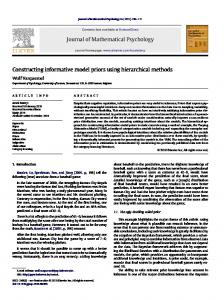
Figure 2: Samples from the joint posterior of range and marginal standard deviation. The red circles are samples using the PC-prior and the black circles are samples using the Jeffreys’ rule prior. because the relative differences are similar. Further, the coverage was further away from the nominal level for the HPD credible intervals than the quantile-based credible intervals for PriorJe and PriorPC, and the coverage of the credible intervals was more sensitive to the hyperparameters of PriorPC for HPD credible intervals than for quantile-based credible intervals. The coverage of the HPD credible intervals was closer to the nominal level than the quantile-based credible intervals for PriorUn1 and PriorUn2, but since our main focus are PriorPC and PriorJe we use the equal-tailed 95% credible intervals in what follows. First, one observation with true range equal to 1.0 is selected and the model is fitted with PriorJe, and with PriorPC with hyperparameters selected such that P(ρ < 0.1) = 0.05 and P(σ > 10) = 0.05. The latter corresponds to a probability of 0.025 that the value of the GRF at an arbitrary location will exceed 10. The resulting samples from the posterior are shown in Figure 2 and the figure shows that when PriorJe is used, the MCMC sampler explores areas far out in the tail, whereas when PriorPC is used, the prior restricts the movement away from the upper tail. This means that when prior knowledge is available, PriorPC can be used to achieve credible intervals that are more reasonable. Second, we study the sensitivity of the coverage and the lengths of the credible intervals to the choice of the hyperparameters in PriorPC and look for general guidelines for selecting the hyperparameters. We choose to set the hyperparameters in PriorPC through P(ρ < ρ0 ) = 0.05 and P(σ > σ0 ) = 0.05. The results show that choosing σ0 lower than the true standard deviation or ρ0 higher than the true range results in too low coverage for both the marginal variance and the range. Selecting σ0 to be 2.5, 10
10
or 40 times the true standard deviation and ρ0 to be 1/10 or 1/2.5 times the true range results in good coverage both for the marginal variance and the range for both values of the true range. Selecting ρ0 to be 1/40 times the true range degrades the coverage for the range when the true range is 0.1, but leads to good coverage when the true range is 1.0, while the coverage for the marginal variance is good for both values of the true range. Thus the study indicates that good coverage properties are achieved when σ0 is selected between 2.5 to 40 times the true standard deviation and ρ0 is set to between 1/10 and 1/2.5 times the true range. Further, shorter credible intervals are achieved for smaller values of σ0 and smaller values of ρ0 , and for the values tested the best balance between good coverage and shortest lengths of the credible intervals is achieved for σ0 equal to 2.5 times the true standard deviation and ρ0 equal to 1/10 times the true range. Third, we compare the properties when using PriorPC, PriorJe, PriorUn1 and PriorUn2. PriorJe results in 98.3% coverage with average length of the credible intervals of 0.78 for range and 96.7% coverage and average length of the credible intervals of 2.6 for marginal variance for true range R0 = 0.1, and 95.6% coverage with average length of the credible intervals of 376 for range and 95.6% coverage with average length of the credible intervals of 295 for variance for R0 = 1. The lengths of the credible intervals are shorter when using PriorPC with the hyperparameters suggested in the previous paragraph than when using PriorJe. The average lengths of the credible intervals are around 1.4 and 3.1 for marginal variance for true ranges 0.1 and 1.0, respectively. Note that the use of HPD intervals significantly reduces the average length of the credible intervals for range and marginal variance for PriorJe to 95 and 75, respectively, but they are still long and there are no hyperparameters that can be used to reduce them. For PriorUn1 the coverage and average lengths of the credible intervals are sensitive to the upper limit on range, and for PriorUn2 the coverage is good and has little sensitivity to the lower and upper limit on range, while the average lengths of the credible intervals are sensitive to the upper limit. Fourth, we investigate whether the behaviour found for PriorPC changes when the observation process is changed to a less informative observation process. For each realization with true range R0 = 0.1 probabilities are calculated through a probit link, probit(pi ) = u(si ), and binomial data is simulated using yi |pi ∼ Binomial(20, pi ). The data is then fitted using the true logistic spatial regression model and the coverage and average lengths of the credible intervals are estimated for marginal variance and range. The results show that the properties found using direct observations of the spatial field also holds for the spatial logistic regression, and the only significant difference is that the average lengths of the credible intervals are larger. Overall, the simulation study shows that with respect to computation time and ease of use versus coverage and lengths of the credible intervals PriorUn2 and PriorPC appear to be the best choices. If coverage is the only concern, PriorUn2 performs the best, but if one also wants to control the length of the credible intervals by disallowing unreasonably high variances, PriorPC offers the most interpretable alternative. Furthermore, choosing the optimal values for σ0 and ρ0 or missing the optimal values by less than one order provides good coverage and lengths of the credible intervals.
11
7300 3.5
7200 3
7100
Northing (km)
7000
2.5
6900 2
6800 1.5
6700 6600
1
6500 0.5
6400
0
200 Easting (km)
400
(a) Observation
(b) Prediction with non-stationary model
Figure 3: Total precipitation for the one year period September 1, 2008, to August 31, 2009, for 233 measurement stations in southern Norway measured in meters in a) and predictions from the non-stationary model in b). Coordinate system is UTM33.
4
Example: Extending to non-stationarity
Neither stationary nor non-stationary GRFs provide true representations of reality, but the extra flexibility in the covariance structure of a non-stationary GRF may provide a better fit to the data than a stationary GRF. Therefore, we consider how to extend the prior for the stationary model to a prior for a non-stationary model, with the goal of improving predictions, using a dataset of annual precipitation. The details are technical and can be found in Appendix G, but this section provides a condensed version. We use a dataset consisting of total annual precipitation for the one year period September 1, 2008, to August 31, 2009, for the 233 measurement stations in southern Norway shown in Figure 3. The dataset has previously been used by Ingebrigtsen et al. (2014, 2015) to study the use of elevation as a covariate in the covariance structure and associated priors. They used an intercept and a linear effect of the elevations of the stations in the first-order structure and used the elevation as a covariate in the secondorder structure. We will follow their choice of covariates in the first-order structure, but use two covariates in the second-order structure: elevation and the magnitude of the gradient of the elevation. We use the simple geostatistical model yi = β0 + xi β1 + u(si ) + �i ,
i = 1, 2, . . . , 233,
(2)
where for station i, yi is the observation made at location si , xi is the elevation of the 12
(a) Elevation (km)
(b) Magnitude of gradient (100m/km)
Figure 4: The covariates (a) elevation and (b) magnitude of the gradient used for the covariance structure. station, (β0 , β1 ) are the coefficients of the fixed effects, u(·) is the spatial effect, and 2 ), and the spatial effect �i is the nugget effect. The nuggets are i.i.d. �i ∼ N (0, σN is constructed with the SPDE approach of Lindgren et al. (2011) and the stationary version has two parameters: spatial range ρ and marginal variance of the spatial field σ 2 . The non-stationary version is constructed as shown in Appendix G and uses the two covariates shown in Figure 4 in the second-order structure. The spatial field is orthogonalized against the intercept and the two covariates in the second-order structure to avoid confounding between the first-order structure and the second-order structure. The stationary model uses the PC prior developed in this paper for the spatial field and the PC prior for precision parameter from Simpson et al. (2017) for the precision of the nugget effect. The hyperparameters are selected to satisfy P(ρ < 10) = 0.05, P(σ > 3) = 0.05 and P(σn > 3) = 0.05, and the model is fitted to the data with INLA (Rue et al., 2009). With this prior we consider a standard deviation greater than 3 large for both the GRF and the nugget effect, and a range less than 10 km unlikely based on the spatial scale that we are working on. The MAP estimates are σ ˆN = 0.13, ρˆ = 219 and σ ˆ = 0.72, and will be used in our scheme for setting the hyperparameters in the prior for the non-stationarity. The non-stationarity is described by a function R(·) that describes how the local range varies and a function S(·) that describes how the marginal variance varies. The two covariates in the second-order linear structure enters linearly in log(R(·)) and log(S(·)), and the coefficients, θ 1 , of the two linear covariates in log(R(·)) are given the prior √ θ 1 |τ1 ∼ N (0, S1 / τ1 ) λ1 −3/2 −λ1 /√τ1 τ1 ∼ τ e 2 1 13
and the coefficients, θ 2 , of the two linear covariates in log(S(·)) are given a similar prior, but with hyperparameter λ2 . Further details are found in Appendix G. The hyperparameters λ1 and λ2 are selected based on the frequentist coverages of the non-stationarity parameters when fitting the non-stationary model to stationary data. Specifically, we use the MAP estimates of the stationary model to simulate 100 datasets from the stationary model with β0 = β1 = 0, set values for the hyperparameters λ1 and λ2 , fit a non-stationary model with β0 = β1 = 0 to each of datasets, and calculate the frequentist coverage of the the 95% credible intervals of the non-stationarity parameters. It is overly expensive to run the model 100 times and we use a cheaper approximation in INLA that is conservative. We tried several values for the hyperparameters λ1 and λ2 and found that λ1 = λ2 = 20 provides coverage that is close to the nominal 95% for θ 1 and θ 2 . The non-stationary model was then fitted using an MCMC sampler and the resulting posterior means of the range and the standard deviation are shown in Appendix G, and they are not included here since the focus is on improving predictions. The figures show that the non-stationary model moves away from the stationary model even under the conservative prior. The leave-one-out log-score is estimated from the samples of the MCMC sampler, and we find the score 0.13 for the stationary model and 0.22 for the non-stationary model. The leave-one-out estimates for the continuous rank probability score (CRPS) are 0.092 for the stationary model and 0.083 for the non-stationary model. Experimentation with the strictness of the prior showed that further improvements were possible by making the prior weaker, but that making the prior too weak leads to worse scores. The prior and the procedure for selecting the hyperparameters appears to introduce a reasonable level of conservativeness for this dataset. If we run the model with the same hyperparameters and remove the non-stationarity in the local range, the CRPS is 0.086, and if we remove the non-stationarity in the marginal standard deviations, the CRPS is 0.081. This shows that the covariates in the local range appear to be contributing more to the improved predictions than the covariates in the standard deviation, and that using all four covariates has degraded the performance slightly compared to using only a non-stationary local range. This demonstrates that guaranteeing improvements when including more covariates in the second-order structure is difficult. So a procedure for constructing conservative priors are critically important for non-stationary models, but the prediction scores of the models must be compared to ensure that the non-stationary model improves the predictions.
5
Discussion
The main challenge for constructing multivariate PC priors based on a measure of distance from a base model is that a joint prior for the parameters cannot be uniquely determined from a prior for the distance. Simpson et al. (2017) present a general approach where conditional on the value of the distance, D, the probability density is uniformly distributed on the set of parameters that specify models that are a distance 14
D from the base model, but the approach is not parametrization-invariant and it is not clear for which parametrization of range and marginal variance that this approach would be appropriate. However, in this paper we have shown that the key for properly extending the PC prior framework to a joint prior for range and marginal variance in Matérn GRFs with fixed smoothness is to use knowledge about the parameter space to split the construction of the multivariate PC prior into a sequential construction of univariate PC priors. This demonstrates that the principles of the PC prior framework are applicable for model components with complex parameter spaces that contain intrinsically linked parameters, but that the simple idea of distance from a base model must be combined with careful consideration of the parameter space. The construction of the joint prior based on the infinite-dimensional distribution of the GRF instead of the finite-dimensional distribution of an observation from the GRF is technically more challenging that the finite-dimensional examples in Simpson et al. (2017). But the calculation of the KLD can be handled using the spectrum of the GRF and the fact that the KLD is infinite for general changes in the parameters can be overcome by careful reparametrization and a sequential construction of the prior. The benefits gained from the extra difficulty are that the PC prior for Matérn GRFs with fixed smoothness and the extension to the non-stationary GRF are computationally inexpensive since they have simple forms, are appropriate for hierarchical models since they work with any observation process, and can be applied for sequential analysis of data since they do not depend on the design of the experiment. Setting the hyperparameters for the stationary part of the model can be done based on statements about what constitutes a large standard deviation or a large deviation from zero for the spatial field, and what constitutes a small range. This allows the users to choose to limit the preference for intrinsic models and thus provide more sensible posterior inference for the problem at hand. In the simulation study we observe good coverage of the equal-tailed 95% credible intervals when the prior satisfies P(σ > σ0 ) = 0.05 and P(ρ < ρ0 ) = 0.05, where σ0 is between 2.5 to 40 times the true marginal standard deviation and ρ0 is between 1/10 and 1/2.5 of the true range. The lengths of the credible intervals depend on the values chosen for σ0 and ρ0 , but are shorter than for the reference prior and consistent with the information put into the prior. The recommendations are based on the quantile-based credible intervals because the coverage of the 95% HPD credible intervals is further away from the nominal level and more sensitive to hyperparameters than the equal-tailed 95% credible intervals when the PC prior is used. It is difficult to elicit expert knowledge about the hyperparameters for a non-stationary GRF since the second-order structure is not observed directly, and we discuss an alternative way to set the hyperparameters based on the frequentist coverage of the credible intervals. Using the new prior and the associated scheme for selecting the hyperparameters, we find a better fit for the non-stationary GRF than with the stationary GRF when applied to the dataset of annual precipitation in southern Norway measured both with leave-one-out CRPS and log scores. The paper shows that the PC prior framework provides a useful tool for deriving a
15
principled joint prior for the range and the marginal variance of a Matérn GRF with fixed smoothness, and that the ideas of the framework are useful for constructing priors that limit flexibility also for non-stationary GRFs where exact derivation is not possible.
A A.1
Proofs Theorem 2.1
Proof. For a fixed value of κ, the covariance matrix of u = (u(s1 , u(s2 ), . . . , u(sn )) is Σ(τ ) = τ 2 Σ0 , where Σ0 depends on the values of κ and ν and the locations at which the process is observed. This means that u|τ, κ ∼ Nn (0, τ 2 Σ0 ), and we need to derive the PC prior for the scale parameter of a multivariate Gaussian distribution with the base model τ = 0. This can be formulated as constructing the PC prior for a precision parameter, which was done in Simpson et al. (2017, Appendix A.2), and a transformation to a scale parameter results in π(τ |κ) = λ exp(−λτ ), for τ > 0, where λ > 0.
A.2
Theorem 2.2
Proof. The marginal standard deviation is given by σ = τ κ−ν C −1 , where s Γ(ν + d/2)(4π)d/2 C= . Γ(ν) The probability P(σ > σ0 |κ) = α is equivalent to P(τ > σ0 κν C|κ) = α and under the prior distribution this leads to exp(−λσ0 κν C) = α s λ = −κ−ν
A.3
Γ(ν) log(α) . d/2 σ0 Γ(ν + d/2)(4π)
Theorem 2.3
Proof. Restrict u to the subset [0, L]d ⊂ Rd and let κ = κ0 > 0 denote the base model. Let 1/L = o(κ0 ), then the covariance function on [0, L]d is, for small κ0 , well approximated by � �d X 2π , c(s, t) = fν (w; κ, τ ) exp (−ıhw, s − ti) L 2π d w∈
L
Z
where fν (w; κ, τ ) = (2π)−d τ 2 (κ2 + ||w||2 )−(ν+d/2) is the spectral density of a Matérn GRF on Rd with parameters τ , κ and ν (See Lindgren et al. (2011)). Further, the KLD
16
for the periodic approximation from κ0 to κ, for a fixed τ , is (based on Bogachev (1998, Thm. 6.4.6)) � � 1 X fν (w; κ, τ ) fν (w; κ, τ ) KL(κ, κ0 ) = − 1 − log 2 fν (w; κ0 , τ ) fν (w; κ0 , τ ) 2π d w∈
=
1 2
L
Z
� X � (κ2 + ||w||2 )α (κ20 + ||w||2 )α 0 − 1 − log , (κ2 + ||w||2 )α (κ2 + ||w||2 )α 2π d
w∈
L
Z
where α = ν + d/2. The sum can be divided in two parts: the zero frequency E0 and the other frequencies E1 . The zero frequency term is �� 2 �α � 2 �α � 1 κ0 κ0 E0 = − 1 − log 2 2 κ κ2 and the remaining terms are � � � � � �d X ((κ0 /κ)2 + ||w||2 )α ((κ0 /κ)2 + ||w||2 )α 2π 1 Lκ d − 1 − log E1 = 2 )α 2 )α 2 2π (1 + ||w|| (1 + ||w|| Lκ 2π d w∈ Lκ Z ,w6=0
1 = 2
�
Lκ 2π
� d �Z
�
Rd
� � ((κ0 /κ)2 + ||w||2 )α ((κ0 /κ)2 + ||w||2 )α − 1 − log dw + o(1) (1 + ||w||2 )α (1 + ||w||2 )α
as κ0 → 0. For any fixed value of L, we may include (L/(2π))d in the hyperparameter λ in the PC prior. Thus we consider the rescaled terms � �d �� 2 �α � 2 �α � κ0 κ0 ˜0 = 1 2π E − 1 − log 2 L κ κ and ˜1 = 1 κd E 2
�Z Rd
�
� � ((κ0 /κ)2 + ||w||2 )α ((κ0 /κ)2 + ||w||2 )α − 1 − log dw + o(1) . (1 + ||w||2 )α (1 + ||w||2 )α
˜0 → 0 and, for d ≤ 3, Let κ0 → 0 with 1/L = o(κ0 ), then E � � �α � Z �� α 1 d ||w||2 ||w||2 1 ˜ − 1 − log dw = Cα κd , E1 → κ 2 2 2 (1 + ||w|| ) (1 + ||w|| ) 2 Rd where the finiteness of the integral is shown to hold in Appendix H, and Cα is a constant that depends on α and d. q ˜ The distance from the base model is dist(κ) = 2 · 1 Cα κd , where we can absorb the 2
constants in the hyperparameter of the PC prior, so we choose the distance dist(κ) = κd/2 . The PC prior using an exponential distribution on the distance is then π(κ) = λ exp(−λκd/2 )
d d/2 dλ d/2−1 κ = κ exp(−λκd/2 ), dκ 2
17
κ > 0.
A.4
Theorem 2.4
√ Proof. The probability P(ρ < ρ0 ) = α is equivalent to P(κ > 8ν/ρ0 ) = α and under the prior distribution we find √ exp(−λ( 8ν/ρ0 )d/2 ) = log(α) � � ρ0 d/2 λ=− √ log(α). 8ν
A.5
Theorem 2.5
Proof. Using Theorems 2.1 and 2.3, we find the joint prior π(κ, τ ) = π(κ)π(τ |κ) d = λ1 κd/2−1 exp(−λ1 κd/2 )λ2 exp(−λ2 τ ) 2 d = λ1 λ2 κd/2−1 exp(−λ1 κd/2 − λ2 τ ), τ > 0, κ > 0. 2 And Theorems 2.2 and 2.4 gives � λ1 = −
A.6
ρ √0 8ν
s
�d/2 log(α1 ) and λ2 = −κ
−ν
Γ(ν) log(α2 ) . Γ(ν + d/2)(4π)d/2 σ0
Theorem 2.6
Proof. Since there is no dependence of ρ on √ τ , the change of variables from (κ, τ ) to (ρ, σ) can be divided in two steps. First, ρ = 8ν/κ so we find √ d√ −1 π(ρ) = π(κ = 8ν/ρ) 8νρ dρ √ d/2−1 −d/2+1 √ √ d = λ1 ( 8ν) ρ exp(−λ1 ( 8ν)d/2 ρ−d/2 ) 8νρ−2 2 d ˜ −d/2−1 ˜ 1 ρ−d/2 ), ρ > 0, = λ1 ρ exp(−λ 2 d/2
˜ 1 = − log(α1 )ρ . where λ 0 Second, σ = τ κ−ν C −1 , where s C=
Γ(ν + d/2)(4π)d/2 . Γ(ν)
18
Note that conditioning on κ is equivalent to conditioning on ρ. So the density π(σ|ρ) can be found by ∂ ν ν π(σ|ρ) = π(σ|κ) = π(τ = σκ C|κ) σκ C ∂σ = λ2 exp(−λ2 σκν C)κν C ˜ 2 exp(−λ ˜ 2 σ), σ > 0, =λ ˜ 2 = − log(α2 ) . So the joint density is where λ σ0 π(ρ, σ) = π(ρ)π(σ|ρ) =
B
d ˜ ˜ −d/2−1 ˜ 1 ρ−d/2 − λ ˜ 2 σ), λ1 λ2 ρ exp(−λ 2
ρ > 0, σ > 0.
Detailed discussion for bounded domains
The derivations in the main paper use the assumption that the size of the domain is large compared to the range of the base model. This is a reasonable assumption if the underlying GRF exists on a larger domain than the area on which observations have been made since the prior should be based on the distribution of the GRF on the domain where it is defined. However, if it is known that the GRF only exists on a bounded domain, it would be reasonable to base the derivation instead on the bounded domain and not a larger ambient domain. When the parameter κ increases, the variance of the process increases, but the spread of the observations relative to each other does not change. Since there is no larger ambient space in which this effect could be distinguished from adding an intercept to the model, it is more meaningful to have a base model with finite range. When the priors are derived based on bounded domains, there will typically not be any analytic expressions available. One exception is the exponential covariance function on the one-dimensional domain [0, L] where the exact expression for the distance between the models specified by (κ, τ ) and (κ0 , τ ) can be derived (see Section C) and is given by s � 2 � �κ � κ0 κ0 κ 0 dist1D,exp (κ||κ0 ) = − 1 − log +L − κ0 + . (3) κ κ 2κ 2 √ In this case it is clear that the term log(κ) dominates when κ is small if 8ν/κ0 is of the same order as L or larger. In the following example one can see how the prior for κ calculated based on this distance differs from the one derived in the previous section Example B.1 (One-dimensional exponential covariance function). Let a GRF with an exponential covariance function be observed on [0, 1]. There is a one-to-one correspondence between κ and ρ, so the distance given in Equation (3) can be expressed in range by s � � � � √ ρ ρ ρ 1 1 distρ0 (ρ) = − 1 − log + 8ν − + , ρ0 ρ0 2ρ20 ρ0 2ρ 19
1.5 1.0
Probability density
0.0
0.5
1.5 1.0
Probability density
0.5 0.0 0.0
0.5
1.0
1.5
2.0
0
1
rho
2
3
4
rho
(a) Base model ρ0 = 2
(b) Base model ρ0 = 4
Figure 5: The PC prior based on the unbounded domain is shown as dashed lines in each subfigure and the prior based on the bounded domain is shown as solid lines for base model (a) ρ0 = 2 (b) ρ0 = 4. The prior based on the unbounded domain continues to ρ = ∞. where ρ0 is the range of the base model. This distance results in the prior √ � �! 1 8ν 1 1 1 1 π1 (ρ) = λ1 exp(−λ2 distρ0 (ρ)) − + − , 0 < ρ < ρ0 , 2distρ0 (ρ) ρ ρ0 2 ρ2 ρ20 where λ1 = − log(α)/distρ0 (R0 ) ensures that P(ρ < R0 ) = α. For comparison, the prior for ρ based on an unbounded domain is π2 (ρ) =
λ2 −3/2 ρ exp(−λ2 ρ−1/2 ), 2
ρ > 0,
1/2
where λ2 = − log(α)R0 ensures that P(ρ < R0 ) = α. The parameter values R0 = 0.05 and α = 0.05 are chosen, and the prior based on the unbounded domain and the priors based on the bounded domain for ρ0 = 2 and ρ0 = 4 are shown in Figure 5. The figure shows that the two prior constructions are similar for ρ < 0.25 for ρ = 2 and for ρ < 0.5 for ρ0 = 4. For higher values of range, π2 distributes the probability mass over the entire positive line and has a faster decay than π1 . The priors will not correspond to each other in the case that ρ0 → ∞. In that case π1 will have a decay of approximately 1/ρ whereas π2 has a decay of approximately ρ−3/2 . For other covariance functions and for bounded domains of dimension 2 and 3, the analytic expressions for the distances are not known, but the priors can be approximated 20
numerically. The values of the prior on an interval κ ∈ [A, B] can be computed by selecting a grid of sufficiently dense locations in the domain and then calculating the KLD based on this finite set of locations. It would be possible to use a fully design-dependent prior where the KLD is calculated based on the observation locations in the dataset of interest, but this provides, potentially, undesired behaviour. Even for a bounded domain one is interested in doing predictions outside the observed locations on a much higher resolution and in that case using a prior that ignores all properties of the higher resolution process would not be advisable. If one wants to be able to do predictions at arbitrarily high resolution, the prior should be constructed based on the infinite-dimensional GRF defined on the full bounded domain. The following example demonstrates how calculations may be done in the two-dimensional case and the consequence of using a too low resolution in the calculation of the prior. Example B.2 (Two-dimensional Matérn covariance function with ν = 3/2). Let a GRF with a Matérn covariance function with smoothness ν = 1.5 be observed on [0, 1]2 , and let the base model be given by ρ0 = 4. We calculate priors π1 , π2 and π3 for the range based on a regular grid of 10 × 10 points, 20 × 20 points and 40 × 40 points, respectively, and prior π4 , which is the prior calculated based on an unbounded domain. For each prior the hyperparameter is set such that P (ρ < 0.05) = 0.05. The calculated priors are shown in Figure 6 and demonstrate that the lower tail behaviour varies strongly dependent on the number of locations used to calculate the PC prior. One can see that the lower the resolution is, the higher the values of the prior in the left-hand side tail. Intuitively, this is because the distance decreases more slowly as a function of range as range goes to zero the lower the resolution is, and this causes more probability mass to be placed further out in the tail. This is because most of the differences in the GRFs for low ranges cannot be detected when it is observed at lower resolution. However, since the properties of the prior are used when making predictions at higher resolutions, we suggest to use the prior based on the continuous process instead of the discrete observation process. As the resolution of the grid used to calculate the prior using the bounded domain goes to infinity, the prior will agree better and better with the prior based on the unbounded domain for low values of the range. In Example B.1 the overlap for low values of range is clear since the analytic expression for infinite resolution is used. Even though there are cases in which the domain of the GRF is naturally limited to the area on which the observations are made, the use of priors based on an unbounded domain have many advantages. The priors based on the bounded domain are more expensive to calculate and require the additional choice of a range for the base model, but have the same lower tail behaviour as the prior based on the unbounded domain and only the behaviour for higher ranges changes. Overall, we find that the unbounded domain prior is most appealing.
21
1e+01
4
1e−01 1e−05
1e−03
Probability density
3 2
Probability density
1 0 0
1
2
3
4
1e−06
rho
1e−04
1e−02
1e+00
rho
(a) Original axes
(b) Log-log axes
Figure 6: PC priors for range in a Matérn GRF observed on [0, 1]2 with smoothness ν = 3/2. The prior based on the unbounded domain is shown as dash-dot-dashed line, and the priors for the bounded domain based on 10×10 points, 20×20 points and 40×40 are shown as a solid line, a dashed line and a dotted line, respectively. For each of the priors based on bounded domains the base model is ρ0 = 4.
C C.1
Distance for exponential covariance function on bounded one-dimensional domain Goal
Let uκ be a stationary GRF with the exponential covariance function, c(d) =
1 −κd e , 2κ
(4)
where κ > 0. This way of writing the exponential covariance function differs from the traditional parametrization using the range and the marginal variance, and is chosen because the KLD between the distributions described by different values κ > 0 is finite. The parametrization describes how to move in the parameter space while keeping the KLD finite. The goal of this appendix is to calculate the KLD between the distributions of uκ and uκ0 on the interval [0, L]
C.2
Discretization
The direct computations for the interval [0, L] are difficult. So we first consider the KLD for the distributions of uκ and uκ0 at the observation points ti = i∆t, for i = 0, 1, . . . , N , where ∆t = L/N . The spatial field uκ can be described as a stationary solution of the
22
stochastic differential equation duκ (t) = −κuκ (t)dt + dW (t), where W is a standard Wiener processes, and written explicitly as Z t e−κ(t−s) dW (s). uκ (t) = −∞
This expression shows that uκ (ti+1 )|uκ (ti ) ∼ N (e−κ∆t uκ (ti ), σκ2 ), where σκ2
Z
t+∆t
= Var[uκ (t + ∆t)|uκ (t)] =
e−2κ(t+∆t−s) ds =
t
1 − e−2κ∆t . 2κ
This is an AR(1) process with initial condition uκ (t0 ) ∼ N (0, (2κ)−1 ), which means that uκ = (uκ (t0 ), . . . , uκ (tN )) has a multivariate Gaussian distribution with mean 0 and precision matrix 1 −e−κ∆t −e−κ∆t 1 + e−2κ∆t −e−κ∆t 1 . . . .. .. .. Qκ = 2 (5) . σκ −κ∆t −2κ∆t −κ∆t −e 1+e −e −κ∆t −e 1
C.3
Kullback-Leibler divergence
The vectors uκ0 and uκ have multivariate Gaussian distributions and the KLD from the distribution described by κ0 to the distribution described by κ is � �� � 1 |Qκ0 | −1 KL(κ, κ0 ) = tr(Qκ0 Qκ ) − (N + 1) − log . 2 |Qκ | We are interested in taking the limit ∆t → 0 to find the value corresponding to the KLD from uκ0 to uκ . This is done in two steps: first we consider the trace and the N + 1 term, and then we consider the log-determinant term. C.3.1
Step 1
Let fκ = 1/σκ2 , then the trace term can be written as tr(Qκ0 Σκ ) " = fκ0 2cκ (0) +
N −1 X
N X
i=1
i=1
(1 + e−2κ0 ∆t )cκ (0) − 2
# e−κ0 ∆t cκ (∆t)
� � = fκ0 2cκ (0) + (N − 1)(1 + e−2κ0 ∆t )cκ (0) − 2N e−κ0 ∆t cκ (∆t) .
23
We extract the first summand and parts of the last summand, and combine with 2 from the N + 1 term, to find the limit 1 − e−(κ+κ0 )∆t −2 2κ κ + κ0 fκ0 /∆t −2 = κ fκ+κ0 /∆t κ0 − κ → . κ For the remaining summands and the remaining N − 1 from the N + 1 term, we can simplify the expression as 2fκ0 [cκ (0) − e−κ0 ∆t cκ(∆t)] − 2 = 2fκ0
S3 (∆t) � � 1 + e−2κ0 ∆t cκ (0) − 2e−κ0 ∆t cκ (∆t) − (N − 1) " # � e−(κ0 +κ)∆t −2κ0 ∆t 1 = (N − 1)fκ0 1 + e − (N − 1) −2 2κ 2κ � 1 4κ2 (∆t)2 = (N − 1)fκ0 1 + (1 − 2κ0 ∆t + 0 ) 2κ 2 � (κ0 + κ)2 (∆t)2 2 − 2(1 − (κ0 + κ)∆t + ) + o((∆t) ) − (N − 1) 2 � 1 = (N − 1)fκ0 (−2κ0 + 2(κ0 + κ))∆t 2κ � 2 2 2 2 + (2κ0 − (κ0 + κ) )(∆t) + o((∆t) ) − (N − 1) � � 2κ20 − (κ0 + κ)2 2 2 (∆t) + o((∆t) ) − (N − 1) = (N − 1)fκ0 ∆t + 2κ � �� �� L 1 = −1 + κ0 + o(1) ∆t ∆t ∆t � � � 2κ20 − (κ0 + κ)2 L 2 2 (∆t) + o((∆t) ) − −1 , + 2κ ∆t = (N − 1)fκ0
�
and see that the products involving o(1) tend to zero � � 1 2κ20 − (κ0 + κ)2 1 S3 (∆t) = L + − + Lκ0 − [1 + o(1)] + 1 ∆t 2κ ∆t 4κ2 − (κ0 + κ)2 + Lκ0 + o(1) =L 0 2κ � � κ20 κ = L κ0 + − κ0 − + o(1). 2κ 2 Thus the limit is κ0 tr(Qκ0 Σκ ) − (N + 1) → −1+L κ 24
�
κ20 κ − 2κ 2
� .
C.3.2
Step 2
The determinant of the matrix in Equation (5) can be found by summing rows upwards, and we see that |Q| = σ −2(N +1) (1 − e−2κ∆t ) = 2κσ −2N . Note that in the limit κ → 0, f → ∆t so the determinant behaves asymptotically as κ. This means that ! � � 2κ0 fκN0 |Qκ0 | log = log |Qκ | 2κfκN � � �κ � fκ0 0 = log + N log κ fκ and we need to find the limit of the second part, � � fκ0 N log fκ � � L 1 1 = − log log ∆t fκ fκ0 � � � � �� � � L 1 1 −2κ∆t −2κ0 ∆t = log 1−e − log 1−e ∆t 2κ 2κ0 � �� L � = log ∆t − κ(∆t)2 + o((∆t)2 ) − log ∆t − κ0 (∆t)2 + o((∆t)2 ) ∆t L = [log (1 − κ∆t + o(∆t)) − log (1 − κ0 ∆t + o(∆t))] ∆t L [−κ∆t + κ0 ∆t + o(∆t)] = ∆t Thus the limit is
� log
C.4
|Qκ0 | |Qκ |
� → log
�κ � 0
κ
+ L(κ0 − κ)
Full KLD
The combination of the limits from the two steps gives the full KLD, � � 2 � � �κ � 1 κ0 κ0 κ 0 KL(κ, κ0 ) = −1+L − − log − L(κ0 − κ) 2 κ 2κ 2 κ � � �� �κ � 1 κ0 κ20 κ 0 = − 1 − log +L − κ0 + . 2 κ κ 2κ 2
D
(6)
Details for the simulation study
In this section we present a small simulation study of the frequentist coverage of the credible intervals for the range and the marginal variance, and the behaviour of the joint 25
1.0 0.8 0.6 0.4 0.2 0.0 0.0
0.2
0.4
0.6
0.8
1.0
Figure 7: Spatial design for the simulation study. posterior when using the PC prior, the Jeffreys’ rule prior, and the Jeffreys prior for variance combined with a bounded uniform prior on range and a bounded uniform prior on the logarithm of range.
D.1
Study setup
We choose the observation domain [0, 1]2 ⊂ R2 and select the 25 observation locations, s1 , s2 , . . . , s25 , shown in Figure 7 at random. Then we simulate observations, u = (u(s1 ), u(s2 ), . . . , u(s25 )), for these observation locations for a GRF with an exponential covariance function c(r) = exp(−2r/R0 ) for R0 = 0.1 and R0 = 1. We generate 1000 realizations of the observations for R0 = 0.1 and R0 = 1 and collect them in datasets Data1 and Data2 , respectively. Additionally, for each of the 1000 realizations in Data1 a third dataset (Data3) is generated by simulating yi |pi ∼ Binomial(20, pi ), where probit(pi ) = ui , for i = 1, 2, . . . , 25. Two models are used to fit the data: a spatial regression model (Model1) and a spatial logistic regression model (Model2). In Model1 observations are modelled as yi = u(si ), for i = 1, 2, . . . , 25, where u is an exponential GRF with the covariance function, c(r) = σ 2 exp(−2r/ρ), where σ 2 is the marginal variance and ρ is the range, and in Model 2 the observations are modelled as yi |pi ∼ Binomial(20, pi ), where probit(pi ) = u(si ), for i = 1, 2, . . . , 25, where u is an exponential GRF with covariance function, c(r) = σ 2 exp(−2r/ρ), where σ 2 is the marginal variance and ρ is the range. Four different priors are used for the parameters: the PC prior (PriorPC), the Jeffreys’ rule prior (PriorJe), a uniform prior on range on a bounded interval combined with the Jeffreys’ prior for variance (PriorUn1) and a uniform prior on the log-range on a bounded interval combined with the Jeffreys’ prior for variance (PriorUn2). The full expressions for the priors are given in Table 1. 26
Table 1: The four different priors used in the simulation study. The Jeffreys’ rule prior ∂ uses the spatial design of the problem through U = ( ∂ρ Σ)Σ−1 , where Σ is the correlation matrix of the observations (See Berger et al. (2001)). Prior
Expression
PriorPC
π1 (ρ, σ) = λ1 λ2 ρ−2 exp −λ1 ρ−1 − λ2 σ
−1
�
1 tr(U ) − tr(U )2 n 2
�1/2
�
Parameters ρ, σ > 0 Hyperparameters: αρ , ρ0 , ασ , σ0
ρ, σ > 0 Hyperparameters: None
PriorJe
π2 (ρ, σ) = σ
PriorUn1
π3 (ρ, σ) ∝ σ −1
ρ ∈ [A, B], σ > 0 Hyperparameters: A, B
PriorUn2
π4 (ρ, σ) ∝ σ −1 · ρ−1
ρ ∈ [A, B], σ > 0 Hyperparameters: A, B
27
D.2
Frequentist coverage
The series of papers on reference priors for GRFs starting with Berger et al. (2001) evaluated the priors by studying frequentist properties of the resulting Bayesian inference. A prior intended for use as a default prior should lead to good frequentist properties such as frequentist coverage of the equal-tailed 100(1 − α)% Bayesian credible intervals that is close to the nominal 100(1 − α)%. In this paper, the study is replicated with one key difference: no covariates are included. This choice is made because the PC prior is derived for a zero-mean GRF, and if a mean were desired, it would be handled by extending the hierarchical model with another latent component that had its own, separate prior. Without covariates the reference prior approach results in the Jeffreys’ rule prior as there are no nuisance parameters to integrate out when constructing the spatial reference prior. Furthermore, we compute the 100(1 − α)% highest posterior density (HPD) credible intervals (Chen and Shao, 1999) since the resulting posteriors will be highly skewed and the HPD intervals may differ substantially from the quantilebased intervals. In this section Model1 is combined with PriorJe, PriorPC, PriorUn1 and PriorUn2. Data1 and Data2 each contains 1000 realizations and the frequentist coverage is estimated for the equal-tailed 95% credible intervals and the HPD 95% credible intervals for the range and the marginal variance by counting how many times the true parameter value is included in the credible intervals. The equal-tailed intervals are calculated based on the quantiles of the samples from an MCMC chain and the HPD intervals are calculated using the BOA package (Smith et al., 2007). We split the presentation of the results for the quantile-based credible intervals and the HPD credible intervals: in this section we discuss the quantile-based intervals and their associated results, and in the next section we discuss the results for the HPD credible intervals and differences from the results for the quantile-based intervals. PriorJe has no hyperparameters, but PriorPC, PriorUn1 and PriorUn2 each has hyperparameters that need to be set before using the priors. For PriorUn1 and PriorUn2 it is hard to give guidelines about which values should be selected since the main purpose of limiting the prior distributions to a bounded interval is to avoid an improper posterior and the choice tends to be ad-hoc. For PriorPC, on the other hand, there is an interpretable statement for selecting the hyperparameters, which helps give an idea about which prior assumptions the chosen hyperparameters are expressing. For PriorPC we need to make an a priori decision about the scales of the range and the marginal variance. The prior is set through four hyperparameters that describe our prior beliefs about the spatial field. We use P(ρ < ρ0 ) = 0.05 for ρ0 = 0.025ρT , ρ0 = 0.1ρT , ρ0 = 0.4ρT and ρ0 = 1.6ρT , where ρT is the true range. This covers a prior where ρ0 is much smaller than the true range, two priors where ρ0 is smaller than the true range, but not far away, and one prior where ρ0 is higher than the true range. For the marginal variance we use P(σ 2 > σ02 ) = 0.05, for σ0 = 0.625, σ0 = 2.5, σ0 = 10 and σ0 = 40. We follow the same logic as for range and cover too small and too large σ0 and two reasonable values. For PriorUn1 and PriorUn2, we set the lower and upper limits for the nominal range according to the values A = 0.05, A = 0.005 and A = 0.0005, and 28
Table 2: Frequentist coverage of the 95% credible intervals for the range and the marginal variance when the true range is ρT = 0.1 using PriorPC. The average lengths of the credible intervals are shown in brackets. (a) Range
ρ0 \σ0
40
0.0025 0.01 0.04 0.16
0.755 0.969 0.988 0.723
10 [0.24] [0.33] [0.46] [0.99]
0.776 0.970 0.990 0.685
2.5 [0.22] [0.32] [0.41] [0.82]
0.760 0.958 0.991 0.733
0.625 [0.20] [0.28] [0.33] [0.55]
0.709 0.924 0.990 0.798
[0.18] [0.21] [0.25] [0.34]
(b) Marginal variance
ρ0 \σ0
40
0.0025 0.01 0.04 0.16
0.960 0.934 0.949 0.895
10 [1.5] [1.6] [2.0] [3.8]
0.943 0.966 0.945 0.905
2.5 [1.4] [1.6] [1.8] [3.2]
0.946 0.960 0.953 0.947
0.625 [1.3] [1.4] [1.5] [2.2]
0.898 0.923 0.941 0.977
[0.97] [0.99] [1.1] [1.3]
B = 2, B = 20 and B = 200. Some of the values are intentionally extreme to see the effect of misspecification. The results for PriorPC are given in Tables 2 and 3 for the true ranges ρT = 0.1 and ρT = 1, respectively, and the tables for PriorUn1 and PriorUn2 are given in Section E. PriorJe resulted in 98.3% coverage with average length of the credible intervals of 0.78 for range and 96.7% coverage and average length of the credible intervals of 2.6 for marginal variance for ρT = 0.1, and 95.6% coverage with average length of the credible intervals of 376 for range and 95.6% coverage with average length of the credible intervals of 295 for variance for ρT = 1. The tables show that for PriorPC, PriorUn1 and PriorUn2 the coverage and the length of the credible intervals are sensitive to the choice of hyperparameters. The lengths of the credible intervals are, in general, more well-behaved for ρT = 0.1 than for ρT = 1 because there is more information about the range available in the domain when the range is shorter. The results verifies the observations by Berger et al. (2001) that the inference is overly sensitive to the hyperparameters for PriorUn1. The coverage and the length of the credible intervals are strongly dependent on the upper limit of the prior. For PriorUn2 the coverage is good in both the short range and long range case, but the length of the credible intervals are sensitive to the upper limit of the prior. For PriorJe the coverage is good, but the credible intervals are excessively long and the prior is computationally expensive and only computationally feasible for a low number of observation locations. The average length of the credible intervals for ρT = 1 for marginal variance is 295, which imply unreasonably high standard deviations. The high standard deviations do not seem consistent with observations drawn with true marginal variance equal to 1. Further, the results show that the coverage for PriorPC is stable when a too low 29
Table 3: Frequentist coverage of the 95% credible intervals for the range and the marginal variance when the true range is ρT = 1 using PriorPC. The average lengths of the credible intervals are shown in brackets. (a) Range
ρ0 \σ0
40
10
0.025 0.1 0.4 1.6
0.957 [12] 0.977 [14] 0.963 [25] 0.63 [73]
0.947 0.967 0.970 0.301
2.5 [7.3] [8.5] [13] [32]
0.921 0.962 0.988 0.711
0.625 [3.3] [3.5] [5.2] [11]
0.782 0.861 0.980 0.945
[1.4] [1.5] [1.9] [3.3]
(b) Marginal variance
ρ0 \σ0
40
0.025 0.1 0.4 1.6
0.956 0.964 0.953 0.435
10 [11] [13] [22] [69]
0.949 0.966 0.964 0.549
2.5 [6.5] [7.5] [12] [29]
0.927 0.950 0.980 0.804
0.625 [2.8] [3.1] [4.5] [9.1]
0.771 0.848 0.965 0.988
[1.1] [1.2] [1.5] [2.5]
lower limit for range or a too high upper limit for marginal variance is specified, but that specifying a too high lower limit for the range or a too low upper limit for variance produces large changes in the coverage. This is not unreasonable as the prior is then explicitly stating that the true value for range or variance is unlikely. The average length of the credible intervals are more sensitive to the hyperparameters than the coverages, but we see less extreme sizes for the credible intervals than for PriorJe. With respect to computation time and ease of use versus coverage and length of credible intervals PriorUn2 and PriorPC appear to be the best choices. If coverage is the only concern, PriorUn2 performs the best, but if one also wants to control the length of the credible intervals by disallowing unreasonably high variances, PriorPC offers the most interpretable alternative. In a realistic situation it is highly likely that the researcher has prior knowledge, for example, that the spatial effect should not be greater than, say 4, and by encoding this information in PriorPC one can limit the upper limits of the credible intervals both for range and marginal variance.
D.3
Differences in results between equal-tailed and HPD credible intervals
For each case discussed in the previous section, we also calculated the 95% credible intervals using HPD intervals and the results and tables are found in Section F. In general, the average length of the credible intervals are significantly shorter for HPD credible intervals than for quantile-based credbile intervals, and the most substantial decrease is seen for true range equal to 1.0 using PriorJe, where the average length of the credible interval decreases from 376 to 95 for range and from 295 to 75 for marginal 30
variance. However, the conclusions in the previous section on differences in average lengths of credible intervals between priors and between true range equal to 0.1 and 1.0 remain valid since the relative differences remain similar. In particular, the average length of the HPD credible intervals for marginal variance for PriorJe with true range equal to 1.0 is around 95, which is still unreasonably high when prior knowledge about the marginal standard deviation is available. The coverage of the credible intervals constructed using HPD intervals differ from the quantile-based intervals. For PriorPC, the coverage of the HPD intervals is more sensitive to the hyperparameters and if ρ0 = 0.4ρT the coverage of the HPD intervals for range are almost 100%. Further, the coverage of the HPD intervals for marginal variance are excessively high when σ0 = 40 or σ0 = 10, and there is no recommendation for hyperparameters that perform consistently well in both true range equal to 0.1 and 1.0 and for both range and marginal variance. Similarly, the coverage of the credible interval for range is almost 100% when the true range is 0.1 with PriorJe. This contrasts the quantile-based credible intervals where PriorJe performs well with respect to coverage for both true range equal to 0.1 and 1.0. For PriorUn1 and PriorUn2 the coverage of the HPD credible intervals are less sensitive to hyperparameters than the quantile-based credible intervals, but the the HPD intervals tend to have higher coverage than the nominal level. We use the equal-tailed 95% credible intervals in what follows since the 95% HPD credible intervals are further away from nominal level and more sensitive to hyperparameters than equal-tailed 95% credible intervals for the PC prior.
D.4
Behaviour of the joint posterior
In the previous section we only studied the marginal properties of the posterior, but these do not tell the entire story because there is strong dependence between the range and the marginal variance in the posterior distribution. We study this dependence using one realization from Data2 where the true range is 1 and the observed values lie in the range −1 to 3. An MCMC sampler is used to draw samples from the posterior of the marginal standard deviation and the range. Model1 is combined with PriorJe, and PriorPC with hyperparameters αρ = 0.05, ρ0 = 0.1, ασ = 0.05 and σ0 = 10. Figure 8 shows the strong posterior dependence between the marginal standard deviation and the range in the tail of the distribution. The long tails are not a major concern for predictions since the asymptotic predictions are the same along the ridge, but they pose a concern for the interpretability of the range and the marginal variance. Since the values of the observations lie within the range −1 to 3, it is unlikely that the true standard deviation should be on the order of 20. As seen in Figure 9, the heavier upper tail for the joint posterior when using PriorJe compared to using PriorPC results in heavier tails also for the marginal posteriors. The lower endpoints of the equal-tailed credible intervals are similar using both priors, but there is a large difference in the upper endpoints. The PC prior for range has a heavy upper tail and the upper tail of the posterior for the range is controlled through the prior on the marginal variance. The light upper tail of the prior on marginal variance restricts the joint posterior from moving far along the ridge in the likelihood. 31
5e+02 5e+01
Standard deviation
5e+00 5e−01
1e+00
1e+02
1e+04
1e+06
Range
Density 0.0
0.0
0.2
0.5
0.4
Density
1.0
0.6
1.5
0.8
Figure 8: Samples from the joint posterior of range and marginal standard deviation. The red circles are samples using the PC-prior and the black circles are samples using the Jeffreys’ rule prior.
0
5
−2
10
0
2
4
6
Log(Standard deviation)
Log(Range)
(a) Posterior for the logarithm of(b) Posterior for the logarithm of range marginal standard deviation
Figure 9: Marginal posteriors of the logarithms of range and marginal standard deviation. The dashed lines corresponds to the PC prior and the solid corresponds to the Jeffreys’ rule prior. Equal-tailed 95% credible intervals are shown as vertical lines.
32
Intrinsic models have a place in statistics, but the results show that PriorJe favors intrinsic GRFs with large marginal standard deviations and ranges even though they might not be physically reasonable for the application. PriorPc offers a way to introduce prior belief about the size of the marginal standard deviations, and thus a way to reduce the preference for the intrinsic GRFs and limit the size of the credible intervals according to knowledge about the process.
D.5
Example: Spatial logistic regression
A clear weakness of the reference priors is that they must be re-derived when components are added to the model or the observation process is changed. The PC prior can be used in any model since its derivation is observation-process agnostic and results in a prior for the model component itself and not the whole model. The frequentist coverage resulting from using Model2 with PriorPC for 500 of the realizations in Data3 is estimated similarly as in Section D.2. The experiment is repeated for 64 different settings of the prior: the hyperparameter ρ0 varies over ρ0 = 0.0025, 0.01, 0.04, 0.16 and the hyperparameter σ0 varies over σ0 = 40, 10, 2.5, 0.625. This covers a broad range of values from too small to too large. The values in Table 4 are similar to the values in Table 2 except that the equal-tailed credible intervals are slightly longer. The longer credible intervals are reasonable since the binomial likelihood gives less information about the spatial field than direct observations. The coverage for the marginal variance is good even for grossly miscalibrated priors, but the coverage for range is sensitive to bad calibration for range and the coverage is somewhat higher than nominal for the well-calibrated priors. This is a feature also seen in the directly observed case in Section D.2. For completeness, the corresponding 95% HPD credible intervals are shown in Table 15. The table shows that the coverage for range is too low for ρ0 = 0.0025 and ρ0 = 0.01 and that the coverage is too high for ρ0 = 0.04 and ρ0 = 0.16. This was also the case for Gaussian observations, and the HPD intervals are more sensitivity to the hyperparameters than the equal-tailed credible intervals for PriorPC.
E
Additional tables for simulation study using quantile-based credible intervals
The simulation study in Section D was run with four different priors: the PC prior (PriorPC), the Jeffreys’ rule prior (PriorJe), a uniform prior on range on a bounded interval combined with the Jeffreys’ prior for variance (PriorUn1) and a uniform prior on the logrange on a bounded interval combined with the Jeffreys’ prior for variance (PriorUn2). For each prior a selection of hyperparameters were tested on datasets generated from true ranges ρT = 0.1 and ρT = 1.0, and the frequentist coverages of the 95% credible intervals and the lengths of the credible intervals were estimated. For ρT = 0.1, PriorJe gave 98.3% coverage with average length 0.78 for range and 96.7% coverage with average length 2.6 for marginal variance, and for ρT = 1.0, PriorJe gave 95.6% coverage with 33
Table 4: Frequentist coverage of the 95% credible intervals for range and marginal variance when the true range is 0.1 and true marginal variance is 1, where the average length of the credible intervals are given in brackets, for the spatial logistic regression example. (a) Range
ρ0 \σ0
40
0.0025 0.01 0.04 0.16
0.790 0.982 0.990 0.621
10 [0.32] [0.42] [0.65] [1.6]
2.5
0.775 0.981 0.987 0.638
[0.25] [0.37] [0.53] [1.2]
0.760 0.974 0.995 0.682
0.625 [0.22] [0.30] [0.40] [0.71]
0.720 0.960 0.985 0.779
[0.19] [0.25] [0.30] [0.43]
(b) Marginal variance
ρ0 \σ0
40
0.0025 0.01 0.04 0.16
0.953 0.952 0.949 0.906
10 [2.1] [2.2] [2.7] [5.5]
2.5
0.936 0.949 0.942 0.923
[1.9] [2.1] [2.5] [4.2]
0.941 0.954 0.960 0.961
0.625 [1.7] [1.7] [1.9] [2.7]
0.913 0.931 0.923 0.972
[1.2] [1.2] [1.3] [1.5]
average length 376 for range and 95.6% coverage with average length of 295 for marginal variance. The results for PriorPC is given in Section D and the results for the two other priors are collected in the tables: Prior PriorUn1 PriorUn2
F
ρT = 0.1 Table 5 Table 6
ρT = 1.0 Table 7 Table 8
Results of simulation study using HPD credible intervals
The simulation study in Section D was run with four different priors: the PC prior (PriorPC), the Jeffreys’ rule prior (PriorJe), a uniform prior on range on a bounded interval combined with the Jeffreys’ prior for variance (PriorUn1) and a uniform prior on the logrange on a bounded interval combined with the Jeffreys’ prior for variance (PriorUn2). For each prior a selection of hyperparameters were tested on datasets generated from true ranges ρT = 0.1 and ρT = 1.0, and the frequentist coverages of the 95% highest posterior density (HPD) credible intervals and the average lengths of the HPD credible intervals were estimated. For ρT = 0.1, PriorJe gave 99.9% coverage with average length 0.46 for range and 98.2% coverage with average length 1.8 for marginal variance, and for ρT = 1.0, PriorJe gave 95.7% coverage with average length 95 for range and 96.5% coverage with average length of 75 for marginal variance. The results for PriorPC, PriorUn1 and PriorUn2 are given in the tables:
34
Table 5: Frequentist coverage of 95% credible intervals for range and marginal variance when the true range ρT = 0.1 using PriorUn1, where the average lengths of the credible intervals are shown in brackets. (a) Range
A\B 10−2
5· 5 · 10−3 5 · 10−4
2
20
200
0.920 [0.93] 0.937 [0.94] 0.937 [0.91]
0.886 [8.5] 0.910 [8.1] 0.925 [8.0]
0.840 [119] 0.866 [104] 0.864 [108]
(b) Marginal variance
A\B 10−2
5· 5 · 10−3 5 · 10−4
2
20
200
0.941 [3.5] 0.934 [3.4] 0.934 [3.3]
0.937 [30] 0.924 [27] 0.945 [27]
0.900 [443] 0.924 [383] 0.922 [388]
Table 6: Frequentist coverage of 95% credible intervals for range and marginal variance when the true range ρT = 0.1 using PriorUn2, where the average lengths of the credible intervals are shown in brackets. (a) Range
A\B
2
20
200
5 · 10−2 5 · 10−3 5 · 10−4
0.987 [0.44] 0.959 [0.43] 0.923 [0.39]
0.983 [0.72] 0.972 [0.74] 0.944 [0.68]
0.985 [1.1] 0.965 [1.3] 0.933 [1.1]
(b) Marginal variance
A\B
2
20
200
5 · 10−2 5 · 10−3 5 · 10−4
0.954 [1.9] 0.957 [1.7] 0.947 [1.6]
0.954 [2.7] 0.957 [2.4] 0.954 [2.3]
0.961 [3.5] 0.950 [3.8] 0.939 [3.2]
35
Table 7: Frequentist coverage of 95% credible intervals for range and marginal variance when the true range ρT = 1 using PriorUn1, where the average lengths of the credible intervals are shown in brackets. (a) Range
A\B 10−2
5· 5 · 10−3 5 · 10−4
2
20
200
0.995 [1.5] 0.997 [1.5] 0.993 [1.5]
0.840 [18] 0.831 [18] 0.823 [18]
0.562 [188] 0.560 [188] 0.550 [188]
(b) Marginal variance
A\B 10−2
5· 5 · 10−3 5 · 10−4
2
20
200
0.975 [2.0] 0.978 [2.0] 0.983 [2.0]
0.848 [20] 0.822 [21] 0.837 [20]
0.574 [205] 0.600 [203] 0.564 [206]
Table 8: Frequentist coverage of 95% credible intervals for range and marginal variance when the true range ρT = 1 using PriorUn2, where the average lengths of the credible intervals are shown in brackets. (a) Range
A\B
2
20
200
5 · 10−2 5 · 10−3 5 · 10−4
0.978 [1.5] 0.969 [1.5] 0.978 [1.5]
0.965 [13] 0.951 [12] 0.957 [13]
0.963 [69] 0.944 [67] 0.947 [68]
(b) Marginal variance
A\B
2
20
200
5 · 10−2 5 · 10−3 5 · 10−4
0.964 [1.8] 0.957 [1.8] 0.958 [1.8]
0.961 [12] 0.953 [11] 0.945 [12]
0.949 [61] 0.934 [60] 0.941 [59]
36
Table 9: Frequentist coverage of the 95% HPD credible intervals for the range and the marginal variance when the true range is ρT = 0.1 using PriorPC. The average lengths of the credible intervals are shown in brackets. (a) Range
ρ0 \σ0
40
0.0025 0.01 0.04 0.16
0.571 0.903 1.000 0.990
10 [0.17] [0.25] [0.35] [0.67]
0.586 0.912 0.999 0.992
2.5 [0.17] [0.25] [0.33] [0.60]
0.584 0.900 0.999 0.980
0.625 [0.16] [0.23] [0.28] [0.45]
0.535 0.841 0.998 0.957
[0.14] [0.18] [0.22] [0.31]
(b) Marginal variance
ρ0 \σ0
40
0.0025 0.01 0.04 0.16
0.961 0.959 0.980 0.991
10 [1.3] [1.4] [1.7] [2.8]
0.947 0.969 0.967 0.988
2.5 [1.3] [1.4] [1.6] [2.5]
Prior PriorPC PriorUn1 PriorUn2 PriorPC and logistic regression
G
0.947 0.958 0.961 0.990
0.625 [1.2] [1.2] [1.3] [1.9]
ρT = 0.1 Table 9 Table 10 Table 11 Table 15
0.857 0.882 0.908 0.962
[0.92] [0.93] [1.0] [1.2]
ρT = 1.0 Table 12 Table 13 Table 14 N/A
Prior for extra flexibility in the covariance structure
Lindgren et al. (2011) represented Matérn GRFs as the stationary solutions to the stochastic partial differential equation (SPDE) [κ2 − ∆]α/2 (τ u(s)) = W(s),
s ∈ Rd ,
(7)
where κ > 0 and τ > 0 are parameters, α is connected to the smoothness ν through α = ν + d/2, ∆ is the Laplacian, and W is standard Gaussian white noise. Ingebrigtsen et al. (2014) allowed the parameters of the SPDE to be spatially varying functions, log(κ(·)) and log(τ (·)), through low-dimensional bases using a small number of covariates, and used independent Gaussian priors for the extra parameters. However, they experienced numerical problems and prior sensitivity, and Ingebrigtsen et al. (2015) developed an improved scheme for selecting the hyperparameters of the priors based on the properties of the resulting spatially varying local ranges and marginal variances. However, the inherent problem of their specification is that κ(·) affects both the correlation structure and the marginal variances of the spatial field. This makes it challenging to set priors on κ(·) and τ (·), and we aim to improve their procedure by first improving the parametrization of the non-stationarity, and then developing a prior using the improved parametrization. 37
Table 10: Frequentist coverage of 95% HPD credible intervals for range and marginal variance when the true range ρT = 0.1 using PriorUn1, where the average lengths of the credible intervals are shown in brackets. (a) Range
A\B 10−2
5· 5 · 10−3 5 · 10−4
2
20
200
0.977 [0.71] 0.977 [0.74] 0.970 [0.71]
0.992 [5.7] 0.994 [5.6] 0.988 [5.4]
0.989 [92] 0.990 [78] 0.993 [82]
(b) Marginal variance
A\B 10−2
5· 5 · 10−3 5 · 10−4
2
20
200
0.991 [2.7] 0.985 [2.7] 0.981 [2.6]
0.993 [19] 0.993 [18] 0.989 [18]
1.00 [312] 0.993 [263] 0.993 [270]
Table 11: Frequentist coverage of 95% HPD credible intervals for range and marginal variance when the true range ρT = 0.1 using PriorUn2, where the average lengths of the credible intervals are shown in brackets. (a) Range
A\B
2
20
200
5 · 10−2 5 · 10−3 5 · 10−4
0.998 [0.34] 0.922 [0.33] 0.831 [0.30]
0.999 [0.45] 0.936 [0.46] 0.866 [0.42]
1.000 [0.54] 0.922 [0.62] 0.864 [0.54]
(b) Marginal variance
A\B
2
20
200
5 · 10−2 5 · 10−3 5 · 10−4
0.978 [1.6] 0.957 [1.5] 0.949 [1.4]
0.977 [2.0] 0.974 [1.8] 0.966 [1.7]
0.976 [2.1] 0.960 [2.2] 0.958 [2.0]
38
Table 12: Frequentist coverage of the 95% HPD credible intervals for the range and the marginal variance when the true range is ρT = 1 using PriorPC. The average lengths of the credible intervals are shown in brackets. (a) Range
ρ0 \σ0
40
0.025 0.1 0.4 1.6
0.927 0.973 1.000 0.993
10 [7.2] [8.2] [14] [44]
2.5
0.915 0.961 1.000 0.994
[4.8] [5.6] [8.6] [22]
0.869 0.924 0.997 0.992
0.625 [2.5] [2.7] [4.0] [8.3]
0.690 0.783 0.949 0.990
[1.2] [1.3] [1.6] [2.9]
(b) Marginal variance
ρ0 \σ0
40
0.025 0.1 0.4 1.6
0.946 0.975 1.000 0.996
10 [6.5] [7.5] [13] [41]
2.5
0.936 0.980 1.000 0.986
[4.3] [4.9] [7.8] [20]
0.889 0.940 0.998 0.984
0.625 [2.2] [2.4] [3.4] [7.3]
0.666 0.754 0.912 0.999
[0.95] [1.1] [1.3] [2.2]
Table 13: Frequentist coverage of 95% HPD credible intervals for range and marginal variance when the true range ρT = 1 using PriorUn1, where the average lengths of the credible intervals are shown in brackets. (a) Range
A\B 10−2
5· 5 · 10−3 5 · 10−4
2
20
200
0.980 [1.5] 0.989 [1.5] 0.979 [1.5]
0.946 [17] 0.938 [17] 0.931 [17]
0.979 [179] 0.967 [178] 0.967 [178]
(b) Marginal variance
A\B 10−2
5· 5 · 10−3 5 · 10−4
2
20
200
0.977 [1.8] 0.979 [1.8] 0.979 [1.8]
0.989 [17] 0.985 [18] 0.983 [17]
0.996 [176] 0.991 [175] 0.987 [177]
39
Table 14: Frequentist coverage of 95% HPD credible intervals for range and marginal variance when the true range ρT = 1 using PriorUn2, where the average lengths of the credible intervals are shown in brackets. (a) Range
A\B 10−2
5· 5 · 10−3 5 · 10−4
2
20
200
0.945 [1.4] 0.936 [1.4] 0.954 [1.4]
0.974 [9.8] 0.959 [9.6] 0.961 [9.5]
0.985 [40] 0.973 [39] 0.966 [39]
(b) Marginal variance
A\B 10−2
5· 5 · 10−3 5 · 10−4
2
20
200
0.936 [1.6] 0.933 [1.6] 0.937 [1.6]
0.983 [8.7] 0.971 [8.6] 0.969 [8.7]
0.987 [35] 0.980 [34] 0.968 [33]
Table 15: Frequentist coverage of the 95% HPD credible intervals for range and marginal variance when the true range is 0.1 and true marginal variance is 1, where the average length of the credible intervals are given in brackets, for the spatial logistic regression example. (a) Range
ρ0 \σ0
40
0.0025 0.01 0.04 0.16
0.582 0.922 0.999 0.994
10 [0.22] [0.30] [0.46] [1.0]
0.575 0.925 0.999 0.995
2.5 [0.18] [0.28] [0.40] [0.8]
0.577 0.906 1.000 0.983
0.625 [0.17] [0.24] [0.33] [0.57]
0.539 0.883 0.998 0.972
[0.15] [0.21] [0.27] [0.38]
(b) Marginal variance
ρ0 \σ0
40
0.0025 0.01 0.04 0.16
0.968 0.973 0.982 0.993
10 [1.8] [1.9] [2.2] [3.9]
0.945 0.961 0.978 0.991
2.5 [1.7] [1.8] [2.1] [3.3]
40
0.944 0.954 0.961 0.991
0.625 [1.6] [1.6] [1.7] [2.3]
0.867 0.885 0.893 0.950
[1.1] [1.1] [1.2] [1.4]
G.1
Parametrizing the extra flexibility
Instead of adding spatial variation to the coefficients of the SPDE in Equation (7), κ and τ , one can vary the geometry of the space in a similar way as the deformation method (Sampson and Guttorp, 1992). If E is the Euclidean space R2 , the simple SPDE √ (1 − ∆E )u(s) = 4πWE (s), s ∈ E, (8) √ generates a stationary Matérn GRF with range ρ = 8, marginal variance σ 2 = 1, and smoothness ν = 1. We introduce spatially varying distances in the space by giving the space geometric structure according to the metric tensor g(s) = R(s)−2 I2 , where R(·) is a strictly positive scalar function. This locally scales distances by a factor R(s)−1 , � � � � ds1 2 = R(s)−2 (ds21 + ds22 ), (9) dσ = ds1 ds2 g(s) ds2 where dσ is the line element, and s1 and s2 are the two coordinates of E = R2 . The non-stationarity in the correlation structure is then described through the spatially varying geometry in Equation (9), which results in a curved two-dimensional manifold that must be embedded in a space with dimension higher than 2 to exist in Euclidean space. The resulting spatial field does not have exactly constant marginal variance because the curvature of the space is non-constant unless R(·) does not vary in space, but there will be less interaction between R(·) and the marginal variance than between κ(·) and the marginal variance. And when R(·) varies slowly, the variation in marginal variances is small. We can relate the Laplace-Beltrami operator in E to the usual Laplacian in R2 through p 1 ∆E = p ∇R2 · ( det(g)g −1 ∇R2 ) = R(s)2 ∆R2 , det(g) and the Gaussian standard white noise in E to the Gaussian standard white noise in R2 through WE (s) = det(g)1/4 WR2 (s) = R(s)−1 WR2 (s). Thus the equivalent SPDE in R2 can be written as √ � � R(s)−2 1 − R(s)2 ∆R2 u(s) = R(s)−1 4πWR2 (s),
s ∈ R2 , p where the first factor is needed because the volume element dVE = det(g)dVR2 . The SPDE can be written as √ (10) (R(s)−2 − ∆R2 )u(s) = 4πR(s)−1 WR2 , s ∈ R2 , in Euclidean space, but we can interpret the non-stationarity through the implied metric tensor. The procedure is similar to the simple reparametrization κ(·) = R(·)−1 , but the extra factor on the right-hand side of the equation reduces the variability of the marginal variances due to changes in κ(·). 41
2 0 -4 -2
10
0 2 4
5 0
Figure 10: Half cylinder deformed according to the spatially varying metric tensor. The lines formed a regular grid on the half cylinder before deformation. For example, the space [0, 9] × [0, 3] with the Euclidean distance metric can be visualized as a rectangle, which exists in R2 , or as a half cylinder with radius 3/π and height 9, which exists in R3 , but if the space is given the spatially varying metric tensor defined by the local range function 0 ≤ s1 < 3, 0 ≤ s2 ≤ π, 1 R(s1 , s2 ) = (s1 − 2) 3 ≤ s1 < 6, 0 ≤ s2 ≤ π, (11) 4 6 ≤ s1 ≤ 9, 0 ≤ s2 ≤ π, the space cannot be embedded in R2 . With this metric tensor, the space is no longer flat, and must be embedded in R3 as, for example, the deformed cylinder shown in Figure 10. Thus, solving Equation (10) with the spatially varying coefficient is the same as solving Equation (8) on the deformed space. This means that unlike the deformation method, a spatially varying R(·) does not correspond to a deformation of R2 to R2 , but rather from R2 to a higher-dimensional space. Since the variation in the marginal variances due to variations in the local ranges is small if R(·) does not vary too much, we introduce a separate function S(·) that controls the marginal standard deviations of the process and limit the SPDE to a region of interest, D, with Neumann boundary conditions, � � √ u(s) −2 (R(s) − ∆R2 ) = 4πR(s)−1 WR2 (s), s ∈ D. S(s) This introduces boundary effects as was discussed in the paper by Lindgren et al. (2011), but we will not discuss the effects of the boundary in this paper. This SPDE allows for greater separation of the parameters that affect correlation structure and the parameters that affect marginal standard deviations than the previous approach, and demonstrates the usefulness of careful consideration of how the spatially varying behaviour is introduced and parametrized. The SPDE derived based on the metric tensor allows for separate priors for correlation structure and marginal standard deviations through expansions of log(R(·)) and log(S(·)) into bases. 42
G.2
Setting priors on the parameters
There are two sources of non-stationarity in the flexible extension from stationarity: a function R(·) that controls local range and a function S(·) that controls the marginal standard deviation. The degree of flexibility in each of these sources of non-stationarity must be controlled to limit the risk of overfitting. Due to the issues of singular and equivalent Gaussian measures discussed in the main paper, we will not follow the PC prior framework, but instead use a construction motivated by the principles of the PC priors to make the non-stationary model contract towards a base model of stationarity. Denote by θ the extra parameters added to the GRF that move the model away from the base model of stationarity, θ = 0. The prior on θ will be constructed conditionally on the parameters of the stationary GRF, ρ and σ 2 , and for each choice of these parameters, θ should shrink towards 0. We parametrize the local distance, R(·), and the approximate marginal standard deviations, S(·), through � log(R(s)) = log
ρ √ 8
log(S(s)) = log(σ) +
n1 X
� +
θ1,i f1,i (s),
s ∈ D,
i=1 n2 X
θ2,i f2,i (s),
(12) s ∈ D,
i=1
where {f1,i } is a set of basis functions for the local range centred such that hf1,i , 1iD = 0, for i = 1, 2, . . . , n1 , and {f2,i } is a set of basis functions for the marginal standard deviations centred such that hf2,i , 1iD = 0 for i = 1, 2, . . . , n2 . We collect the parameters in vectors θ 1 = (θ1,1 , . . . , θ1,n1 ) and θ 2 = (θ2,1 , . . . , θ2,n2 ) such that θ 1 controls the non-stationarity in the correlation structure and θ 2 controls the non-stationarity in the marginal standard deviations. We want the prior for each source of non-stationarity to be invariant to scaling of the covariates and to handle linear dependencies between the covariates in a reasonable way, and we follow the basic idea of the g-priors (Zellner, 1986) (with g = 1), −1 −1 θ 1 |τ1 ∼ N (0, τ1−1 S−1 1 ) and θ 2 |τ2 ∼ N (0, τ2 S2 ),
where S1 is the Gramian, S1,i,j =
hf1,i , f1,j iD , h1, 1iD
for i, j = 1, 2, . . . , n1 ,
and S2 is similarly the Gramian based on {f2,i }. In this set-up the Gramians account for the structure in the basis functions and the strictness of the priors are controlled by two precisions parameters τ1 and τ2 . If the precision parameters are fixed hyperparameters, the resulting priors are Gaussian. However, the Gaussian probability density is flat at zero due to the infinite differentiability of the density function, and we prefer a prior that has a spike at zero. 43
This can be achieved by selecting the hyperpriors to be the PC prior for the precision parameter in a Gaussian distribution (Simpson et al., 2017), which is designed to shrink towards a base model of zero variance. We combine the selection for the hyperpriors with an a priori ansatz that the independence between the correlation structure and the marginal variance in the prior for the stationary model also can be applied to the non-stationarity, π(τ1 ) =
� � � � λ1 −3/2 λ2 −3/2 −1/2 −1/2 τ1 exp −λτ1 τ2 exp −λ2 τ2 and π(τ2 ) = . 2 2
These hyperpriors for the precision parameters have so heavy tails that integrating them out will introduce infinite spikes in the marginal priors for θ 1 and θ 2 at zero. The hyperparameters λ1 and λ2 control the spread of the priors and can be selected either based on expert knowledge or on frequentist properties. The parameters θ 1 and θ 2 give multiplicative effects to local range and marginal standard deviations, respectively, and one possibility is to control the size of the multiplicative effect through � � � � � � � � R(s) R(s) 2 √ √ > C1 ρ, σ = Prob max log > C1 = α1 , Prob max log s∈D s∈D ρ/ 8 ρ/ 8 � � � � � � � � S(s) S(s) 2 > C2 ρ, σ = Prob max log > C2 = α2 . Prob max log s∈D s∈D σ2 σ2 One can see from Equation (12) that the relative differences do not depend on the parameters of the stationary model, and the full prior factors as π(ρ, σ 2 , θ) = π(ρ)π(σ 2 )π(θ 1 )π(θ 2 ). In practice, it is difficult to have an informed, a priori opinion on the non-stationary part of the model, but the hyperparameters λ1 and λ2 can be chosen in such a way that they give a conservative prior. Since stationarity is our base model and the nonstationarity is provided as extra flexibility, we will require that the hyperparameters are set such that the inference behaves well when the true data-generating distribution is stationary. We propose to set the hyperparameter by first fitting the stationary model, using the maximum aposteriori estimate of the parameters to make multiple simulated datasets from the stationary GRF and nugget effect, fit the non-stationary GRF with a nugget effect to each dataset, and calculate the frequentist coverage of the nonstationarity parameters. The hyperparameters can then be set such that the coverage of the credible intervals of the non-stationary parameters is close to nominal coverage. This ensures that the prior provides enough regularization that each posterior marginal for the non-stationarity parameters do not suggest non-stationarity when a stationary data-generating function is used.
G.3
Supplementary details for example on precipitation
The example is described in the main paper and this section provides extra figures and details that supplements the presentation in the main paper. In the SPDE approach the spatial field is defined on a triangular mesh and the values of the spatial field within the triangles are defined through linear interpolation based on 44
7400
Northing (km)
7200
7000
6800
6600
6400
6200 -400
-200
0 200 400 Easting (km)
600
800
Figure 11: Mesh used for the SPDE approach. the values on the nodes of the mesh. This means that the elevation covariate in the firstorder structure is only needed at each observation location, but that the elevation and gradient covariates in the second-order structure are needed at every location within the triangulation. We use the mesh shown in Figure 11 and project elevation and gradient values from the high resolution digital elevation map GLOBE (Hastings et al., 1999) onto the mesh. The projection is piece-wice linear on each triangle of the mesh and minimizes the integrated square deviation over the domain covered by the mesh. This results in the piece-wise linear covariates shown in Figure 12. The coefficients, θ 1 , of the two linear covariates in log(R(·)) are given the prior √ θ 1 |τ1 ∼ N (0, S1 / τ1 ) λ1 −3/2 −λ1 /√τ1 τ1 ∼ τ e 2 1 as described in the previous section, and the coefficients, θ 2 , of the two linear covariates in log(S(·)) are given a similar prior, but with hyperparameter λ2 . The non-stationary model is more difficult to fit in the INLA framework than the stationary model because the priors for θ 1 and θ 2 have infinite spikes in 0 that makes the posteriors non-Gaussian in the area around the origin. The optimization can be improved by reparametrizing as √ √ θ 01 = θ 1 τ 1 and θ 02 = θ 2 τ 2 , but the marginal posteriors will not be sufficiently peaked at the origin and will miss the multimodality that should be present when there is a mode close to zero. However, we still use INLA as a fast approximation for the repeated fitting of the datasets needed for selecting the hyperparameters of the prior for non-stationarity. The non-stationary model was fitted using an MCMC sampler and the resulting 45
(a) Elevation (km)
(b) Magnitude of gradient (100m/km)
Figure 12: The covariates (a) elevation and (b) magnitude of the gradient used for the covariance structure. posterior means of the range and the standard deviation are shown in Figure 13. From Figure 14 one can see that the spatially varying range and standard deviation leads to non-stationarity in the correlation structure and the marginal standard deviations of the spatial effect. However, the effect in standard deviations appear to be stronger than the effect of the spatially varying range. The posteriors for the multiplicative effects on the stationary range and standard deviation for the western location in Figure 14a shown in Figure 15 shows that the effects are significant in that location. The posterior probabilities for the effects to be less than 1 and greater than 1 are 99% and 99%, respectively. This shows that the the more flexible non-stationary model is preferring to move away from the stationary model even under a conservatively selected prior.
H
Additional theorem
In the proof of the main result in the paper it is necessary to show that the integral used to calculate the KLD is finite. The following theorem shows that this holds in dimensions d = 1, d = 2 and d = 3. Theorem H.1. The definite integral �α � �α � Z �� ||w||2 ||w||2 Id = − 1 − log dw, (1 + ||w||2 ) (1 + ||w||2 ) Rd where α > 0, is finite for d ≤ 3. Proof. The definite integral can be expressed an an integral in d-dimensional spherical
46
(a) Range
(b) Standard deviation
Figure 13: Posterior mean of (a) range and (b) standard deviation.
1
7400
0.9 0.8
7200
Northing (km)
0.7
7000
0.6 0.5
6800
0.4
6600 0.3
6400
0.2 0.1
6200 -400
-200
0 200 400 Easting (km)
600
800
0
(a) Level curves of correlations
(b) Marginal standard deviations
Figure 14: Covariance structure described through (a) 0.90, 0.57, 0.36 and 0.22 level curves of correlation with respect to the two locations marked with red crosses and (b) marginal standard deviations.
47
1.5
3.0 2.5
Density
1.0
2.0 1.5
Density
0.5
1.0
0.0
0.5 0.0 0.2
0.4
0.6
0.8
1.0
1.2
1.4
1.0
1.5
Non−stationary effect
2.0
2.5
3.0
Non−stationary effect
(a) Multiplicative effect on range
(b) Multiplicative effect on standard deviation
Figure 15: Posteriors of the multiplicative effect on the stationary (a) range and (b) standard deviation at the western location in Figure 14a. coordinates, Z Id = Cd 0
∞ ��
r2 1 + r2
�α
� − 1 − log
r2 1 + r2
�α �
rd−1 dr,
(13)
where Cd is a finite constant that varies with dimension. There are two issues: the behaviour for small r and the behaviour for large r. For d = 1, Z ∞ r2 0 ≤ Id ≤ −C1 α log dr = παC1 < ∞, 1 + r2 0 and the definite integral is finite for d = 1. Furthermore, the factor rd−1 makes the value of the integrand smaller close to 0 for larger d and we can conclude that the behaviour around 0 is not a problem for any d ≥ 1. The behaviour of the integrand for large r can be studied through an expansion of the integrand in (1 + r2 )−1 . The part between the square brackets in Equation (13) behaves as � � α2 1 1 +O . 2 (1 + r2 )2 (1 + r2 )3 This means that there exists a 0 < r0 < ∞ such that � 2 �α � Z ∞ �� 2 �α r r − 1 − log rd−1 dr 2 2 1 + r 1 + r 0 � Z ∞� 2 α 1 C2 ≤ C1 + + rd−1 dr, 2 (1 + r2 )2 (1 + r2 )3 r0 where |C1 | ≤ ∞ due to the finiteness for d = 1, and C2 is a constant. For d ≤ 3 both terms on the right hand side are finite. Thus Id is finite for d ≤ 3. 48
References Anderes, E. (2010). On the consistent separation of scale and variance for gaussian random fields. Ann. Statist., 38(2):870–893. Berger, J. O., Bernardo, J. M., and Sun, D. (2009). The formal definition of reference priors. Ann. Statist., 37(2):905–938. Berger, J. O., De Oliveira, V., and Sansó, B. (2001). Objective Bayesian analysis of spatially correlated data. Journal of the American Statistical Association, 96(456):1361–1374. Bogachev, V. I. (1998). Gaussian measures. Number 62 in Mathematical Surveys and Monographs. American Mathematical Soc. Chen, M.-H. and Shao, Q.-M. (1999). Monte carlo estimation of bayesian credible and hpd intervals. Journal of Computational and Graphical Statistics, 8(1):69–92. Hastings, D. A., Dunbar, P. K., Elphingstone, G. M., Bootz, M., Murakami, H., Maruyama, H., Masaharu, H., Holland, P., Payne, J., Bryant, N. A., Logan, T. L., Muller, J.-P., Schreier, G., and MacDonald, J. S. (1999). The global land one-kilometer base elevation (globe) digital elevation model, version 1.0. Ingebrigtsen, R., Lindgren, F., and Steinsland, I. (2014). Spatial models with explanatory variables in the dependence structure. Spatial Statistics, 8:20–38. Ingebrigtsen, R., Lindgren, F., Steinsland, I., and Martino, S. (2015). Estimation of a nonstationary model for annual precipitation in southern norway using replicates of the spatial field. Spatial Statistics, 14, Part C:338–364. Kazianka, H. (2013). Objective Bayesian analysis of geometrically anisotropic spatial data. Journal of Agricultural, Biological, and Environmental Statistics, 18(4):514–537. Kazianka, H. and Pilz, J. (2012). Objective Bayesian analysis of spatial data with uncertain nugget and range parameters. Canadian Journal of Statistics, 40(2):304–327. Klein, N. and Kneib, T. (2016). Scale-dependent priors for variance parameters in structured additive distributional regression. Bayesian Anal., 11(4):1071–1106. Lindgren, F., Rue, H., and Lindström, J. (2011). An explicit link between Gaussian fields and Gaussian Markov random fields: the stochastic partial differential equation approach. Journal of the Royal Statistical Society: Series B (Statistical Methodology), 73(4):423–498. Oliveira, V. d. (2007). Objective Bayesian analysis of spatial data with measurement error. The Canadian Journal of Statistics / La Revue Canadienne de Statistique, 35(2):pp. 283–301. Paulo, R. (2005). Default priors for Gaussian processes. The Annals of Statistics, 33(2):556–582. Rue, H., Martino, S., and Chopin, N. (2009). Approximate Bayesian inference for latent Gaussian models by using integrated nested Laplace approximations. Journal of the royal statistical society: Series b (statistical methodology), 71(2):319–392. Sampson, P. D. and Guttorp, P. (1992). Nonparametric estimation of nonstationary spatial covariance structure. Journal of the American Statistical Association, 87(417):108–119.
49
Simpson, D., Rue, H., Riebler, A., Martins, T. G., and Sørbye, S. H. (2017). Penalising model component complexity: A principled, practical approach to constructing priors. Statist. Sci., 32(1):1–28. Smith, B. J. et al. (2007). boa: an r package for mcmc output convergence assessment and posterior inference. Journal of Statistical Software, 21(11):1–37. Stein, M. L. (1999). Interpolation of spatial data: some theory for kriging. Springer. van der Vaart, A. W. and van Zanten, J. H. (2009). Adaptive Bayesian estimation using a Gaussian random field with inverse Gamma bandwidth. Ann. Statist., 37(5B):2655–2675. Warnes, J. and Ripley, B. (1987). Problems with likelihood estimation of covariance functions of spatial gaussian processes. Biometrika, 74(3):640–642. Ying, Z. (1991). Asymptotic properties of a maximum likelihood estimator with data from a Gaussian process. Journal of Multivariate Analysis, 36(2):280 – 296. Zellner, A. (1986). On assessing prior distributions and Bayesian regression analysis with gprior distributions. Bayesian inference and decision techniques: Essays in Honor of Bruno De Finetti, 6:233–243. Zhang, H. (2004). Inconsistent estimation and asymptotically equal interpolations in model-based geostatistics. Journal of the American Statistical Association, 99(465):250–261.
50