sition (3), two spoke directions (2x2), and scale (1). ... conditions, we can identify a unique best approximating function. ... position of ω in the distance map and d2(Ω,B) = ∑ ... 1, this morphologically closed model approximates the thin object.
2006 conference submission
A Methodology and Implementation for Constructing Geometric Priors for Deformable Shape Models Derek Merck, Gregg Tracton, Rohit Saboo, Edward Chaney, Stephen Pizer, and Sarang Joshi Medical Image Display & Analysis Group, University of North Carolina at Chapel Hill
Abstract. We define a methodology for training deformable shape models as a basis for studying anatomic shape spaces. We present a complete implementation using a sampled medial representation and provide quantitative results of the method applied to both synthetic and real medical images.
1
Introduction
Computational anatomy requires a priori parameterized models to statistically characterize anatomic shape variability across subjects, and day-to-day within subjects. Deformable shape models (DSMs) provide useful parameter sets for estimating statistical shape spaces applicable to a variety of problems including image segmentation and shape studies. However, the problem of effectively training a particular DSM has not been fully addressed in the literature. In this paper we present a rationale and methodology for training a DSM given a set of expertly segmented training images. We initially assume that the shape space has certain desirable properties, then project the training population into the space to produce a coarse statistical model that can be refined by iteration. Projection is done in a Bayesian framework by computing optimal model parameters for each training case. Our posterior probability is decomposed into a geometric prior tied to our desiderata of the shape space and a data likelihood tailored specifically to binary images. We present both the general method and an example implementation using the m-rep parameterization. Our results show that the method is accurate and yields models suitable for statistical analysis. 1.1
Studying Shape with Deformable Models
DSMs are probabilistic shape descriptions. Under the Gaussian model, the distribution of the training data is modeled by several modes of deformation about a point in the shape space. This distribution describes all shapes in the training data and moreover, for a sufficiently large training set, estimates the full ambient shape space from which the training data are drawn. This statistical framework then can serve as the basis of further shape studies or as a geometric prior for segmentation of novel data.
The classic model parameterization is the point distribution model (PDM) with shape variance described by principal component analysis (PCA) of the feature space[1]. PDMs assume feature correspondence by fixed sampling, or attempt to induce correspondence post facto by minimizing variance in the parameterization. Other surface parameterizations include point/normal, coefficients of spherical harmonic basis functions[2], and landmarks[3]. Each of these methods make slightly different feature correspondence assumptions as the basis for their statistics. Our example implementation, Binary Pablo, uses the multi-scale discrete mrep parameterization proposed in [4]. Medial parameterizations provide a modelcentric volumetric coordinate system for the shape and hence, a framework for volumetric correspondence. An m-rep figure is a collection of samples of an object’s medial manifold. Each medial sample, or atom, has eight parameters: position (3), two spoke directions (2x2), and scale (1). The difference between two samples, d(m, o), is derived by defining a mapping of scale and rotation into the Euclidean domain. This leads to a Reimannian distance, d2 (m, o). The distance between two models M and O with samples {m1 , ..., mn } and {o1 , ..., on } respectively is defined as the sum of the distances between corresponding samples P d2 (M, O) = mi ∈M d2 (mi , oi ). These metrics allow for the extension of PCA into non-Euclidean domains such as m-reps[5].
2
Method
Our task is to find the best member of the shape space for each binary labeled training image. Members of the shape space are parametric models, M , with implied boundary surfaces Ω. Training images, I, are expert binary parcelations of 3d patient data, each with boundary voxels B. We desire to find the best M for a given I. In a Baysian framework, we seek Arg MaxM {P (M |I)}, the model with the greatest conditional probability given the data. By Bayes Rule, P (M |I) = P (I|M )P (M )/P (I). Since log is monotonic, Arg MaxM {P (I|M )P (M )/P (I)} = Arg MaxM {log(P (I|M )) + log(P (M )) − log(P (I)} = Arg MinM {−log(P (I|M )) − log(P (M )) + log(P (I))}. We assume normal distributions such that the model surface matches the boundary voxels in the image data, P (I|M ) = N (B, σf2 ), and that the model shape matches µ, the mean shape, P (M ) = N (µ, σg2 ). Without any other knowledge about the image space, we assume P (I) is a constant. Our search is therefore to find Arg MinM {σf−1 d2 (B, Ω) − σg−1 d2 (µ, M )} The following sections describe how to go about estimating these boundary and shape dissimilarity functions before a complete statistical framework is known. 2.1
Geometric Penalty
The underlying parameter space from which the models are drawn is much larger than the shape space we are trying to model. So, we desire to restrict our models to a legal subspace where we are confident that features are in correspondence across the training population. Our two assumptions are as follows.
1. Shapes are distributed normally about the mean. 2. There is a unique best model for a given training case, which can be identified by imposing a model smoothness constraint. We consider each of these constraints separately under the assumption that P (M ) is their independent joint distribution. Normal With limited a priori knowledge of the space, we estimate the mean by identifying a training image that is not an outlier, and then manually fit a model to it. We use this model, R0 , as a tentative reference point for the shape space. Each image in the training population is then fit about this reference, using the distance d2 (R0 , M ) as the dissimilarity metric. This fitting yields a statistical model with a mean, R1 that is closer to the true mean of the training population. The population is refit iteratively about R until R converges on the true mean of the training population when Ri−1 ≈ Ri ≈ µ. For our m-rep implementation, this term simplifies to the sum of the atomto-atom distances between the candidate model and the reference model used to initialize the optimization. X Ref(M, R) ∝ d2 (mi , ri ) (1) mi ∈M
Unique Correspondence implies that there is a unique set of parameters that best describes each training case. However, the parameter space may have many possible models that have nearly the same data match, so we differentiate them by establishing an additional geometric criterion. As an example, there are many possible cubic approximations to a given function, but by preferring certain end conditions, we can identify a unique best approximating function. The geometric criterion we use is the smoothness of the approximating model. For a discrete model, we follow the Markov assumption that the likelihood of a sample conditioned on the model is the same as the likelihood of the sample conditioned on its neighbors. Here, the smoothness of a sample is the agreement between any sample and the expectation of its neighbors. The total smoothness of the model is the sum of such sample agreements. This extends to continuous parameterizations as the integral of the second derivative over the parameter values. Since we are producing a dissimilarity term, Smooth(M ) is actually defined ¯ ), where M ¯ = M smoothed by some filter. as the distance d2 (M, M For m-reps, smooth organization is a medial sheet that is locally flat with evenly spaced samples. Fig. 1 shows an example of an un-smooth organization. ¯ is the model such that each atom m M ¯ i is the Fr´echet mean of mi ’s neighbors in M . Let N (m) be the neighborhood of atom m, then we can reduce and rewrite this constraint as follows. Smooth(M ) ∝
X mi ∈M
1 |N (mi )|
X mj ∈N (mi )
d2 (mi , mj )
(2)
Fig. 1. Left A medial mesh with a high smoothness penalty. Such meshes can result in qualitatively inferior results and break our volumetric correspondence assumptions. Center A suboptimal fit illustrating Θ. The light gray lines show the distance map gradient direction, dark gray lines show the surface normal direction. Right Two candidate model meshes compared to the tiled surface of the thin masseter muscle in the neck. The light gray mesh has been fit to a dilated image and then contracted.
2.2
Data Match
The data match term guarantees that Ω, the surface implied by model M , is in accordance with the boundary voxels, B. Again using a Gaussian model, we define the log image likelihood as the integral over B of the minimum distance P to Ω as Data(M,I) ∝ bi ∈B Min(d2 (bi , Ω)). In Binary Pablo, Ω is generated via a modified Catmull-Clark algorithm with additional normal constraints[6]. Ideally, we desire to measure the distance of the label boundary surface from the model, d2 (B, Ω). However, this is computationally exorbitant given finely sampled subdivision surfaces required for accurate matches and the large number of candidate surfaces generated for optimization. Furthermore, we note that when Ω and B are very close, the distance function is nearly symmetric, that is, B ≈ Ω → d2 (B, Ω) − d2 (Ω, B) < ±². So we simplify by approximating our ideal function with the more tractable d2 (Ω, B). Because the label boundary is static, we generate a single space filling lookup table for distance from the label boundary by Danielsson’s algorithm[7]. Trilinear interpolation gives a very fast measure of the distance at any point in space to the closest boundary point on B. Then we let d(ω, P B) be the lookup of the position of ω in the distance map and d2 (Ω, B) = ω∈Ω d2 (ω, B). However, for some areas of high curvature, this approximation leads to undesirable results. In these areas, the desired d2 (B, Ω) distance-minimizing Ω tends to be more volume filling than the minimizer of the d2 (Ω, B) distance. We implement two solutions to this problem. In certain cases, the areas of high curvature are exactly the points we would identify manually as anatomic landmarks. Manual landmarks, discussed in the next section, provide a sparse set of correspondences that override the closest-point correspondence assumed by the data match term. Without nearby landmarks, the approximation may be enhanced by computing the true label boundary to model distance at a minimal number of points. We identify points on Ω where we would expect large distance asymmetry by computing the angle between the gradient of the distance map
and the surface normal. If the angle is greater than a threshold, we compute a new distance along the surface normal at that point as shown in Fig. 1. With Θ2 (x, y) as this modified minimum distance function, then our data likelihood term can be expressed as follows. X
Data(M,I) ∝
Θ2 (ωi , B)
(3)
ωi ∈Ω
An advantage of the m-rep parameterization is that the medial skeleton can be thought of as the limiting case of a morphological erosion. This provides an additional relationship between M and I. To fit models to images with structures that are less than a voxel in thickness, we can fit an initially dilated model to a dilation of the labeling, and then contract the model surface by the same amount by an inverse scaling of the radius parameter. As seen in Fig. 1, this morphologically closed model approximates the thin object.
Landmarks The data match term can be extended to allow for identified explicit feature correspondences via a landmark term. An expert identifies anatomically important landmarks in the training image population, then we constrain the fit models to always interpolate these points at the same object-coordinates. As with the image likelihood term, we define the landmark likelihood as a normal probability over the positions of the landmarks LM identified in M , with mean at the landmarks LI identified in the image, and with τi equal to a tolerance or confidence assigned to each pairing lmi to lii . Landmark(LM,LI) ∝
X lmi ∈LM
1 2 d (lmi , lii ) τi
(4)
The complete data match is then jointly conditioned on the model’s surface fit to the boundary and the model’s landmarks fit to the data landmarks. We assume that these factors are independent. Landmarks in an m-reps model are identified as spoke ends of the medial hubs. Corresponding landmarks in the data are identified as points in space. In our implementation, the Euclidean distance from the corresponding spoke ends to the points is computed and summed, weighted by individual confidence factors τi exactly as in (4).
2.3
Training
Optimization We now search for the error minimizing M , with error, E, computed via our complete dissimilarity function E = αRef + βSmooth + γData + δLandmark, using α, β, γ and δ as relative weighting factors. For our implementation, this can be written out as the sum of (1), (2), (3), and (4).
Fig. 2. M-rep shape studies. Left A fifteen object complex of structures from the head and neck, some parameterized as as m-rep tubes, chains of atoms with only six parameters, position (3), orientation (2), and scale (1). Center Male pelvic organs in gray level context. Right Cortical structures for an autism study shown as medial atoms.
E=α
X mi ∈M
+γ
X
d2 (mi , ri ) + β
X ωi ∈Ω
mi ∈M
Θ2 (ωi , B) + δ
1 |N (mi )|
X lmi ∈LM
X
d2 (mi , mj )
(5)
mj ∈N (mi )
1 2 d (lmi , lii ) τi
Optimization is done in three steps: 1. Initialize the optimizer with the presumptive mean of the shape space, R 2. Align R to the landmarks and image data. 3. Optimize the parameters of R to find the energy minimizing model, M . This can be done over scales or hierarchy if the underlying parameterization is so amenable. We typically initialize Binary Pablo with R coarsely via the method of moments and refine by searching numerically for a similarity transformation of the entire figure minimizing just the data and landmark terms of E. Final optimization of the full E is over individual atoms using a conjugate gradient descent. Shape Statistics Generation of the statistical model covering the training population is outside the scope of this paper. For a discussion of principal geodesic analysis, see [5]. It is sufficient to note the statistical model consists of a mean shape, which will be used as a better estimator of the mean of the shape space, and several principal modes of deformation. We then refit the data using a statistical optimization. We modify the figural refinement step to vary according to coefficients of the principal modes of shape variance. The Normal condition may also be replaced with the eigenvalue weighted length of coefficient vector. It is likely that the first iteration will result in some ill-fit models. Because of the multi-pass scheme, these outliers may be thrown out of the first round statistics, then refit within the new statistical framework and possibly included on the next round. Eventually, the statistics cover the entire training population when the difference between the computed mean and the initializing model for the iteration is smaller than some threshold.
Fig. 3. Resultant statistical model for synthetic bent, magnified, and twisted ellipses. Mean and two standard deviations of the first three principal modes of deformation which together cover 98% of the training population’s shape variance.
3
Results
The ultimate indication of our methodology’s effectiveness is its application to further scientific problems. Results are shown in Fig. 2 and summarized in Table 1 are taken from a variety of shape studies based on our methodology. Synthetic data are taken from a standard training set of bent, magnified, and twisted ellipsoids used to validate many of our methods. Kidney data are taken from a histogram based gray image match study[8]. Male pelvis bladder, prostate, and rectum data are taken from a medical physics application[9]. Cortical structure data are taken from an autism shape study in progress. Head and neck structure data are taken from a computational anatomy study in progress. Our method gives sub-millimeter mean surface-to-boundary accuracy for all of these objects. Although validation of the resultant statistics are outside of the scope of this paper, the excellent fits and correspondence in our models has led to very useful bases for our studies. Fig. 3 shows an example of the trained geometry template for our phantom data. We see our input bending, magnification, and twisting reflected in the deformations output by our statistics.
Cases Objects Landmarks Vx Resolution Ave RMS Dist Std RMS Dist Ave Worst Dist Ave Int/Ave
Phantom Kidney Male Pelvis Hippocampus Cortical Head & Neck 640 35 69 50 20 8 1 1 3/case 1 10/case 56 total None 6 2-5/object None None None 0.2x0.2x0.2 0.3x0.3x1
0.054 0.005 0.193 N/A
0.95 N/A 1.23 95.38
1x1x3
0.5x0.5x0.5
0.8x0.8x0.8
0.8x0.8x0.8
0.963 N/A 1.486 91.28
0.354 0.058 1.235 N/A
0.224 0.076 1.645 N/A
0.751 0.250 5.275 N/A
Table 1. Average and max model to label surface distances and the volume overlaps from Binary Pablo trainings for several studies. Voxel resolution and surface-toboundary distances given in millimeters, volume overlaps in percentages. Not all values were computed for all studies.
4
Discussion
We presented a methodology for training and validating deformable shape models that can serve as the geometric basis for image segmentation and shape studies. We also described our m-rep based implementation of the method, Binary Pablo. Binary Pablo has a variety of visualization and m-rep modeling tools, and automatic fitting runs as a configurable batch process. It works quickly, producing the models presented here in under two minutes per model on modern 2GHz desktop computers, and population analysis can be easily parallelized over a network, scaling in speed with number of machines. Binary Pablo is currently being applied to a variety of shapes in several different labs beyond the results presented here, including caudate, liver, and heart chambers. It is also continuously improved, with current research focused on designing a mathematically rigorous legality function based on non-linear medial sheet interpolation[10]. Binary Pablo is is available as a freely licensed download from our group and is distributed with a user’s guide and example data.
References 1. Cootes, T., Taylor, C., Cooper, D., Graham, J.: Active shape models - their training and application. Computer Vision, Graphics, Image Processing: Image Understanding 1 (1994) 38–59 2. Brechb¨ uhler, C., Gerig, G., K¨ ubler, O.: Parameterization of closed surfaces for 3-D shape description. Computer Vision, Graphics, and Image Processing: Image Understanding 61 (1995) 195–170 3. Bookstein, F.L.: Morphometric Tools for Landmark Data. Cambridge University Press (1991) 4. Joshi, S., Pizer, S., Fletcher, P., Yushkevich, P., Thall, A., Marron, J.: Multiscale deformable model segmentation and statistical shape analysis using medial descriptions. IEEE Transactions on Medical Imaging 21 (2002) 538–550 5. Fletcher, P.T., J.S.L.C.P.S.: Principal geodesic analysis for the study of nonlinear statistics of shape. IEEE Transactions on Medical Imaging 23 (2004) 995–1005 6. Thall, A.: Deformable Solid Modeling via Medial Sampling and Displacement Subdivision. PhD thesis (2004) 7. Danielsson, P.E.: Euclidean distance mapping. Computer Graphics and Image Processing (1980) 227–248 8. Broadhurst, R., Stough, J., Pizer, S., Chaney, E.: A statistical appearance model based on intensity quantile histograms. (In: Proceedings of the 2006 IEEE International Symposium on Biomedical Imaging) 9. Chaney, E., Pizer, S., Joshi, S., Broadhurst, R., Fletcher, T., Gash, G., Han, Q., Jeong, J., Lu, C., Merck, D., Stough, J., Tracton, G., J. Bechtel, M., Rosenman, J., Chi, Y., Muller, K.: Automatic male pelvis segmentation from ct images via statistically trained multi-object deformable m-rep models. In: Presented at American Society for Therapeutic Radiology and Oncology (ASTRO). (2004) 10. Han, Q., Damon, J.: Medial interpolation using s-rad. In: Mathematical Methods in Biomedical Image Analysis (MMBIA). (2006)