One useful generalization of the convex hull of a set S of n points is the -strongly ..... the two segments have positive slope and \point to the right": Ax < Bx, Ay < By, Cx < Dx, and Cy < Dy. ..... 3] Leonidas Guibas, David Salesin, and Jorge Stol .
Algorithmica, vol. 8 (1992), pp. 345-364.
Constructing Strongly Convex Hulls Using Exact or Rounded Arithmetic Zhenyu Li and Victor Milenkovic Harvard University
Abstract One useful generalization of the convex hull of a set S of n points is the �-strongly convex �-hull. It is de ned to be a convex polygon P with vertices taken from S such that no point in S lies farther than � outside P and such that even if the vertices of P are perturbed by as much as �, P remains convex. It was an open question1 as to whether an �-strongly convex O(�)-hull existed for all positive �. We give here an O(n log n) algorithm for constructing it (which thus proves its existence). This algorithm uses exact rational arithmetic. We also show how to construct an �-strongly convex O(� + �)-hull in O(n log n) time using rounded arithmetic with rounding unit �. This is the rst rounded arithmetic convex hull algorithm which guarantees a convex output and which has error independent of n.
1 Introduction Recently, some work in the area of computational geometry has focused on the numerical issues that arise when geometric algorithms are implemented using rounded oating point arithmetic. Unlike other types of numerical algorithms, most geometric algorithms require that all arithmetic be performed over the eld of reals or rationals, and they behave erratically when implemented with a non-associative and non-distributive number system such as rounded arithmetic. The term robust has arisen to describe algorithms whose correctness is not spoiled by round-o� error. The assumption is we do not \cheat": each real variable in the algorithm is replaced by a oating point variable, and each real addition, subtraction, multiplication and division is replaced by a single corresponding oating point operation. Clearly, robust algorithms are of great practical interest. Robust algorithms have been devised for constructing arrangements of lines [6, 7] or algebraic curves [5], convex hulls and triangulations of planar point-sets [1], and Voronoi diagrams [8]. As one would expect, these algorithms generate objects which are near but not equal to objects constructed using exact arithmetic. As one does not expect, the robustly generated objects are not actually line or algebraic curve arrangements, convex hulls, triangulations, or Voronoi diagrams. For example, Fortune's convex hull algorithm constructs a polygon which is only O(�)-weakly convex, meaning that each vertex may have to be perturbed by as much as c� in order to eliminate all re ex angles, where � is the rounding unit (de ned in Section 3.1) and c is a small constant depending on the implementation. Similarly, for the other robust algorithms, the constructed object must be perturbed by some amount in order to make it into the type of object it is purported to be. 1 The notion of an �-strongly convex � -hull and the issues of its existence and construction were introduced by Guibas et al. [3], although the notation used here is slightly di�erent.
1
Paradoxically, if the constructed objects become inputs to other robust algorithms, we may desire that the objects have more de nition than exactly constructed objects, not less. For example, intersecting two polygons or performing a Minkowsky sum on two polygons is easier if the polygons are convex. For reasons given in Section 5, if these operations are also to be robust, we might wish that all the angles in the polygons be less than � ? � radians for some positive angle � determined by the operation, a condition not even satis ed by the exact convex hull. As another example, performing a Euclidean transformation or some other operation in oating point perturbs the relative positions of the vertices. We might desire that the input polygon be �-strongly convex, meaning that it remains convex even if its vertices are arbitrarily perturbed by as much as some positive distance �, an upper bound on the error introduced by the transformation being performed. The values � or � must be input parameters to any algorithm that constructs a strongly convex polygon. Of course, the strongly convex polygon should be a good approximation to the actual convex hull. In particular, the maximum distance of a point on the actual convex hull to the strongly convex polygon should not be more than a small multiple of � or ��, where � is the diameter of the polygon.2 Naive methods exist for extracting the vertices of an �-strongly convex polygon from a set of n points in the plane, but these lead to a polygon with n� error (distance from the exact convex hull). Even the existence, for every set of points, of a polygon with error O(�) has been an open problem up to now. We settle this question in the a�rmative here by giving an O(n log n) algorithm for constructing an �-strongly convex polygon with error only a small constant times �. This algorithm is robust, and when it is implemented in
oating point arithmetic, the additional error is only a small constant times the rounding unit �. In order to compare the theoretical complexity of the robust and the exact algorithms, we assume that the coordinates of the input points are B -bit integers (the robust algorithm converts these integers to
oating point before performing additions and multiplications) Both the robust and the exact version perform
(n log n) comparisons of B -bit integers in order to sort the x-coordinates. This step costs exactly the same for both algorithms. After sorting, both algorithms must perform a linear number of additions and multiplications. In order to avoid rounding in all cases, the exact algorithm must use (2B + 1)-bit integer arithmetic. The robust algorithm requires only (B + 6)-bit (mantissa) oating point arithmetic to generate B bits of accuracy in the output. As Section 3 discusses, the approximate algorithm requires a few more arithmetic operations than an exact algorithm. Break-even occurs when (2B + 1)-bit arithmetic is twice as expensive as (B + 6)-bit arithmetic. On a typical computer today, if the inputs are integers, the exact algorithm can use double precision oating point operations, and there will be not much di�erence in cost between the robust and the exact algorithm. However, if the inputs are double precision and if double precision accuracy is desired, then the arithmetic cost of the exact algorithm may be at least ten times greater than the robust algorithm. The improved e�ciency of the robust algorithm occurs only after sorting, which dominates the cost. However, since sorting is a necessary step, this is the best improvement possible for the construction of convex hulls. As the previous paragraph describes, our robust convex hull algorithm has only a modest improvement in running time over the exact algorithm. There are a number of reasons why even this modest improvement is important. First, our robust algorithm achieves the full amount of improvement possible for the convex hull problem. Second, since we are trying to develop a theory of robust geometry, we must solve the simple problems before we can understand the di�cult ones. For di�cult constructions in higher dimensions or with greater algebraic degree, the cost di�erential between a rounded and exact solution is much greater. For the convex hull problem, we develop new techniques, trimming and spine construction (Sections 2 and 4.1), which may be more generally applicable.
1.1 De nitions and Lemmas The following are the de nitions used in this paper.
De nition 1 A polygon P is a �-hull of a set of points S if all vertices of P belong to S and if no point of S is farther than � from the polygonal region bounded by P . 2
Absolute error is scale-dependent, and so it is necessary to multiply � by �.
2
C
B ε A
Figure 1: �-Strongly Convex Vertex A polygon P is �-weakly convex (� � 0) if there exists some way of perturbing each vertex of P no farther than � so that P becomes convex. A polygon P is �-strongly convex (� � 0) if P is convex and remains convex even after each vertex of P is perturbed as far as �.
The following de nition and lemma reduce strong convexity to a local property. The signed distance
�(B; AC) from B to line AC is positive when trangle ABC has clockwise orientation.
De nition 2 Let A, B, and C be consecutive vertices, in counter-clockwise order, of a simple polygon P . We say that vertex B is �-strongly convex if the distance �(B; CA) from B to line CA is greater than � (see Figure 1).
No matter where we move B inside a disk of radius �, it cannot cross line AC, and angle ABC remains convex.
Lemma 1 If each vertex of a polygon P is 2�-strongly convex, then P is �-strongly convex. In other words, if we can move any vertex 2�, then we can move all of them �. The converse of this lemma is false, but it is tight in the sense that 2� is the smallest value that will make this lemma hold. Proof. Our proof is by contradiction. Assume all vertices are 2�-strongly convex but P is not �-strongly convex. Then there must be some �-perturbation of the vertices that makes some vertex B non-convex. Let A and C be the neighboring vertices. It is easy to show that all three vertices of triangle ABC are 2�strongly convex with respect to that triangle. There must be some slightly smaller perturbation transforming triangle ABC into a degenerate triangle A0 B0 C0 where, without loss of generality, B0 lies on segment A0 C0 . The perturbed vertices A0 and C0 lie within � of line AC. Therefore B0 lies within � of line AC. But B lies within � of B0 , and thus B lies within 2� of line AC. This contradicts the fact that B is 2�-strongly convex.
1.2 Results Section 2 shows how to construct an �-strongly convex 12�-hull of a set of points S using exact arithmetic, where � is any non-negative value. Section 3 de nes a rounding unit � which depends on the diameter � 3
of the set of input points S and on the precision used to express their coordinates. This section also shows how to compute angles and distances accurately using rounded arithmetic. Section 4 shows how to modify the algorithm of Section 2 to construct a �-strongly convex (12� + 54�)-hull using rounded oating point arithmetic. If we require only that all the angles be less than � ? �=� radians, then the same algorithm can generate a (4� + 36�)-hull that has this property. Both algorithms run in time O(n), after sorting, where n is the number of points in S . Recall that exact methods require (2B + 1)-bit arithmetic to achieve B bits of accuracy. Since log2 54 < 6, the robust algorithm requires only (B + 6)-bit arithmetic as claimed. As stated above, it was not known until now whether an �-strongly convex c�-hull exists for every �, where c is some constant independent of � and n. The rst algorithm gives a proof of existence and a method of construction. The naive approach, simply removing every vertex that is not 2�-strongly convex (see Lemma 1), generates a 2n�-hull. If one sets � to zero, the algorithm of Section 4 becomes the rst robust geometric algorithm to construct a convex O(�)-hull faster than the best exact arithmetic algorithm for the same problem. Fortune's algorithm [1] is slightly faster and has a little less error (6�), but it only generates a 6�-weakly convex polygon. Guibas, Salesin, and Stol [4] have developed a rounded arithmetic algorithm for constructing strongly convex hulls, but it has running time O(n2 log n).
2 Constructing A Strongly Convex Approximate Hull We will rst consider the problem of constructing an �-strongly convex approximation to the convex hull of a set S of n points. We will do this with exact arithmetic and then switch to rounded arithmetic in Section 4. The rst stage is to construct the convex hull H and throw away all the other points. This stage takes O(n log n). The rest of the algorithm removes points from H until it becomes �-strongly convex. This step takes O(jHj) which is O(n). We know from Lemma 1 that we can make the polygon �-strongly convex by making each vertex 2�-strongly convex. Thus if A, B, and C are consecutive vertices and �(B; AC) � 2�, then we want to mark B as STRONG and leave it alone (do not remove it). We are free to remove other points because H is convex, and removing other points can only make B stronger. Thus, the rst thing we do is write a predicate IsStrong(V) which checks if a vertex V is 2�-strong and use it to mark all the appropriate vertices STRONG. If IsStrong(B) is false, then ABC is nearly a straight angle. (How straight depends on the lengths jABj and jBCj.) We want to alter the polygon to make B 2�-strong. We do this by a process called trimming. Essentially what we do is locate points A0 and C0 (not necessarily vertices) on the boundary of H such that
�(A0 ; AB) � 2�
and
�(C0 ; BC) � 2�;
and then we replace the section of H from A0 to C0 by segments A0 B and BC0 (see Figure 2). This process guarantees that B becomes 2�-strong, and it only trims o� a region of thickness 2�. Thus all points on H lie within 2� of the trimmed polygon. There are a number of di�culties with this naive de nition of trimming.
� A0 or C0 may not be vertices of the original polygon. � The vertices of the polygon may be too near or too far from line AB to act even as approximations to A0. � Subsequent trimmings may undo the work of the rst. � If we perform multiple trimmings, we may cut away a region more than c� thick. We will deal with the rst two di�culties by allowing trimming to fail and then xing things later. We deal with the last two di�culties by rst performing a set of non-overlapping forward (counter-clockwise) 4
B
C
A 2ε
2ε A’
C’
Figure 2: Trimming a Polygon
C < 2ε < 2ε
> 2ε C’
< 4ε
Figure 3: Forward Trimming a Vertex
5
B
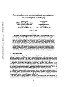
trimmings and then performing a set of non-overlapping backward (clockwise) trimmings. Thus each region is trimmed at most twice. The following is the actual algorithm we use. We walk around the polygon in the counter-clockwise direction applying the function ForwardTrim(B) (given below) to each vertex. This function removes some vertices and marks the ones that remain. We then walk around in the opposite direction applying the function BackwardTrim(B) to each vertex B that is not marked FAILED or STRONG by the rst stage. Finally, we remove all the vertices marked FAILED. At this point, all the vertices will be marked STRONG, meaning that they are 2�-strongly convex. We de ne the function ForwardTrim(B) to remove some of the successors (in the counter-clockwise direction) of vertex B. Let C be the original successor of B in H, and let C0 be the current successor of B after we have removed a number of vertices (see Figure 3). The function ForwardTrim(B) removes each successor of B from the polygon until one of the following occurs:
� � � �
IsStrong(B) is true; IsStrong(C0) is true; C0 is marked in some way (we have closed the loop); �(C0 ; BC) > 2�.
These conditions are checked in the given order, with the following actions taken: in the rst case, B is marked STRONG; in the middle two, B is marked FAILED; in the last, B is marked FTRIMMED.
Lemma 2 After the forward trimming stage, each vertex of H lies within 4� of the trimmed polygon. Proof. Figure 3 illustrates the case in which we halt the trimming at C0 because of the fourth termination condition. No matter what reason we halt the trimming, we know that the predecessor of C0 lies within 2� of lines BC and BC0 ; otherwise, we would have halted one step earlier. The portion of H from B to C0 lies inside the shaded region which lies within 4� of segment BC0 . As we walk around the polygon, we never remove BC0 . Thus we conclude that every point of the original polygon lies within 4� of some segment of the trimmed polygon. The function BackwardTrim(B) is de ned analogously to ForwardTrim. It can remove successors (in the clockwise direction) of B marked FAILED or FTRIMMED but not STRONG (because of the second termination condition). Naturally, the third termination condition refers to vertices marked in this stage, not the rst stage. The main di�erence is that if the fourth termination condition halts the trimming, then B is marked STRONG instead of FTRIMMED. We know from our discussion at the beginning of the section that B will in fact be 2�-strongly convex in this case. Lemma 2 implies that the rst trimmed polygon lies within 4� of the second trimmed polygon, and therefore, all points in H lie within 8� of the second trimmed polygon. Recall that the nal stage of the algorithm removes all the FAILED vertices at this point, leaving only STRONG vertices. The following lemma gives the error bound for this stage.
Lemma 3 After forward trimming and backward trimming, there is no string of more than three consecutive FAILED vertices. This implies that removing FAILED vertices adds at most another 4� to the error. Proof. After the forward trimming stage, each FAILED vertex is followed by a STRONG one (second termination condition) unless it is the last vertex marked (third termination condition), in which case it may be followed by a FAILED vertex followed by a STRONG one. Thus there may be at most one pair of consecutive FAILED vertices. Backward trimming can add at most one more FAILED vertex clockwise of each vertex marked FAILED by ForwardTrim (because, as before, each FAILED vertex must be followed by a STRONG vertex). At worst it creates one string of three FAILED vertices from the string of two created by the forward trimming.
6
If A, B, and C are consecutive vertices, and B is FAILED, then B is not STRONG, and therefore B lies within 2� of AC. Removing B only moves the polygon at most 2� farther from the original polygon. If we remove two or three consecutive FAILED vertices, the errors add, but not more than 4�. For two vertices this is obvious. For three, we rst remove the rst and third (no overlap) and then remove the second. Each stage of the algorithm moves the trimmed polygon at most 4� farther from the original convex hull H. The maximal distance from H to the nal �-strong polygon is 12�. Since all points in S lie inside H, they also satisfy this error bound. This proves the following theorem.
Theorem 4 Given the convex hull (of size h) of a set S of points, an �-strongly convex 12�-hull can be constructed in time O(h).
3 Arithmetic Models and Calculations Computing convex hulls, strong or otherwise, requires two geometric computations: the angle formed by two line segments, and the distance from a point to a line segment. The cost of calculating these quantities and the accuracy with which we can compute them depends on the input representation and the arithmetic model. We consider three types of representation for the vertex coordinates of the input: xed point, single precision oating point, and double precision oating point. We consider arithmetic operations on only the latter two types because xed point operations can be carried out using oating point arithmetic. The size and speci c properties of these representations depends on the computer, and so we present a general abstract model of computer arithmetic. The basic conclusion of this paper is that robust convex hull algorithms can construct convex hulls more e�ciently than an exact algorithm can construct them, unless the input representation is xed point and the arithmetic model is double precision oating point. Furthermore, for exact algorithms to have the advantage even in these most favorable circumstances, double precision addition and multiplication cannot cost more than three times as much as the single precision versions.
3.1 Arithmetic Model Fixed point representation is essentially integer representation with the implicit understanding that each number is multiplied by some xed power of two. Floating point representations contain an explicit exponent eld as well as mantissa. The value represented by a oating point number with mantissa m and exponent e is 2e m. The xed or integer representation has BI bits; the single precision oating point mantissa has BS bits; and the double has a BD -bit mantissa. For a typical computers such as a Vax or Sun or PC, BI is 16 or 32, BS is 21 and BD is 53. We make the reasonable assumption that BS < 2BI and BD > 2BS . In words, single precision is not twice as big as an integer, but double precision is at least twice as big as single precision. Mathematically, the consequence of single precision having BS bits is that every single precision operation has a relative error bound of 2?BS . For example,
j(a +BS b) ? (a + b)j � 2?BS ja + bj; where a +BS b refers to the sum of a and b computed using single precision arithmetic. The analogous bound holds for the other three operations. This broad assumption holds for all oating point representations. Particular oating point representations may have more speci c properties [6], but we do not exploit them here. For a given set of points in two dimensions, the diameter � of the set is de ned as usual: the maximum distance between a pair of points in the set. For geometric calculations on a set of points, absolute error is measured as a multiple of the rounding unit � = 2?BS �. This multiple is independent of precision and scale. 7
3.2 Calculating Angles An essential calculation in constructing convex hulls is to determine if two line segments AB and BC form a convex or concave angle. The robust convex hull algorithm requires the slightly more general operation of computing the angle formed by separate line segments AB and CD. Without loss of generality, assume that the two segments have positive slope and \point to the right": Ax < Bx , Ay < By , Cx < Dx , and Cy < Dy . De ne �(AB) to be the angle that line AB makes with the x-axis. De ne �(AB; CD) = �CD ? �AB to be the angle that line CD makes with line AB. The following exact arithmetic function determines if �(AB; CD) is greater than or equal to zero. PositiveAngleSign (AB, CD) if [(Bx ? Ax)(Dy ? Cy ) ? (By ? Ay )(Dx ? Cx) � 0] then return true else return false Actually calculating the angle �(AB; CD) requires taking a square root and arcsine. However, we can avoid these by computing the relative change in slope, tan �(CD) ? tan �(AB) ; � (AB; CD) = j tan �(CD)j + j tan �(AB)j
Dy ? Cy ? By ? Ay D = D x??CCx BBx ??AAx ; y y y + y D ? C B ? A x x x x (By ? Ay )(Dx ? Cx ) : = j((BBx??AAx)()(DDy??CCy))j ? + j(By ? Ay )(Dx ? Cx )j x x y y
Under the assumption that all segments have positive slope, we can leave out the absolute values. We can compute the relative change in slope using the third formula, or if we wish to avoid any divisions, the following function determines if the relative change in slope is greater than a particular value �. RelativeSlopeCompare (AB, CD, �) if [(Bx ? Ax)(Dy ? Cy ) ? (By ? Ay )(Dx ? Cx) > �((Bx ? Ax )(Dy ? Cy ) + (By ? Ay )(Dx ? Cx))] then return true else return false Exact convex hull algorithms use PositiveAngleSign, and the robust algorithms presented here use RelativeSlopeCompare. It might appear that RelativeSlopeCompare is more expensive to compute, but if one exploits common subexpressions, it only requires one extra addition and one extra multiplication to implement. Furthermore, as the following lemmas show, the actual cost of exact calculations may be much higher than their apparent cost.
Lemma 5 PositiveAngleSign can be computed exactly using double precision additions (or subtractions) and multiplications. The following table gives bounds on the number of operations required for various types of input. In the case of xed point inputs, four of the additions can be performed using integer operations.
Input Representation Additions Multiplications Fixed Point 5 2 Single Precision Floating Point 7 8 Double Precision Floating Point 71 72
Lemma 6 RelativeSlopeCompare can be computed approximately using 6 single precision oating point additions and 3 single precision oating point multiplications. The absolute accuracy is (3 + 6�) � 2?BS . In particular,
8
� if RelativeSlopeCompare(AB; CD; �) = true then � (AB; CD) � � ? (3 + 6�) � 2?BS ; � if RelativeSlopeCompare(AB; CD; �) = false then � (AB; CD) < � + (3 + 6�) � 2?BS . The error bound using double precision arithmetic is (3 + 6�) � 2?BD .
In practice, we only invoke RelativeSlopeCompare for small values of � (about 32 � 2?BS ). In this case, we can neglect the error term 6 � 2?BS �. For this reason, in the rest of the paper, the error bound will be simply 3 � 2?BS . As it will turn out, the robust convex hull algorithm makes two calls to RelativeSlopeCompare for every call to PositiveAngleSign made by an exact algorithm. However, by exploiting common subexpressions, the robust algorithm can be made to use only four single precision multiplications for every two double precision multiplications made by the exact algorithm. This is assuming that the exact algorithm is acting on integer inputs. In this case it is probably best to use the exact algorithm. However, if the inputs are single or double precision, the approximate algorithm has a clear advantage. Proof. (Lemma 5) In the case of xed point inputs, four subtractions can be carried out in xed point (integer) arithmetic without rounding. The remaining two multiplications and one subtraction can be carried out in double precision, and no roundo� error will occur|assuming that double precision can hold the square of an integer. In the case of single precision oating point inputs, the expression can be expanded in eight terms consisting of the product of two single precision oating point numbers. Each of these products can be performed in double precision, and there exists a way of summing the eight resulting double precision numbers in double precision so that the result is guaranteed to have the same sign as the exact answer.3 Finally, in the case of double precision oating point inputs, each input can be expressed as the sum of three single precision oating point numbers. Expanding as before results in 72 double precision terms to be summed. Proof. (Lemma 6) A relative error of 2?BS in the calculation of Bx ? Ax results in an absolute error of 2?BS (Bx ? Ax )(Dy ? Cy ) in the calculation of the expression, (Bx ? Ax )(Dy ? Cy ) ? (By ? Ay )(Dx ? Cx ): Similar bounds hold for the two multiplication and three of the other subtractions. The sum of these errors is bounded by, 3 � 2?BS ((Bx ? Ax )(Dy ? Cy ) + (By ? Ay )(Dx ? Cx )): The nal subtraction evaluated results in an absolute error bounded by, 2?BS j(Bx ? Ax )(Dy ? Cy ) ? (By ? Ay )(Dx ? Cx)j: This corresponds to a relative error of up to 2?BS in the calculation of the angle. Since this error is relative, we can treat it as if it occurs to the right hand side of the inequality. Using similarly reasoning, it can be shown that the absolute error in computing the expression,
�((Bx ? Ax )(Dy ? Cy ) + (By ? Ay )(Dx ? Cx )); is bounded by,
5 � 2?BS �((Bx ? Ax )(Dy ? Cy ) + (By ? Ay )(Dx ? Cx )); (one extra multiplication). The transfer of error from the right to the left changes the 5 to a 6. Together these error bounds imply the lemma.
3 Numbers with aligned least signi cant bits can be added without roundo� occurring. Otherwise, add numbers from smallest to largest.
9
3.3 A Note on Computing Angles In the rest of the paper, we will treat � (AB; CD) as if it were �(AB; CD), the actual angle between segments AB and CD. We can do this for two reasons. First, � (AB; CD) is always an overestimation of �(AB; CD). In particular, � (AB; CD) � sin �(AB; CD) � �(AB; CD); for all positively sloped line segments that \point to the right." For AB and CD nearly horizontal or vertical, � (AB; CD) is much larger than �(AB; CD). This means that an absolute error of 3 � 2?BS in the measurement of � corresponds to a much smaller error in the measurement of �. The second reason that we can replace � by � is that for xed AB, � (AB; CD) is a monotonic function of �(AB; CD). This implies the following lemma which we use in Section 4.2.
Lemma 7 If � (AB; BC); � (AB; CD) < �, then � (AB; BD) < �. Proof. This simply follows from the monotonicity of � and the fact that,
min(�(BC); �(CD)) � �(BD) � max(�(BC); �(CD)):
3.4 Geometric Distance The signed distance from a point C to a line AB can be computed by the formula, � AC = (Bx ? Ap x )(Cy ? Ay ) + (By ? Ay )(Cx ? Ax ) : �(C; AB) = ABjAB j (Bx ? Ax )2 + (By ? Ay )2 The distance function has positive sign when C lies to the left of AB as viewed from A looking at B. The following function determines if �(C; AB) is greater than a positive value �. The version which handles negative � is straightforward, and it involves the same number of arithmetic operations. DistanceCompare (AB, C, �) if [(Bx ? Ax)(Cy ? Ay ) ? (By ? Ay )(Cx ? Ax) � 0 and ((Bx ? Ax )(Cy ? Ay ) ? (By ? Ay )(Cx ? Ax ))2 � �2 ((Bx ? Ax )2 + (By ? Ay )2 )] then return true else return false DistanceCompare avoids division and square roots. Even for xed point inputs, computing this function exactly costs more than using approximate arithmetic. For double precision inputs, the approximate version is considerably cheaper, as it was for comparing angles.
Lemma 8 DistanceCompare can be computed approximately using single precision oating point operations. The absolute accuracy is 3 � 2?BS jABj + 6:5� � 2?BS . The error bound using double precision arithmetic is 3 � 2?BD jABj + 6:5� � 2?BD . Proof. (partial) The proof of this lemma is similar to that of Lemma 6. As with RelativeSlopeCompare, we will invoke this function for only very small values of �. Hence, we will use the error bound 3 � 2?BD jABj which is in turn bounded by 3� since jABj � �, the diameter of the set of input points.
10
H** H* H
Figure 4: Monotonic Sequence Containing Section of Convex Hull
4 Robust Convex Hull Algorithm In order to implement the algorithm of Section 2 using single (or double) precision oating point arithmetic, we apply Lemma 8. Replacing 2� by 2� + 3� wherever it appears assures that the rounded version will still generate an �-strongly convex polygon. However, instead of a 12�-hull, the output is a (12� + 18�)-hull.4 Unfortunately, rounded arithmetic does not allow us to construct the convex hull we need to get started. The rest of this section will show how to modify the standard Graham algorithm to generate a convex 36�-hull of a set S of n points in O(n log n) time. Using this instead of the convex hull results in a �-strongly convex (12� + 54�)-hull. The rst step is to extract four monotonic sequences of points from S which cover the vertices of the convex hull. For each sequence, the x and y coordinates are monotonic functions of index. To generate a sequence, we sort S by increasing x-coordinate and then examine the vertices in that order. Every time we encounter a vertex whose y-coordinate is less than or equal to the greatest y-coordinate we have seen so far, we throw it out. If several vertices have the same x-coordinate, we throw out all but the one with the largest y-coordinate. In Figure 4, vertex H is the head of the sequence and H* and H** are subsequent elements, where \*" is the successor operator. To generate the other three sequences we run the same algorithm on the original set S , but with the sense of the comparison in the x-direction or the y-direction or both switched. Figure 4 illustrates the four sequences. The increasing sequences are solid and the decreasing sequences are dotted. The next three sections will describe how to extract the vertices of a convex polygonal curve from each monotonic sequence. Putting the four parts together generates a convex 36�-hull. Generating the monotonic sequences costs O(n log n) (to sort the x-coordinates). Extracting the convex curves is O(n).
4.1 Extracting A Spine It can be shown that if we naively remove re ex vertices from a monotonic sequence, we may introduce error
n� because non-re ex vertices may appear to be re ex as a result of roundo� error. Instead, we rst create
a sequence of vertices and edges we call a spine which is a subsequence of a monotonic sequence. Removing re ex vertices from a spine introduces only O(�) error. This section gives the algorithm for creating a spine, 4 Each time we think we are removing 2� + 3�, we may actually be removing an extra 3�, hence an addition error of 6 � 3� = 18�.
11
E**
L
V0
E
V
E*
8 . 2 -P radians
Figure 5: Polygonal Curve of Vertebrae and Extenders (P = BS for Single Precision Floating Point) Section 4.2 proves that it is a 30�-hull. Section 4.3 shows that removing the re ex vertices from the spine adds only 6� more error. A spine is a sequence of edges of two types: vertebrae and extenders. These edges satisfy three conditions: 1. the rst edge is a vertebra, and each vertebra is followed by at most one extender; 2. each vertebra is rotated at least 18 � 2?BS radians clockwise with respect to the preceding vertebra; 3. each extender is rotated between ?6 � 2?BS radians and 24 � 2?BS radians clockwise with respect to the preceding vertebra, and it is rotated at most 6 � 2?BS radians clockwise with respect to the succeeding vertebra. Figure 5 depicts a spine. The dark edges are vertebrae, and the dotted edges are extenders. The vertices V and E and the edge E*E** are discussed in the following paragraph. The vertex V0 and the line L are part of the statement of Lemma 10 below. Intuitively, the angles of the vertebrae form an increasing sequence (using the de nition of the angle of an edge given in Section 3.2). An extender may be re ex with respect to one of its neighboring vertebrae, but only a little bit. Like the Graham algorithm for growing a convex hull, we \grow" a spine from left to right by removing vertices from a monotonic sequence. At any point in the computation, we have a partially constructed spine followed by unprocessed edges. Let VE be the rightmost vertebra, and let EE* be the extender that follows it. If no extender follows it, then E = E* (zero-length extender). Let E*E** be the next unprocessed edge. RelativeSlopeCompare(E*E**; VE; �) is true if the clockwise rotation of E*E** with respect to VE is greater than �, as calculated using rounded arithmetic. Recall that Section 3.2 describes how to compute RelativeSlopeCompare. Section 3.3 discusses the fact that RelativeSlopeCompare does not actually compute angles but that for the purposes of discussion and proof of error bound, one can assume it does. A. If RelativeSlopeCompare(E*E**; VE; 21 � 2?BS ) = true, make E*E** a vertebra. B. If not, merge E*E** with the extender EE*. That is, throw away E* if E* 6= E. Vertex E** changes its name to E*. C. If RelativeSlopeCompare(VE; EE*; 3 � 2?BS ) = true (newly created extender forms re ex angle with vertebra), throw away E also. Newly created edge VE* is added to list of unprocessed edges.
12
4.2 Proof of Algorithm We prove the correctness of the algorithm in two stages. First we prove that it satis es conditions 1, 2, and 3. Then we show that the generated spine is a 30�-hull.
Lemma 9 Each time rules A, B, and C are applied, the partially constructed spine satis es conditions 1, 2, and 3.
Proof. Most of the proof follows immediately from the fact that we can measure angles with accuracy plus or minus 3 � 2?BS (Lemma 6). The most di�cult part is showing that the new extender created by growth rule B satis es condition 3. Condition 1 is easy to check. Condition 2 is a consequence of rule A. An edge becomes a new vertebra only if its calculated rotation with respect to the previous is at least 21 � 2?BS greater. This implies that the actual angle is at least 18 � 2?BS greater. The 24 � 2?BS bound in in Condition 3 is a consequence of rule B. An edge is merged with the current extender if its rotation appears less than 21 � 2?BS . This implies that the actual angle is no more than 24 � 2?BS . If the extender satis es this bound before we merge the new edge, it will satisfy it afterwards. Rule C ensures that ?6 � 2?BS bound holds in condition 3. For if it did not, then the calculated angle of the extender with respect to the vertebra would be at least ?3 � 2?BS , and rule C would delete it. Finally, Rule A ensures that the 6 � 2?BS bound holds in condition 3. The calculated angle of the extender with respect to the preceding vertebra is at most 21 � 2?BS , and the calculated angle of the succeeding vertebra with respect to the preceding vertebra is at least 21 � 2?BS . Both these computations can be o� by 3 � 2?BS , and thus the total error is bounded by 6 � 2?BS .
Lemma 10 Let V0 be a vertex which is the left endpoint of a vertebra, and let L be the line through V0 rotated 6 � 2?BS radians counter-clockwise with respect to the vertebra. Every point of the spine to the right of V0 lies to the right of L (Figure 5). Proof. Condition 3 implies that the succeeding extender may be parallel to L at worst. Each subsequent vertebra is rotated at least 18 � 2?BS clockwise with respect to the vertebra of V0 , and each subsequent extender is rotated at least 12 � 2?BS .
Lemma 11 Suppose we run the spine algorithm and at time s, V0 is the left endpoint of a vertebra V0 Es, and at some later time t, it is the left endpoint of a di�erent vertebra V0 Et. Then V0 Et will be rotated counter-clockwise with respect to V0 Es. Proof. It su�ces to assume that when V0 Es was deleted, V0 Et was the next vertebra created. However, this means that V0 Et was created from an unprocessed edge generated by rule C. This edge is rotated counter-clockwise from V0 Es because V0 EsEt is a re ex angle.
Lemma 12 Let V0V0 * be any vertebra in the nal result. For all points P in S to the right of V0 , V0 P is rotated at most 6 � 2?BS counter-clockwise with respect to V0 V0 *. In other words, P lies to the right of L in Figure 5. Proof. Assume there is some P that violates this lemma. When we rst encounter P at time t, the point V will be the left endpoint of some vertebra, perhaps not the same as the one in the nal result. However, if it is not the same, it will be rotated clockwise with respect to the nal vertebra, by Lemma 11. Furthermore, the rightmost vertebra VE at time t will be rotated even more clockwise. On the other hand, V lies to the right of L (Lemma 10) and to the right of V0 . Therefore VP will be rotated counter-clockwise with respect to V0 P. As a consequence, angle EVP will be greater than 6 � 2?BS radians, and growth rule C will assure that E will be deleted. Ultimately, all the vertices between V0 and P will be deleted in the same fashion. This is a contradiction because we would then delete V0 * from the nal result.
13
P
E*
L E
< 40 . 2 -P radians
< 8 . 2 -P radians V Figure 6: Region Trimmed by Extract (P = BS for Single Precision Floating Point)
Lemma 13 No point lies farther than 30� outside the spine. Proof. It su�ces to prove this bound for all points P in the monotonic sequence. Let VE and EE* be the vertebra-extender pair such that P appears somewhere in the original monotonic sequence between V and E*. Lemma 12 implies P lies in a region depicted in Figure 6. Line L forms an angle of 6 � 2?BS radians with respect to VE, and EE* forms an angle of at most 24 � 2?BS radians in the other direction (condition 3). Therefore angle E*VP is bounded by 30 � 2?BS radians. The distance from P to the spine is bounded by �(P; VE*) < 30 � 2?BS jVE*j < 30 � 2?BS � � = 30�: This completes the proof that the spine is a 30�-hull.
4.3 Removing Re ex Angles The spine may still have some re ex angles. This section describes a simple post-processing stage which removes these angles without introducing much more error. If an extender might form a re ex angle with one of the neighboring vertebra (if the calculated angle is less than 3 � 2?BS ), we remove the appropriate endpoint. Because of the large angle (at least 18 � 2?BS ) between successive vertebra, we never remove both endpoints of an extender. Hence, removing potentially re ex angles trims o� another region of thickness at most 6� and alters the orientation of the vertebra by at most 6 � 2?BS radians. Since vertebra di�er in orientation by at least 18 � 2?BS radians before the nal trimming, they di�er by at least 6 � 2?BS radians afterward, and thus all angles are measurably convex. Total error is 36�. Removing the re ex vertices only requires linear time. Therefore we shown have the following.
Theorem 14 Using oating point arithmetic with P -bit mantissa and rounding unit � = 2?BS �, one can
construct a convex 36�-hull of a set of n points in O(n log n) time. To obtain B bits of accuracy, only (B + 6)-bit arithmetic is required.
If we cared to, we could replace 21 � 2?BS in rule A by a larger angle 21 � 2?BS + 2�=�. Then, in the post-processing stage, we would remove any angles whose calculated value is less than �=� + 3 � 2?BS . This 14
would ensure that all the angles5 are measurably greater than �=� at the cost of increasing the total error to 4� + 36�.
5 Conclusion Our approximate hull constructions have optimal complexity of O(n log n) and optimal error bounds of a constant times � plus a constant times �. As discussed in the introduction, the (n log n) cost of sorting the vertices by x-coordinate is xed and independent of the algorithm used to construct the hull thereafter. For the actual hull construction, our technique can achieve double precision accuracy on double precision inputs with less cost than the exact algorithm. Constructing the �-strongly convex (12� + 54�)-hull requires only a linear number of additional arithmetic operations. For any amount of input precision, our robust algorithm can perform this construction with less cost than the exact algorithm. An �-strongly convex polygon has the property that all angles are less than � ? �=� radians, where � is the diameter of the polygon. However, if that property is the only one we desire, than for any positive angle �, we can can construct a polygon whose angles are all less than � ? � which is a (4�� + 36�)-hull. Thus the constructed polygons have all the desirable properties outlined in the introduction. In the introduction, we made the claim that the ability to construct strongly convex objects should make it easier to construct the Minkowski sum of two polygonal regions, or their intersection, using approximate arithmetic. For both of these operations, there exist fast algorithms for convex polygons which do not work on general polygons. In the case of the Minkowski sum, the fast algorithm merges the two sets of edges so that the resulting set is ordered by angle. This algorithm would not work if the edges of one polygon attain the same angle multiple times, as may happen in a general polygon. The robust algorithm will not work if the edges appear (as a result of roundo� error) to attain the same angle multiple times. However, if the error in measuring angles is �, the input polygons will not appear to have parallel edges if all of its angles are less than � ? �. One fast way to intersect convex polygons is to look at them in the dual space in which each edge becomes a point and each vertex becomes a line. Again we merge the lists of points by angle and then compute the convex hull. In this case we might need the results of this paper twice: rst to assure proper merging by angle, second to compute the convex hull in the dual space. Robust Minkowski sums and polygon intersections are a subject for another paper, but it is clear that the ability to robustly construct strongly convex polygons is a prerequisite. Another claim made in the introduction is that strongly robust polygons make it possible to apply Euclidean transformations to a polygon. For example, suppose we wished to construct the intersection of two polygons: the rst one as it is, and the second after a rotation and translation. For a bounded number of translations, there will be some � such that an �-strongly convex polygon will remain convex after that number of translations. If we wish to use a robust intersection algorithm, we can use a slightly larger value of �. If we have to apply more transformations than we anticipated, we will still have to recompute the convex hull of the transformed polygon, but the use of strongly convex polygons eliminates the need to recompute the convex hull each time we perform a transformation. Our algorithm for constructing �-strongly convex polygons is practical. An empirical study shows that it generally introduces only � error, which is the lower bound, instead of the upper bound of 12�. Figures 7 and 8 show that output of the algorithm for � = 0:5 and � = 1, respectively, on a large convex polygon. One can see that the trimmed polygon lies only about � distant from the original convex hull. Currently we are implementing the robust version. We expect that the typical error will be much smaller than 54�. As we have seen, our techniques of spine construction and trimming are successful in two dimensions. The logical next step is to look for generalizations to higher dimensions. Similar results in three or more dimension would have a great practical impact on the cost of computing convex hulls and Voronoi diagrams of non-planar sets of points. 5 These are the angles. An external angle of � corresponds to an internal angle of � ? �. external
15
Strong Convex Hull with 9 Points Initial Convex Hull with 274 Points 80
y-axis
60
40
20
0 0
20
40
60
80
100
x-axis
Figure 7: �-Strongly Convex Polygon: � = 0:5 Strong Convex Hull with 6 Points Initial Convex Hull with 274 Points 80
y-axis
60
40
20
0 0
20
40
60
x-axis
Figure 8: �-Strongly Convex Polygon: � = 1 16
80
100
References [1] Steven Fortune. Stable Maintenance of Point-Set Triangulation in Two Dimensions. In 30th Annual Symposium on the Foundations of Computer Science, IEEE, October 1989. [2] Ronald Graham. An E�cient Algorithm for Determining the Convex Hull of a Finite Planar Set. Information Processing Letters, 1:132{133, 1972. [3] Leonidas Guibas, David Salesin, and Jorge Stol . Epsilon Geometry: Building Robust Algorithms from Imprecise Computations. In Proceedings of the Symposium on Computational Geometry, pages 208{217, ACM, July 1989. [4] Leonidas Guibas, David Salesin, and Jorge Stol . Constructing Strongly Convex Approximate Hulls with Inaccurate Primitives. In Proceedings of the SIGAL International Symposium on Algorithms, Tokyo, Japan, August 16-18, 1990. [5] Victor Milenkovic. Calculating approximate curve arrangements using rounded arithmetic. In Proceedings of the Symposium on Computational Geometry, ACM, pages 197{207, June 1989. [6] Victor Milenkovic. Double Precision Geometry: A General Technique for Calculating Line and Segment Intersections Using Rounded Arithmetic. In 30th Annual Symposium on the Foundations of Computer Science, IEEE, October 1989. [7] Victor J. Milenkovic. Veri able Implementations of Geometric Algorithms using Finite Precision Arithmetic. Ph.D. Thesis, Carnegie-Mellon, 1988. Technical Report CMU-CS-88-168, School of Computer Science, Carnegie Mellon University, Pittsburgh, PA 15213, July 1988. [8] Kokichi Sugihara and Masao Iri. Construction of the Voronoi Diagram for One Million Generators in Single-Precision Arithmetic Presented at First Canadian Conference on Computational Geometry, August 21-25, 1989, Montreal, Canada. Available as preprint, Department of Mathematical Engineering and Information Physics, Faculty of Engineering, University of Tokyo, 7-3-1 Hongo, Bunkyo-ku, Tokyo 113, Japan.
17