Apr 5, 2006 - such operators as elements of the full tensor algebra T(g) of the Lie algebra g of KC. .... Vλ, such that t.x = 2Ïiλ(t).x for x â Vλ,t â t and λ â tâ is the highest weight. A vector .... relation AB â BA â [A, B] for A, B â g is in the kernel of every ̺* . Even if ... The resulting classical limit cl is physically well-behaving,.
arXiv:math-ph/0604010v1 5 Apr 2006
Constructing the classical limit for quantum systems on compact semisimple Lie algebras Ingolf Sch¨afer Fakult¨ at f¨ ur Mathematik, Ruhr-Universit¨at Bochum, D-44780 Bochum, Germany Marek Ku´s Centrum Fizyki Teoretycznej PAN, Al. Lotnik´ ow 32/42, 02-668 Warszawa, Poland Abstract We give a general construction for the classical limit of a quantum system defined in terms of generators of an arbitrary compact semisimple Lie algebra, generalizing known results for the su2 and su3 cases. The classical limit depends on the physical problem in question and is determined by the sequence of representations by which it is reached. Only in the simplest cases it is unique. We present explicit formulae useful in determining the classical limit in all important cases.
1
Introduction
Although a natural setting for a quantum mechanical system is the infinite-dimensional Hilbert space, there are many circumstances when the complex projective space PN suffices to describe quantum dynamics. The most commonly known situations concern various spin systems when spatial and spin degrees of freedom are sufficiently decoupled and we are interested only in the evolution of the latter. In such cases, however, the notion of the classical limit rarely makes sense, or, at least, is not immediately obvious. There are, however, quantum systems living in finite-dimensional Hilbert spaces (or, more correctly, their projectivisations), for which a construction of a classical limit is sensible and conceptually simple. Let us consider a system of N atoms interacting resonantly with electromagnetic radiation. Resonance conditions usually ensure that only a finite number M of energy levels of each atom is effectively excited by the interactions. The operators skl = |kihl| describing transitions from the level |li to the level |ki of a single atom, after multiplying by the imaginary unit i, span the defining representation of glM (C). For a system of N atoms confined to a small volume - so small that P theyµfeel the same field amplitude - it is convenient to introduce collective operators Skl = N µ=1 skl where µ skl acts as skl on the levels of the µ-th atom and as the identity on the rest. If the atoms do not interact, the dynamics of the system can be described only in terms of Skl , k, l = 1, . . . , M 1
and their couplings to the electromagnetic field. It is clear that, again up to the multiplication by i, Skl , obeying the same commutation relations as skl , i.e. [Skl , Smn ] = δml Skn − δkn Sml , span a (in general reducible) M N -dimensional representation of glM (C). In a typical situation the number of atoms is conserved and we can restrict our attention to slM . This is due to the fact ˆ = S11 + S22 + · · · + SM M , counting the number of atoms, is a constant of that the operator N motion. The above described example can be used to illustrate the main topic of the present paper - a kind of classical limit for a quantum system appearing when the number of its constituents (in our case atoms) is very large and we are interested in such quantities like e.g. energy or polarization per one atom. Such a situation in which we formally put N → ∞ is common in constructing semiclassical theory of lasers (for a particular example where such an approach to the classical limit was applied to the so called superradiant laser in which the active medium consisted of three-level atoms see [See96]). In the limit we expect quantum operators constructed from the generators Skl , after scaling by the number of atoms, to be mapped into functions defined on a classical phase space. By the classical phase space we understand an appropriate symplectic manifold determined by the problem in question. Moreover, to have an unambiguous connection between quantum and classical dynamics, we demand the Dirac connection between commutators and Poisson brackets: the classical limit of the commutator of two operators should be proportional to the Poisson bracket of the corresponding classical limits of the operators involved. Such a connection assures that the classical dynamics will be obtained by applying classical limit procedure to the quantum (Heisenberg) dynamics. In [GK98] a detailed analysis of the problem in the case K = 3 was presented. The classical limit was constructed with the help of coherent states for the group SU3 . (The complexification of SU3 , i.e. SL3 (C) has, as its Lie algebra sl3 , generators of which appeared above as relevant operators in the case of systems of three-level atoms). The classical limit was obtained by taking appropriately scaled expectation values of quantum operators in the coherent states and going to infinity with the dimension of representation. On the manifold of the coherent states there exists a natural symplectic structure which, in the classical limit, gives the classical canonical structure. In the above construction we still have a freedom to choose the way we go to infinity with the dimension of representation. Obviously the actual way must be decided upon the actual physical problem in question. Thus, for example in the above mentioned case of multilevel atoms, we may consider a situation when initially the system is prepared in the ground state, independently on the number of atoms involved. Such a choice determines for each number of atoms a particular irreducible representation. Increasing now the number of atoms we approach the classical limit via a particular sequence of irreducible representations. It was shown in [GHK00] that the choice of the way to the classical limit may have measurable consequences. In the considered case of many three level systems there are at least two natural ways in which the classical classical limit is achieved. The integrability properties of the system, as well as statistical properties of spectra, distinguishing chaotic and integrable system on the quantum level, were shown to depend on the way chosen, which makes the whole problem interesting and worth reconsidering in the more general setting (see also [See96] where the non-hamiltonian classical dynamics appropriate for the superradiant laser is analyzed). The present paper generalizes the above ideas to an arbitrary compact semisimple Lie group K. We do not use explicitly the concept of coherent states - a crucial element of the papers [GK98] and [GHK00], choosing a more straightforward way of identifying classical phase space 2
with an appropriate orbit of the group and obtaining the classical function with the help of the moment map. The whole construction is, however, completely equivalent to the one using coherent states. The crucial point consists of extending the straightforward procedure of obtaining classical limit for generators of the Lie algebra of K C to operators which are polynomials in the generators, as these appear in a natural way in nontrivial quantum systems. We chose to treat such operators as elements of the full tensor algebra T (g) of the Lie algebra g of K C . We show how they are represented as differential operators, obtainable from the differential operators for the generators, and how to perform the classical limit of them. We give formulae useful for an arbitrary compact semisimple group which allow the explicit calculation of classical limits for different sequences of representations. The most important application we had in mind is the above outlined generalization from three-level systems to ones with M levels. In this case K = SUM but, obviously, the generality of the construction gives a possibility to analyze systems with an arbitrary compact, semisimple group of symmetries. In a forthcoming paper we shall apply the construction to the above mentioned problem of spectral statistics of quantum evolution operators for classically integrable and non-integrable systems. The two following sections of the paper give necessary definitions, conventions and short description of properties of the momentum map for a compact group action on a symplectic manifold (Section 2) and some basic facts from the theory of representations for compact groups (Section 3. Sections 4 and 5 give a description of what is meant by a classical limit. The main results are contained in Section 6, where we give the formulae for calculating classical limit for an arbitrary Lie group, generalizing results obtained in [GK98]. A detailed proof of an important theorem concerning the factorization of the norm function on the orbits using methods of complex algebraic geometry, is given in the Appendix.
2
The momentum map
We start this section with the definition of momentum maps which will be used in the sequel to construct the classical limit by representation theoretic methods. In the simplest example of the system of free particles in 3 the momentum map assigns to each particle with a generalized momentum p at a point q in configuration space the negative of its momentum, i.e. −p, providing thus a map defined on the phase space. We shall see in the sequel that its codomain is more interesting. Since it is a good convention, let us call this map µ. The configuration phase space of the free particles system has translational symmetry, so 3 we have a natural action of the additive group of real 3-tuples, i.e. , by translation in configuration space. The ordinary momentum of a particle is a point in the tangent bundle, i.e. a tangent vector. Now we can view such a tangent vector as an infinitesimal generator of the group 3 , i.e. an element of the abelian Lie algebra 3 . Since generalized momenta are cotangent vectors, the momentum map µ can be thought of as a map
R
R
R
R
µ : phase space → dual of Lie algebra of
R3 .
Let us discuss the abstract definition of momentum map first. We start with a phase space (M, ω) being a smooth manifold M with a symplectic form ω. A Hamiltonian vector field ξH 3
on M is by definition a vector field which is induced by a smooth function H, sometimes called the Hamiltonian function, in such a way that the contraction of the form ω with ξH is the differential of H: iξH ω = dH. (1) Now let us consider a connected Lie group G of symmetries acting on M G × M → M,
(g, x) 7→ g.x
(2)
from the left. In order to be a group of symmetries, G has to act via canonical transformations or symplectic diffeomorphisms, i.e. for every g ∈ G: g ∗ω = ω,
(3)
where g ∗ denotes the pullback by the group action (2). In short words it simply means that the symplectic structure on M is invariant with respect to the action of G. What happens to the Lie algebra g of G here? Every ξ ∈ g induces a flow via exp(ξt), which is the flow of some vector field r(ξ) on M. The formula for r(ξ) applied to a smooth function f ∈ C ∞ (M) reads d (4) r(ξ)(f )(x) = f (exp(−ξt).x), dt t=0
which makes r a map r : g → Vect(M), where Vect(M) denotes the set of smooth vector fields on M. We adopted here the sign convention which is natural for the left action, otherwise we could choose to act on M from the right and dispose the minus sign here. Being a connected Lie group of symmetries g ∗ ω = ω for all g ∈ G
(5)
Lr(ξ) ω = 0 for all ξ ∈ g,
(6)
is equivalent to where, as customary, we denote by LX the Lie derivative along X. By Cartan’s formula we see that Lr(ξ) ω = d(ir(ξ) ω) + ir(ξ) dω and dω = 0, because ω as a symplectic form is closed by definition. So, Lr(ξ) ω = d(ir(ξ) ω) = 0 means that - at least locally - for every ξ there exists a function µξ , such that by Poincar´e Lemma dµξ = ir(ξ) ω.
(7)
Let us take a closer look at the situation, pretending everything is defined globally. For every ξ we have a map µξ : M → , (8)
R
so we get, by choosing a µξ for each ξ, a map µ : M → g∗ ,
x 7→ µ(·) (x),
where g∗ denotes the space dual to g.
4
(9)
One might wonder why µξ should be linear in ξ, but since dµξ = ir(ξ) ω is a linear condition, it is always possible to choose µξ in such a way. The choice is still a non-unique one here, because we can add any linear form α ∈ g∗ to µξ , i.e. µξ + α(ξ)
(10)
is also a Hamiltonian function to the vector field r(ξ). To reduce this non-uniqueness and at the same time make a connection to the group action, µ should be equivariant with respect to the coadjoint action on g∗ g.µ(x) = µ(g.x),
(11)
g.α(η) = α(Ad(g −1 ).η) for all α ∈ g∗ , η ∈ g.
(12)
where the coadjoint action is given by
Thus, let us formulate the following definition Definition 1 (momentum map) Let (M, ω) be a symplectic manifold with a Lie group action G × M → M by symplectic diffeomorphisms. A momentum map is a smooth map µ : M → g∗ , which is equivariant and satisfies dµξ = ir(ξ) ω for all ξ ∈ g.
(13)
By a straightforward calculation using the flow exp(ξt) one can immediately prove that the equivariance property of µ is equivalent to µξ being a Lie algebra homomorphism, i.e. µ[ξ1 ,ξ2 ] = {µξ1 , µξ2 }.
(14)
We proceed to the next section, in which we will give an explicit formula for the momentum map in our case.
3
A slice of representation theory for compact groups
Since our quantum mechanical systems are given by irreducible representation spaces of compact Lie groups, we should try to understand, at least roughly, how the representation theory works. Details can be found in [BtD85]. Let K be a compact connected Lie group. Since later it will appear to be necessary, let us assume from the beginning that K is semisimple. By the famous theorem of Peter and Weyl [PW27], we can think of K as a matrix group, more precisely K is isomorphic to a subgroup of some unitary group Un . The representation theory for K relies heavily on the existence of maximal tori, i.e. maximal, connected, abelian subgroups of K. So from now on, we consider K as a group of matrices with a fixed maximal torus T . We shall denote the Lie algebra of T by t and the Lie algebra of K by k.
5
Assume we have an irreducible, unitary representation1 ̺ of K on some finite-dimensional Hilbert space V . Certainly we can split V up into irreducible subspaces with respect to the T representation: M V = Vα and ̺ = ⊕α ̺α (15) α
The Vα are necessarily one-dimensional, because T is abelian. So T acts on these one-dimensional subspaces by multiplication with complex numbers of norm one. These representations are called the exponentiated weights of ̺ and are given by group homomorphisms ̺α : T → S 1 . If we take the differential, we get a Lie algebra morphism de ̺α : t → i . A good convention is 1 to scale de ̺α a bit differently and consider the maps χα = 2πi de ̺α : t → . These maps can ∗ be viewed as elements in the dual of the Lie algebra t of t and we call them the weights of the representation. To summarize, every irreducible unitary representation ̺ of K gives a sequence of points (infinitesimal weights) in t∗ . Since we do not want to go through all the details, let us just say that depending on some choice of ordering, we get a convex cone in t∗ , usually called the Weyl chamber, and that we can identify every irreducible, unitary representation by the so called highest weight2 in this Weyl chamber in t∗ , relatively to the chosen ordering. This fact is called the theorem of the highest weight and is due to Hermann Weyl. The set of the highest weights gives therefore a complete system of all irreducible representations up to equivalence. Moreover, there is a natural algebraic structure on the set of highest weights (namely it is an additive submonoid of the additive group t∗ generated by a finite number of so-called fundamental weights) - every highest weight has a unique representation as a linear combination X λ= λi fi , (16)
R
R
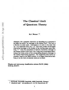
with generators fi and natural numbers λi . (cf. [BtD85] chap. VI and [Kna02] Theorem 5.5) For illustration consider the following picture of the highest weights of SU3 written in the coordinates (λ1 , λ2 ): Now we want to connect this to the momentum maps discussed earlier. To this end we embed t∗ into k∗ (the dual of k), with respect to the Killing form on k. More formally, we identify k with k∗ and have the inclusion of t∗ , if we extend every λ : t → to k = t ⊕ t⊥ by 0 on t⊥ . Using this identification, we can talk about K-orbits through λ ∈ t∗ . In particular we look at the coadjoint orbits through the highest weights. It is a well-known fact that the highest weight of a representation has multiplicity one, i.e. there is only a one-dimensional subspace Vλ , such that t.x = 2πiλ(t).x for x ∈ Vλ , t ∈ t and λ ∈ t∗ is the highest weight. A vector vmax 6= 0 in Vλ is called a maximal weight vector. Here we encounter the basic fact:
R
Theorem 1 Let ̺ : K → U(Vλ ) be an irreducible, unitary representation with the highe ̺(ξ).xi est weight λ, then we have a momentum map µ : (Vλ ) → k∗ , µξ ([x]) = −2i hx,dhx,xi and
P
1
In this article we consider only continuous representations, so we drop the adjective ‘continuous’ in the following whenever it applies to a representation. 2 In the literature there is normally a distinction between the weights (sometimes called real weights) and the points in t∗ , which are called (analytic) integral forms. This is reasonable for a complete treatment of the matter, but not necessary in this paper.
6
Figure 1: The highest weights of SU3 written in the coordinates (λ1 , λ2 ) µ([vmax ]) = λ. Moreover µ is a symplectic diffeomorphism between K.[vmax ] with the natural symplectic form and K.λ with the Kostant-Kirillov form (which is the natural symplectic structure on it). Proof The proof that µ is a momentum map can be found in [Huc91] chapter VI.7. The proof that µ([vmax ]) = λ, as well as of the rest of the statement, is given in chapter V (Theorem 7.2) of the same reference. �
P
The natural symplectic form of the (Vλ) is the one induced by the Fubini-Study metric, i.e. which is the imaginary part of the hermitian metric in Vλ given by i ¯ ·i, ω = ∂ ∂logh·, 2
(17)
P
pushed down to (Vλ ). A detailed description of Kostant-Kirillov form it is not important for the rest of the paper. We are more interested in restating the theorem in the following way: To every irreducible unitary representation we find a symplectic manifold M (the orbit K.[vmax ]) and a map µ ˜:k→ ∞ ξ C (M), ξ 7→ µ , which is a Lie algebra homomorphism, i.e. µ ˜([ξ, η]) = µ[ξ,η] = {µξ , µη }.
(18)
This is almost a quantization procedure.
4
The classical limit (simple case)
We now have a connection between some skew-selfadjoint operators in the image of de ̺λ and classical functions on some symplectic manifold. We would like, however, to have such a construction for self-adjoint operators appearing in a natural way as observables in quantum mechanics. Clearly, multiplying by i makes a skew-selfadjoint operator selfadjoint and vice versa. So let us consider the operators ξ = iA and η = iB. We get [ξ, η] = −[A, B] 7
(19)
and µξ = µiA .
(20)
cl : ik → C ∞ (M)
(21)
hx, Axi 1 . cl(A)(x) = µiA (x) = 2 hx, xi
(22)
We define our classical limit by
Thus we get the relation
1 cl(i[A, B]) = {cl(A), cl(B)}, (23) 2 which is, modulo the constant ~, the well known Dirac quantization scheme we wanted to have as explained in the Introduction.
5
The classical limit (general case)
Our classical limit has a major drawback. It is only defined for those self-adjoint operators which are in the image of the representation de ̺ multiplied by i. We would like to find a classical limit for the system, starting with a fixed representation ̺ on V and some arbitrary self-adjoint operator on V . Every continuous, irreducible, unitary representation ̺ of K gives a holomorphic representation of the complexification G = K C , which we call ̺ as well. By taking the derivative we get a representation L ̺∗ = de ̺ : g → End(V ). This has a unique extension to the full tensor algebra T (g) = n∈N g⊗n of g, by multiplying the images of generators in End(V ). The famous lemma of Burnside says that every operator in End(V ) is in the image of this representation on V , cf. [Far01]. This is good and bad in some ways. Good, because we may find a way to generalize our classic limit by algebraic methods, but bad because the procedure is not unique at all. The non-uniqueness results from the fact that the ideal generated by the relation AB − BA − [A, B] for A, B ∈ g is in the kernel of every ̺∗ . Even if we divided by this ideal, the resulting algebra U(g), called the universal enveloping algebra of g, would be infinite dimensional, so we would have a far greater kernel. To illustrate this consider for example the image of a nilpotent element α in g. In every representation it is mapped to a nilpotent operator. So let A be the matrix representing α in some suitable basis for a given representation, such that A is a matrix with zero on and below the diagonal. Then we will find some n ∈ , such that An = 0. This means αn is in the kernel of this representation. So, we can add αn to any operator in T (g), without changing the image of the representation of this operator. To overcome this, we need a notion of hermiticity on T (g) and define everything for these abstract operators independently of the chosen representation.
N
Definition 2 Let k be the Lie algebra of a compact, simple Lie group and g = k ⊕ ik be its complexification. We define the formal adjoint operation † : T (g) → T (g) by 1. (c · 1)† = c¯ · 1
8
2. ξ † = −ξ for every ξ ∈ k 3. ξ † = ξ for every ξ ∈ ik 4. (ξ1 ⊗ . . . ⊗ ξn )† = ξn† ⊗ . . . ⊗ ξ1† and and extend this definition to T (g) by linearity with respect to We call an element α ∈ U(g) abstractly selfadjoint, if α† = α.
R.
Remark 1 Note that the formal adjoint is not complex linear, because it contains the complex conjugation on the scalars in point 1. By the very definition an abstractly selfadjoint element is mapped to a selfadjoint operator by the extended derivative ̺∗ of every irreducible unitary representation ̺ : K → U(V ). To overcome this we start with a general, abstractly selfadjoint element ξH in T (g), which we call the abstract Hamiltonian of the system. Let us choose some basis ξ1 , . . . , ξk of g. We can decompose ξH uniquely into homogeneous terms consisting of sums of “monomials” ξα1 ⊗ . . . ⊗ ξαp for some indices αj ∈ {1, . . . , n}. We will extend the momentum map µ to these “monomials” simply by setting µξα1 ⊗...⊗ξαp = µξα1 · . . . · µξαp ,
(24)
where we have already extended the definition of µ to g by complexification, that is µξ ([x]) = −2i
hx, ̺∗ (ξ).xi hx, xi
for ξ ∈ g, x ∈ V.
(25)
We extend µ by linearity to T (g). The resulting classical limit cl is physically well-behaving, because if we take only unit vectors in Vλ , than cl(ξi ξj )(x) = cl(ξi)(x) cl(ξj )(x) = hx, ξi .xihx, ξj .xi,
(26)
which means that the expectation value of the operator ξiξj is given by the product of the expectation values ξi and ξj , i.e. in the classical limit ξi and ξj are stochastically independent operators. This is pretty unspectacular, because it was just defined to be this way, and we would really like so see this definition in the light of some limiting process, sending ~ → 0. A proposal how to do this is given in one case by direct calculation in [GK98], which we will discuss in the next chapter in general. The reader may wonder why we do not choose the universal enveloping algebra U(g) as starting point. For this consider ξ, ξ1, ξ2 ∈ g, such that 0 6= ξ = [ξ1 , ξ2 ]. In the universal enveloping algebra we have [ξ1 , ξ2] = ξ1 ξ2 − ξ2 ξ1 . The classical limit of the right hand side would be necessarily 0, because multiplication of functions is commutative, but the left hand side is just the classical limit of ξ, which is not 0. Therefore we cannot take U(g) as the basic algebra of our construction.
9
6
Realizing the classical limit as a mathematical limit process
So far we have a generalized classical limit defined on “monomials” cl(ξα1 ⊗ . . . ⊗ ξαp ) = cl(ξα1 ) · . . . · cl(ξαp )
(27)
and extended by linearity. We want to realize this limit by a limiting process, i.e. to have some sequence of C ∞ -functions converging uniformly on compact sets to the classical limit of the “monomial”. Our basic idea is that we should go to infinity along lines through the Weyl chamber by which we mean the following. Assume we start in a fixed point λ in the Weyl chamber, which is the highest weight of some irreducible, unitary representation ̺. Let us consider the discrete line n · λ in t∗ for n ∈ . It is again a standard fact - a corollary of the highest weight theorem - that each nλ is a highest weight of an irreducible, unitary representation ̺n : K → U(Vn ), such that for n 6= 0 all orbits K.(nλ) are diffeomorphic to each other. Moreover the isotropy subgroup is the same for every (nλ) and the diffeomorphisms are given by scalar multiplications. The dimension of the irreducible representation is given by (cf. [Kir04])
N
vol(K.(nλ + ρ˜)) = dim Vn ,
(28)
where ρ˜ is a known fixed vector in the Weyl chamber and vol denotes the volume taken with respect to the Killing metric. We need a little more details about the structure of g now. Let us consider the adjoint representation of G on g. We can surely decompose it into the one-dimensional irreducible representations of T . This leads to points in t∗ as described in section 3. They are in general called the weights of the representation, but since the adjoint representation is so fundamental, its weights have a special name - they are called the roots of the G. For every root α we find a one dimensional subspace of g called the root space to α and denoted by gα . The before mentioned ordering on t∗ gives a notion of positivity on the set of roots, i.e. we can decompose g in the following way g = u− ⊕ tC ⊕ u− ,
(29)
P P where u+ = α positive gα and u− = α negative gα are Lie algebras. In a good ordering of weights we can think of the matrices in u− (u+ ) as lower (upper) triangular matrices with zero diagonal and tC as diagonal matrices. The group U− = exp(u− ) is biholomorphic to n , because exp is a diffeomorphism here. Analogously, we define U+ = exp(u+ ). For the moment it is enough to state that we have a decomposition of the Lie algebra g which gives a decomposition of the group G outside a Zariski3 -closed set, such that
C
G∼ = closure of U− T C U+ . Moreover U+ ⊂ StabG (vmax ) (the stabilizer of vmax ) and T .vmax ⊂ on vmax and T C acts on it by scalar multiplication. 3
(30)
C∗ ·vmax, ie. U+ acts trivially
Readers not familiar with the Zariski topology may read this as closed set of lower dimension than the surrounding space.
10
It is a general fact [Huc91], that the orbit of U− through vmax in ̺λ is isomorphic to K.[vmax ]\A ⊂ (Vλ ), where A is a Zariski-closed set in K.[vmax ]. This leads to a chart of K.[vmax ] given by the greatest subgroup Umax of U− acting freely on U− .vmax . In the generic case, that is, if the highest weight is in the interior of the Weyl chamber, this group is U− itself. Otherwise we will have smaller unipotent groups. The main step is to view the original classical limit cl as composition, cl = r ◦ s, of two maps d 1 (31) r : ik → Vect(Vλ ), ξ 7→ − Xξ , with (Xξ f )(x) = f (exp(−ξt).x) 2 dt t=0
P
and
s : Vect(Vλ ) → C ∞ (Vλ \{0}), X 7→
1 (XNλ ), Nλ
(32)
where Nλ (x) = kxk2 is the norm function squared. Note, that we have intentionally changed our view point from (Vλ ) to Vλ . This is a crucial step. What we will do now is not possible in (Vλ ), or in physics language with normalized coherent states, we will have to use nonnormalized coherent states. The reasons for this step will be discussed after a short calculation. Let us thus apply the vector field r(ξ) to Nλ first. We have to calculate d (33) (Xξ Nλ )(x) = Nλ (exp(−ξt).x). dt t=0
P
P
Suppose that x is in the Umax -orbit through vmax . Thus, there exists u ∈ Umax , such that x = u.vmax .
(34)
Now we can decompose exp(−tξ)u as exp(−ξt)u = u− (t)l(t)u+ (t) for almost all4 t, such that u− (t) ∈ U− , l(t) ∈ T C and u+ (t) ∈ U+ . Using the chain rule and the self-adjointness of ξ we obtain d d (Xξ Nλ )(x) = 2hx, exp(−ξt).xi = 2hx, u− (t)l(t)u+ (t).vmax i. (35) dt t=0 dt t=0
Since u+ (t) ∈ U+ ⊂ StabG (vmax ), we have
d (Xξ Nλ )(x) = 2hx, u− (t)l(t).vmax i dt t=0
(36)
According to the product rule we get
d ˙ (Xξ Nλ )(x) = 2l(0)hx, xi + 2hx, u− (t).vmax i, dt t=0
(37)
where we used the fact that the l(t) ∈ T C acts diagonally. So, at last, we see that every vector field in the image of r when applied to Nλ acts like a first order differential operator, consisting 4 Such a decomposition is not possible for all elements of G, but on a dense, open set. This is enough for our purpose, because we can certainly decompose for t = 0 and then in a small neighborhood.
11
˙ of some multiplication operator l(0) and some vector field tangential to the Umax -orbit. The above procedure thus gives a map r˜ : ik → Diff(Umax .vmax ).
(38)
We extend r˜ to T (g) in the obvious manner, i.e. r˜(α1 ⊗ . . . ⊗ αp ) = r˜(α1 ) ◦ . . . ◦ r˜(αp ) for α1 , . . . , αp ∈ g
(39)
r˜ : T (g) → Diff(Umax .vmax ).
(40)
and get
C
1 r˜(α)(Nλ ) Nλ
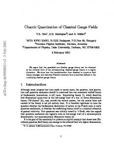
We can now define a map l : T (g) → C ∞ (Umax .vmax , ), α 7→ and by explicit calculation we see that l(αj ) = cl(αj ). Let us take some time to discuss more abstractly what we have done. We started with a vector field which is tangential to the G-orbit through vmax . In the result we get a first order differential operator, which has a vector field part tangential to the Umax -orbit, plus some multiplication part. This is very much like in the construction of connections on line bundles. Indeed, we have a line bundle here. To be more precise, it is only a ∗ -bundle. We start with the K-orbit through vmax . Since the G-orbit and the K-orbit through [vmax ] agree in (V ), we know that we only get points on the complex lines without 0 through the K-orbit.
C
P
Figure 2: The Umax -orbit as a section As Figure 2 indicates, the Umax -orbit is a non-trivial section in this line bundle outside a closed set of lower dimension and the multiplication part of our decomposition is just multiplication in the fibres. We see now, why this construction is not possible in (V ). There is no such line bundle, we have factored it out already. Let us try to give yet another description of what happened. The K-orbit is the set of normalized coherent states, while the Umax -orbit is the set of non-normalized coherent states. If we consider some motion in the Umax -orbit, we may project it to the K-orbit, but we will loose then the information encoded in the norm of the coherent state, i.e. the information which is the source of the multiplication part. This line bundle will be of great importance later, when it comes to the proof of the following theorem about the norm square Nλ : P Theorem 2 Let λ = ri=1 λi fi the decomposition of λ into fundamental weights, then we have the following factorization of Nλ on the U− -orbit
P
Nλ (x.vmax ) = c · N1 (x.vmax )λ1 · . . . · Nr (x.vmax )λr , 12
(41)
where c is a real constant and N1 , . . . , Nr are the squared norms of the fundamental, unitary representations corresponding to the fundamental weights f1 , . . . , fr . The proof of this theorem requires some methods of complex analysis and complex algebraic geometry, which are maybe not so commonly known and can be found in the Appendix. P Theorem 3 Assume that λ = i λi fi is given, such that at least one λi > p for a fixed positive natural number p. Let α = ξα1 ⊗ . . . ⊗ ξαp be a “monomial” element of degree p in the generators ξi of g, then l(α) is a polynomial of degree p in the λi ’s with coefficients in C ∞ (Umax .vmax , ). (Recall that the fi ’s were a basis of the discrete cone in the Weyl chamber.) Moreover the homogeneous part of degree p of l(α) is up to a real, multiplicative constant the product cl(ξα1 ) · . . . · cl(ξαp ). By a suitable choice of unitary metric this constant can be made equal to one.
C
Proof The r˜(ξαi ) involve only first order partial differentiations, hence the summands in the expanded derivative of Nλ = N1λ1 · . . . · Nrλr , after dividing by Nλ , are polynomials in λ of degree at most p and there will be at least one summand of degree p. Otherwise one of the ξαi is just the multiplication by a constant, what is not the case, or the partial derivatives would lower every exponent λi to 0, what is not possible since at least one λi is larger than p. Let us consider the case p = 1 first. In this case there will be no constant term, since l(ξi ) = N1λ r(ξi)(Nλ ) by the construction above. Now, r(ξi ) is a vector field and contains no multiplication term, so we have just partial derivatives turning Nλ into a homogenous polynomial of degree one after dividing by Nλ . For p > 2 we use the product rule of differentiation. We give the proof here only for p=2. The rest is an exercise in systematic bookkeeping P ∂ of indices. Let ξa and ξb be basis elements chosen from (ξ1 , . . . , ξn ). We have r˜(ξa ) = ai ∂zi + b for some ai and b (and some coordinate system {zi } on Umax .vmax ), and we can calculate l(ξa ⊗ ξb ): 1 1 r˜(ξa ) ◦ r˜(ξb )(Nλ ) = r˜(ξa )(Nλ · l(ξb )) Nλ N X ∂ 1 (b · Nλ · l(ξb ) + ai (Nλ · l(ξb )) = Nλ ∂zi � � X X ∂ 1 ∂ = l(ξb ) · b · Nλ + ai (Nλ ) + ai (l(ξb )) Nλ ∂zi ∂zi X ∂ (l(ξb )). = l(ξb ) · l(ξa ) + ai ∂zi
l(ξa ⊗ ξb ) =
(42)
The first summand is clearly a homogenous polynomial of degree two in the λi ’s, while the second lower the degree, because l(ξb ) is a polynomial of degree one, and taking the derivative on a polynomial lowers the degree by one. � The formula (42) should be compared with the explicit relations (3.15) for the SU3 case obtained in [GK98]. With this theorem we can give an explicit construction of the classical limit in terms of the map l. For the moment we have to refine our notation and use lλ instead of l to exhibit explicitly the dependence on the highest weight λ. Let us now fix a given irreducible representation with 13
the highest weight λ, an abstract Hamiltonian ξH ∈ PT (g) and a basis ξi of g. Split ξH into sums of monomial elements αi = ξi1 ⊗ . . . ⊗ ξid(i) , ξH = i αi and define for n ∈
N
cln (ξH ) =
X 1 ln·λ (αi ) nd(i) i
(43)
By construction and Theorem 3, we get lim cln (ξH ) =
n→∞
X
cl(ξi1 ) · . . . · cl(ξid(i) ),
(44)
We denote the left hand side of the above formula by cl(ξH ) and call it the classical limit of ξH . The convergence is uniform on compact subsets of U− .vmax by construction. Since the right hand side has a smooth extension to M, we get our classical limit as a uniform limit of continuous functions. To conclude let us illustrate the construction by an example. Example 1 Consider the group K = SU(3) of unitary 3 × 3 matrices. We have G = K C = SL3 ( ), i.e. the unimodular complex 3 × 3 matrices. Take n o T = diag(eiϕ1 , eiϕ2 , e−iϕ1 −iϕ2 )|ϕ1 , ϕ2 ∈ [0, 2π[
C
and choose u+ to be the strict upper triangular matrices, i.e. with all entries below and on the diagonal equal to zero. u− is given then by the strict lower triangular matrices, while tC are the diagonal matrices with trace 0. The two fundamental representations of G are given by the standard representation on 3 and its dual representation. We write them down explicitly for A = (aij ) ∈ G: a11 a12 a13 a11 a12 a13 ̺1 a21 a22 a23 −→ a21 a22 a23 a31 a32 a33 a31 a32 a33
C
and
a11 a12 a13 a11 a12 a13 ̺2 a21 a22 a23 −→ a21 a22 a23 , a31 a32 a33 a31 a32 a33
where¯means the complex conjugate. The fact that the dual representation is just the complex conjugate is a consequence of the unitarity of A: its transposed inverse is equal to its complex conjugate. 0 1 0 Let us consider the generator S12 = 0 0 0 . We would like to calculate r˜(S12 ) for the 0 0 0 irreducible unitary representation belonging to the highest weight λ = (λ1 , λ2 ) with respect to the basis X = diag(1, −1, 0) and Y = diag(1, 1, −2) of Lie(T C ) = tC .
14
1 0 0 In the point x.vmax = x21 1 0 .vmax , we have to decompose exp(−S12 t)x: x31 x32 1 1 −t 0 1 0 0 exp(−S12 t)x = 0 1 0 x21 1 0 = 0 0 1 x31 x32 1
=
1 x21 1−tx21 x31 1−tx21
0 0 1 − tx21 1 0 0 x32 + t(x21 x32 − x31 ) 1 0
0 1 1−tx21
0
(45)
t 0 0 1 − 1−tx 21 0 0 1 0 , 0 0 1 1
as a simple multiplication shows. Taking the derivative at t = 0, we get r˜(S12 ) = −x221
∂ ∂ ∂ − x21 x31 + (x31 − x21 x32 ) − x21 λ1 . ∂x21 ∂x31 ∂x32
(46)
The general procedure applied to the considered SU3 case reproduces thus (as promised) the results of [GK98] ). For the calculation of l(S12 ) we need to express the Nλ in terms of N1 and N2 according to Theorem 2: Nλ = (1 + x21 x21 + x31 x31 )λ1 · (1 + x32 x32 + (x31 − x21 x32 )(x31 − x21 x32 )λ2 = N1λ1 N2λ2 .
(47)
Applying r˜(S12 ) to Nλ and dividing by Nλ we get l(S12 ) =
x21 x32 (x31 − x21 x32 ) λ1 + λ2 N1 N2
(48)
which is a polynomial in λ1 and λ2 with coefficients in C ∞ (U− .vmax ), since the denominators are never zero. Once more it is instructive to compare (48) with Eqs.(3.18) of [GK98] obtained in a different way.
7
Acknowledgements
The support by SFB/TR12 ”Symmetries and Universality in Mesoscopic Systems” program of the Deutsche Forschungsgemeischaft and Polish MEiN grant No 1P03B04226 is gratefully acknowledged.
A
Appendix. Proof of theorem 2
In this section we will give the proof of Theorem 2, which is the only remaining gap to be filled in our reasoning. The essential tool is the theorem of Borel-Weil relating a irreducible 15
representation of a compact Lie group to the representations on the holomorphic sections on line bundles over flag manifolds. Before we state the theorem we need to equip ourself with a bit of notional convention. Let K be a simple, compact Lie group with complexification G = K C . Let P be a closed subgroup of G and assume that we have a representation χ : P → ∗ = Aut( ), called sometimes a multiplicative character, e.g. in [Huc91], but does not agree with the notion of a character of a representation in general. Let us briefly recall, how to get to the induced representation χ ↑ G. The construction is the following: Consider the cartesian product of G and and define the following equivalence relation on it:
C
C
C
(g1 , z1 ) ∼ (g2 , z2 ) if there exists a p ∈ P , such that g1 = g2 · p−1 and z1 = χ(p) · z2 .
(49)
It is well known, that the quotient space carries the structure of a holomorphic line bundle over G/P , i.e. if we consider the projection π of L := (G × )/ ∼ onto the first factor, we get a well defined map π : L → G/P, (50)
C
which is holomorphic with respect to the pushed down holomorphic structure on L, whose fibers are one dimensional complex vector spaces. The bundle L can be trivialized by holomorphic transition functions inducing linear transformations of the fibers. Moreover we have a natural G− action on L by the left multiplication on the first factor on G × and pushing this down to L, i.e. x.[(g, z)] := [(x · g, z)]. (51)
C
A holomorphic section of this line bundle is by definition a holomorphic map s : G/P → L, such that π ◦ s=id. The space of sections of this line bundle is a complex vector space by the pointwise addition and the scalar multiplication, i.e. (s1 + s2 )(xP ) := s1 (xP ) + s2 (xP ),
(52)
for holomorphic sections s1 , s2 and (c · s1 )(xP ) := c · s1 (xP ),
(53)
for any complex number c. In general this space of holomorphic sections is denoted by Γhol (G/P, L), but since we do not talk about non-holomorphic sections we drop the subscript hol and mean that every section should be holomorphic. If G/P is a compact complex manifold, then Γ(G/P, L) is finite dimensional. This is a famous statement in complex analysis, named after Cartan and Serre. Moreover we have a representation of G on Γ(G/P, L), which is holomorphic and given by the following linear G-action (g.s)(xP ) := g.s(g −1 · xP ). (54) Due to the special construction of our bundle, we can identify the set of sections in a more be a holomorphic function, which is P -equivariant in the convenient way. Let f : G → following sense f (gp) = χ(p)−1 f (g). (55)
C
16
By a direct calculation one can show that the vector space of P -equivariant functions is isomorphic to Γ(G/P, L). We will need only a weak version of the Borel-Weil theorem here. For a more complete version one should look at [Huc91] and [Akh91] for a treatment from the point of view of complex analysis. An algebraic approach can be found in [WG99]. Theorem 4 (Borel-Weil) Let ̺ : G → End(V ) be an irreducible representation with highest weight λ and B− := C T × U− the Borel subgroup of the negative roots. Then B− acts by multiplication on Vλ given by χ : B− → ∗ , where de χ|t = 2πiλ and the representation on Γ(G/B− , L) is isomorphic to ̺.
C
Proof For the proof cf. [Akh91].
�
For the moment let us consider the case, where the bundle π : L → G/B− is very ample, i.e. if we fix a basis s0 , . . . , sN of Γ(G/B− , L), the mapping j : G/B− → (Γ(G/B− , L)) given by x 7→ [s0 (x) : . . . : sN (x)] is a holomorphic imbedding5 of G/B− into the projective space of Γ(G/B− , L). Let Z be the zero section of L. In the view of L = G × / ∼ the zero section is given by exactly the elements of the form (g, 0) for g ∈ G. We claim that we get an equivariant embedding of L\Z into Γ(G/B− , L)∗ by the following construction. Let s∗0 , . . . , s∗N be the dual basis of s0 , . . . , sN . We think of the si ’s as B− -equivariant functions G → like above and define N 1X ∗ ϕ : L\Z → Γ(G/B− , L) , [(g, z)] 7→ si (g)s∗i . (56) z i=0
P
C
C
This is well-defined, because z is not 0, otherwise [(g, 0)] ∈ Z, and independent of the choice of representative. Indeed, if we take another representative (gb−1 , χ(b)z), we get N X si (gb−1 ) i=0
χ(b)z
s∗i =
N X χ(b) si (g) i=0
χ(b) z
s∗i ,
(57)
because of equation (55). Next, we have to show the equivariance of ϕ with respect to left action of G on L and Pthe N ∗ −1 the dual representation on Γ(G/B− , L) . For this let x .sj = i=0 ai si for a fixed x ∈ G and 5
The point of the definition of very ample is that this map is an embbeding. It is always are good map, but not necessarily an embedding.
17
we calculate 1 x.ϕ([g, z])(sj ) = z = =
x.
1 z
i=0 N X
!
si (g)s∗i (sj )
i=0
N 1X
z
N X
si (g)s∗i (x−1 .sj ) ai si (g)
i=0
1 −1 = (x .sj )(g) z 1 = sj (xg) z N 1X si (xg)s∗i (sj ) = z i=0
= ϕ([xg, z])(sj ).
Because the line bundle is very ample, ϕ is an imbedding. Since ϕ is equivariant, we find a vector of maximal weight in the image of ϕ jus by taking the image of [(e, 1)]. This is a vector of maximal weight, since its isotropy is exactly B− , Therefore we infer, that the whole U− -orbit through every vector of maximal weight is contained in the image of ϕ. We now state the following lemma Lemma 1 Let ϕ : L\Z → Γ(G/B− , L)∗ be the above described, equivariant imbedding. Then the unitary structure on Γ(G/B− , L)∗ induces a K-invariant, hermitian bundle metric and every other K-invariant, hermitian bundle metric is equal to the former up to a constant. Proof First, we state, that the K-action on G/B− is transitive (cf. [Huc91]), so every Kinvariant bundle metric is the same up to a constant factor, so we are done once we find the induced bundle metric is indeed K-invariant. For this we define for [g, z1 ], [g, z2] ∈ L � 1 if z1 , z2 6= 0 hϕ([g,z1 ]),ϕ([g,z2 ])i hg (z1 , z2 ) = (58) 0 otherwise Because of the relation 1 1 1 Pn = z1 z2 Pn = z1 z2 , ∗ ∗ hϕ([g, z1 ]), ϕ([g, z2])i h i=0 fi (g)fi , i=0 fi (g)fi i kϕ([g, 1])k2
(59)
we obtain a Hermitian inner product at every point, since ϕ is well-defined and has values not equal to zero. We claim that hg is a smooth bundle metric. It is obvious that hg is continuous and smooth outside the zero section. It is a standard fact about holomorphic line bundles that such a bundle metric is smooth everywhere. This metric is K-invariant, because h·, ·i is K-invariant and ϕ is equivariant. 18
So we get a K-invariant hermitian bundle metric on L, but since the K-action is transitive on G/B− , this is unique up to a constant factor. This proves the statement. � We need some more facts from the complex geometric representation theory. It can happen and even will happen, that the isotropy of [vmax ] is not B+ , but a larger subgroup called then a parabolic6 subgroup. The line bundle L over G/B− is then no longer very ample, i.e. ϕ is not an embedding. The solution to the problem is the following. Let us consider an irreducible representation ̺ with some highest weight λ, such that the isotropy subgroup P+ of [vmax ] is parabolic and not equal to B+ . We define the subgroup P− , which corresponds to P+ over B+ , such that B− ⊂ P− and the P− is the transposed version of P+ . P− acts on Vλ by multiplication with κ : P− → ∗ , de κ|t = 2πiλ and the representation on Γ(G/P− , G ×P− ) is isomorphic to ̺, where we denote by G ×P− the bundle G × / ∼, with the equivalence relation
C
C
C
C
(g1 , z1 ) ∼ (g2 , z2 ) if there exists a p ∈ P , such that g1 = g2 · p−1 and z1 = χ(p) · z2 . Moreover we have a fibration f : G/B− → G/P− , such that G×B− of G ×P− .
C
(60)
C is just the pullback bundle
Lemma 2 Let L1 → G/P−′ and L2 → G/P−′′ be homogeneous complex line bundles, that realize the representations to the highest weights λ1 and λ2 . Define P− = P−′ ∩ P−′′ . Then we have two fibrations f1 : G/P → G/P1 and f2 : G/P → G/P2 and the pullback bundles f1∗ L1 and f2∗ L2 . The representation of highest weight λ1 + λ2 is then realized by the sections of f1∗ L1 ⊗ f2∗ L2 . Proof cf. [Huc91].
�
With this preparations we can now prove Theorem 2. Proof (Theorem 2) For every fundamental representation ̺(i) we have a parabolic subgroup Pi and an equivariant embedding ϕi : L(i),Pi \Z → Γ(G/Pi , L P(i),Pi ). Using induction and Lemma 2 we find that the representation with highest weight λ = λi fi is given by the action on the sections of L = (f1∗ L(1) )λ1 ⊗ . . . ⊗ (fr∗ L(r) )λr , (61) where the fi ’s are the fibrations fi : G/B− → G/Pi. One should note that B− = P(1) ∩. . .∩P(r) . It is surely enough to prove Theorem 2 for two bundles and then go on by induction. Let us call these two bundles La → G/Pa and Lb → G/Qb with highest weights λa and λb respectively. For the parabolic subgroup P = Pa ∩ Pb the line bundle L → G/P , which belongs to the irreducible representation with highest weight λa + λb , is very ample. (cf. [Huc91] chap. 6.6 and 6.7). The base space G/P fibers over G/Pa and G/Pb with fa : G/P → G/Pa and fb : G/P → G/Pb , and the space of sections of the pullback bundlesfa∗ La and fb∗ Lb , realize the irreducible representations with highest weight λa and λb respectively. The hermitian bundle metric is also pulled back by fa∗ and fb∗ and determine again a Kinvariant bundle metric, which is up to a multiplicative constant the standard one. Now, the bundle metric fa∗ ha · fb∗ hb is a K-invariant, hermitian bundle metric on L = fa∗ La ⊗ fb∗ Lb and agrees up to a skalar with the induced K-invariant bundle metric on L. The last step is the following: because everything is equivariant and homogenous, it also determines the norm up to a constant. Or to put it in another way, from equation (59) we see 6
A parabolic subgroup is by definition one that contains a Borel subgroup.
19
that the norm is defined by the bundle metric up to this scalar and we apply Lemma 1 here, because L is very ample. This completes the proof of Theorem 2. �
References [Akh91] D. N. Akhiezer, Lie Group Actions in Complex Analysis, Vieweg, Braunschweig, 1991. [BtD85] T. Br¨ocker and T. tom Dieck, Representations of Compact Lie Groups, Springer, New York, 1985. [Far01] D. R. Farenick, Algebras of Linear Transformations, Springer, New York, 2001. [GHK00] S. Gnutzmann, F. Haake, and M. Ku´s, Quantum chaos of SU3 -observables, J. Phys. A: Math. Gen. 33, 143–161 (2000). [GK98] S. Gnutzmann and M. Ku´s. Coherent states and the classical limit on irreducible SU3 representations. J. Phys. A: Math. Gen.31, 9871–9896 (1998). [Huc91] A. Huckleberry, Introduction to group actions in symplectic and complex geometry, In Infinite Dimensional Lie Groups, volume 51 of DMV Seminarberichte, Birkh¨auser, Basel, 1991. [Kir04] A. A. Kirillov, Lectures on the orbit method, volume 64 of Graduate Studies in Mathematics, American Mathematical Society, Providence, RI, 2004. [Kna02] A. W. Knapp. Lie Groups Beyond an Introduction, second edition, Birkh¨auser, Basel, 2002. [PW27] F. Peter and H. Weyl, Die Vollst¨andigkeit der primitiven Darstellungen einer geschlossenen kontinuierlichen Gruppe, Math.Ann., 97, 737–755, (1927). [See96] C. Seeger, M. I. Kolobov, M. Ku´s, and F. Haake, Superradiant laser with partial atomic cooperativity, Phys. Rev. A, 54, 4440–4452, (1996). [WG99] N. Wallach and R. Goodman, Representations and Invariants of the Classical Groups, Cambridge University Press, Cambridge, 1999.
20