Constructive Algorithms For Structure Learning In Feedforward Neural ...

630

IEEE TRANSACTIONS ON NEURAL NETWORKS, VOL. 8, NO. 3, MAY 1997

Constructive Algorithms for Structure Learning in Feedforward Neural Networks for Regression Problems Tin-Yau Kwok and Dit-Yan Yeung, Member, IEEE

Abstract— In this survey paper, we review the constructive algorithms for structure learning in feedforward neural networks for regression problems. The basic idea is to start with a small network, then add hidden units and weights incrementally until a satisfactory solution is found. By formulating the whole problem as a state-space search, we first describe the general issues in constructive algorithms, with special emphasis on the search strategy. A taxonomy, based on the differences in the state transition mapping, the training algorithm, and the network architecture, is then presented. Index Terms—Cascade-correlation, constructive algorithm, dynamic node creation, group method of data handling, projection pursuit regression, resource-allocating network, state-space search, structure learning.

I. INTRODUCTION A. Problems with Fixed Size Networks

I

N recent years, many neural-network models have been proposed for pattern classification, function approximation, and regression problems. Among them, the class of multilayer feedforward networks is perhaps the most popular. Methods using standard backpropagation perform gradient descent only in the weight space of a network with fixed topology. In general, this approach is useful only when the network architecture is chosen correctly. Too small a network cannot learn the problem well, but too large a size will lead to overfitting and poor generalization performance. This can be easily understood by analogy to the problem of curve fitting using polynomials. Consider a data set generated from a smooth underlying function with additive noise on the outputs. A polynomial with too few coefficients will be unable to capture the underlying function from which the data was generated, while a polynomial with too many coefficients will fit the noise in the data and again result in a poor representation of the underlying function. For an optimal number of coefficients, the fitted polynomial will give the best representation of the function and also the best predictions for new data. A similar situation arises in the application of neural networks, where it Manuscript received September 17, 1995; revised May 16, 1996 and October 21, 1996. This work was supported by the Hong Kong Research Grants Council under Grants RGC/HKUST 614/94E and RGC/HKUST 15/91. The authors are with the Department of Computer Science, Hong Kong University of Science and Technology, Kowloon, Hong Kong. Publisher Item Identifier S 1045-9227(97)02753-7.

is again necessary to match the complexity of the model to the problem being solved. Algorithms that can find an appropriate network architecture automatically are thus highly desirable. Regularization [1]–[3] is sometimes used to alleviate this problem. It encourages smoother network mappings by adding a penalty term to the error term being minimized. However, it cannot alter the network topology, which must be specified in advance by the user. Although in principle the use of regularization should allow the network to be overly large, in practice using an overly large network makes optimization of the regularized error function with respect to its network weights more computationally intensive and difficult. Moreover, there is a delicate balance, controlled by a regularization parameter, between the error term and the penalty term. Early attempts either set this regularization parameter manually [1], [2] or by ad hoc procedures [3]. A more disciplined and long-respected method is cross-validation [4]. However, this approach is usually very slow for nonlinear models like neural networks, because a large number of nonlinear optimization problems must be repeated. Recently, several researchers [5]–[8] have incorporated Bayesian methods into neural-network learning. Regularization can then be accomplished by using appropriate priors that favor small network weights (such as the normal [6] or Laplace [9] distribution), and the regularization parameter can be automatically set. This approach is promising, though the relationship between generalization performance and the Bayesian evidence deserves further research. Moreover, some Bayesian inference mechanisms [5], [6], [8] must often assume asymptotic normality of the posterior distributions, which may break down when the number of weights in the network is large compared to the training set size.1 This scenario is more likely to occur in overly large networks, further escalating the problem of determining an appropriate initial network for use in regularization. Another motivation for this type of algorithm is related to the time complexity of learning. Judd [11] and others (such as [12]–[14]) showed that the loading problem is in general NP-complete.2 The loading problem is phrased as follows [11]. 1 As an example, MacKay [10] reported that the Gaussian approximation in 3 1, the evidence framework seemed to break down significantly for where is the number of training patterns and is the number of weights in the network.

N

k

N=k < 6

2 Strictly speaking, these results apply only to classification problems. Extension to regression problems is still an open research issue.

1045–9227/97$10.00  1997 IEEE

KWOK AND YEUNG: CONSTRUCTIVE ALGORITHMS FOR STRUCTURE LEARNING

Input) A network architecture and a training set. Output) Determination of the network weights such that every input in the training set is mapped to its desired output, or a message that this is not possible. The NP-completeness results thus imply that no training algorithm for use in arbitrary architectures can guarantee to load any given training set in polynomial time. However, this problem may not be that severe in practice. As mentioned in [15], in applications of neural networks, we typically have control over the network we are loading. A problem difficult for one network might be easier for another network, as has been demonstrated in [12]. Thus, we can choose a network that makes our problem easy. Hence, in [11], one of the possibilities suggested to get around the intractability of this loading problem is to alter the network architecture as learning proceeds. Using Valiant’s learning framework [16], Baum [17] presented an existence proof showing that if the learning algorithm is allowed to add hidden units and weights to the network, it can solve in polynomial time any learning problem that can be solved in polynomial time by any other algorithm. In other words, with this added flexibility of the learning algorithm, neural networks become universal learners, capable of learning any learnable class of problems. B. Advantages of the Constructive Approach Recently, various researchers have investigated different approaches that alter the network architecture as learning proceeds. One involves using a larger than needed network and training it until an acceptable solution is found. After this, some hidden units or weights are removed if they are no longer actively used. Methods using this approach are called pruning algorithms [18]. The other approach, which corresponds to constructive algorithms, attempts to search for a good network in the other direction. These methods start with a small network and then add additional hidden units and weights until a satisfactory solution is found. A more formal description of constructive algorithms will be given in Section II. Note that these approaches only aim at finding a “reasonably” sized network for a given problem. On the other hand, attempting to find the “minimal” architecture is usually NP-hard [13]. Besides the existence proof mentioned in the previous section showing that neural networks can become universal learners if they are allowed to add hidden units and weights, the constructive approach also has a number of advantages over the pruning approach. First, for constructive algorithms, it is straightforward to specify an initial network (Section II-B), whereas for pruning algorithms, one does not know in practice how big the initial network should be. Second, constructive algorithms always search for small network solutions first. They are thus more computationally economical than pruning algorithms, in which the majority of the training time is spent on networks larger than necessary. Third, as many networks with different sizes may be capable of implementing acceptable solutions, constructive algorithms are likely to find smaller network solutions than pruning algorithms. Smaller

631

networks are more efficient in forward computation and can be described by a simpler set of rules. Functions of individual hidden units may also be more easily visualized. Moreover, by searching for small networks, the amount of training data required for good generalization may be reduced. Fourth, pruning algorithms usually measure the change in error when a hidden unit or weight in the network is removed. However, such changes can only be approximated3 for computational efficiency, and hence may introduce large errors, especially when many are to be pruned. Of course, there are also hurdles that constructive algorithms need to overcome. For example, one has to determine when to stop the addition of hidden units. Moreover, many constructive algorithms employ a greedy approach to network construction, which may be suboptimal in most cases. There may also be problems in achieving good generalization when care is not taken in handling hidden units with many parameters associated. Details of these problems and similar issues will be discussed in Section II. Note that many of these issues still need to be addressed even if one switches to pruning algorithms. For example, there is still a need to determine when to stop pruning, and analogously, there are problems arising from the fact that many pruning algorithms also employ a greedy approach. C. Overview of the Paper In this survey paper, we will mainly concentrate on regression problems.4 In a regression problem, one is given a -dimensional random vector and a random variable . A regression surface describes a general relationship between and . A constructive algorithm attempts to find a network that is an exact representation or, as is more often the case, a good enough approximation of . Classification problems can be considered as a special case. For example, for a classification problem with classes, one could in principle construct a neural network with output units, . The whose activation values are usually constrained to th output unit corresponds to class and it learns the posterior probability of class given the input . A number of other constructive methods that can only be applied to classification problems (such as [24]–[27]) will not be discussed here. Interested readers may consult the short surveys in [28]–[31]. This paper will review both purely constructive algorithms and algorithms having constructive components for the design of feedforward neural networks. The rest of this paper is organized as follows. In Section II, we formulate the problem as a state-space search. In Section III, training algorithms 3 Typically, approximation involves using up to the first [19], [20] or second [21], [22] term in the Taylor series expansion for the change in error. Further approximation is possible by computing these values as weighted averages during the course of learning or by assuming that the Hessian matrix of the error function is diagonal [22]. 4 For simplicity, we assume that there is only one target function to be approximated. When there is more than one target function, each corresponding to one output unit in a neural network, one could approach this by simply treating the approximation of each target function as a different (unrelated) regression problem. Other methods that utilize the relationship among these target functions are discussed in [23].

632


for the determination of network weights will be discussed. After presenting these general issues, a taxonomy of the constructive algorithms, together with detailed discussions of the representative algorithms, will be presented in Section IV. The last section will be a discussion with some concluding remarks. II. VIEWING THE PROBLEM AS A STATE-SPACE SEARCH In this section, we formulate the problem of constructing a neural network for regression as a search problem. The essential ingredients in any search problem are the state space, the initial state, the termination of search (the goal state), and the search strategy. In the following discussion on constructive algorithms, special emphasis will be placed on the search strategy. Such a formulation provides a convenient framework for discussing various issues involved in designing constructive algorithms. Many of these issues are applicable not only to constructive algorithms but also to pruning algorithms and neural networks with fixed architecture. The characteristics of constructive algorithms in comparison to these will be highlighted.

as we will see in the subsequent development, the role of is not central in constructive algorithms. Thus, we will ignore in this section. The state-space corresponds to the collection of functions that can possibly be implemented by a class of networks. Based on the simplifications mentioned in the previous paragraph, each state may be represented as . Note that pruning algorithms also perform traversals in this state space, though in an entirely different manner, as we shall see later. B. Initial State A characteristic of constructive algorithms is that they start from small networks. It is obvious that the smallest possible network has no hidden units. If prior knowledge of the problem is available, an alternative initial state may be supplied by the user. This is in contrast to pruning algorithms that start with the full unpruned network specified by the user. The issue of the initial state will not be addressed any further in the sequel as it is quite straightforward. C. Termination of Search (Goal State)

A. State Space The underlying target function of a regression problem can be defined with respect to a function space , such as the space. is selected by the user and is related to the error criterion being minimized. To implement a function in using a feedforward neural network, one must specify 1) , the number of hidden units in the network; 2) , the (directed) connectivity graph specifying how the input, output and hidden units are interconnected; 3) , specifying the functional forms of the hidden units; and 4) , specifying the parameters for the whole network, including the connection weights and parameters (if any) associated with . Thus, a four-tuple uniquely specifies a particular network and in turn a particular in . Note that two different tuples and may implement the same . This may be easily seen by a simple permutation of the weights corresponding to different hidden units, giving rise to the same set of and but different ’s. To facilitate future discussions and to make more explicit the important characteristics of constructive algorithms, a more compact specification is desirable. First, note that the four elements in the tuple are not all independent. For example, given the connectivity graph where and are the sets of vertices and (directed) edges, respectively, in , one can deduce that , where and are the numbers of input and output units in the network, respectively (assuming that the biases to the hidden and output units are not explicitly represented in ). Moreover, given and can be found by the use of a particular training algorithm adopted by the constructive algorithm. Although may also depend on other factors such as the initial seed used in the training algorithm, we avoid such details and assume that can be uniquely determined from and . Furthermore,

The search must somehow be terminated for the constructive algorithm to stop. There are several ways to do this. A disciplined way is to stop the network growth when its generalization performance begins to deteriorate. Let be the function implemented by a network with hidden units and trained using a set of patterns, and be the target function. The generalization performance of can be measured by the distance between and (1) where is the norm for the function space being considered. Note that (1) measures the performance of the user’s particular network realization (i.e., the network with a particular set of weights trained using a particular training sample). However, getting a good estimate of (1) is impossible as this amounts to knowing [32]. A less formidable task is to approximate (1) by taking expectation over the many training samples of size that the user might have observed, i.e., (2) Note that even with this relaxation, in (2) still cannot be directly calculated unless exact knowledge of is available. Hence, an important issue in this aspect for constructive/pruning algorithms is to obtain a good estimate of . A question one might ask at this point is: “With the use of constructive algorithms, will the generalization performance keep on improving as more hidden units are added?” The answer is no, because of a bias-variance tradeoff. The error in (2) comes from two sources, the approximation error (bias) and the estimation error (variance) [33]. Approximation error, , refers to the distance between the target function, , and the closest neural-network function, , of a given architecture. Estimation error, , refers to the expected distance between this ideal (i.e., closest)


633

D. Search Strategy

Fig. 1. Typical state traversal with a single-valued state transition mapping. jV1 j ; jV3 j jV2 j , and so on. Usually, jV2 j

=

+1

=

+1

network function and the estimated network function . For networks with a single layer of sigmoid hidden units and functions with a bounded first absolute moment of the Fourier magnitude distribution, Barron [33] showed that (2) is bounded by (3) is the where is the input dimension of the network and first absolute moment of the Fourier magnitude distribution of . The first term in (3) comes from the approximation error while the second term comes from the estimation error. Thus, as has also been discussed in [34], when the number of hidden units increases, bias falls but variance increases. Hence, for good generalization performance, it is important to have a proper tradeoff by stopping network growth appropriately. Thus, one must return to the original question of estimating . There are a number of approaches. For example, the estimate may be based on a separate validation set [35], crossvalidation [36], [37], or bootstrapping [38], [39]. Alternatively, it may be obtained from a number of information criteria like Akaike’s information criterion (AIC) [40], Bayesian information criterion (BIC) [41], final prediction error (FPE) [42], generalized cross-validation (GCV) [43], predicted square error (PSE) [44], minimum description length (MDL) [45], and generalized prediction error (GPE) [46]. By formulating neural-network training in a Bayesian framework, evidence may also be used [5], [10]. However, these methods are not completely satisfactory, especially because neural networks are highly nonlinear models and the training process is timeconsuming. Interested readers may see further discussions in [36], [47], and [48]. Other methods to terminate the search are more ad hoc and are based on the training performance. For example, the search may be terminated when the training error is below a certain threshold or when the training error does not decrease by a significant amount after a certain number of hidden units are added. The advantages of these methods are simplicity and that the training error is directly observable. However, they require manual setting of a number of control parameters, and using the training error as estimates of the network’s generalization performance can be severely biased. Sequential learning procedures that are also constructive have a special and simple way to terminate the search, namely, when all training data have arrived and have been taken into account by the procedure. Examples of such procedure will be discussed in Section IV-D.

Now we come to the crux of constructive algorithms. The search strategy determines how to move from one state to another in the state space, until the search is terminated. Equivalently, it determines how the connectivity graph evolves during the search. Denote the current state by and the next state by . In constructive algorithms, the following properties are always satisfied: 1) ; 2) ; i.e., units and connections existing in the current state must be preserved in the next state, and there must be some new connections in the next state. Though in principle it is possible that the only change is in (but with ) for some successive pair of states, this may lead to many possible networks with similar performance and so this scheme is not usually used in practice. Hence, usually we have , with the most common. Note that for pruning algorithms, we have, on the contrary, and . State Transition Mapping: A key component of constructive algorithms is the state transition mapping , which maps the current state to the next state. Note that in typical search problems, the possible state transitions are determined by the problem, not by the search strategy. For example, in a chess playing problem, the possible board configurations for the next state are determined by the rules of the game; the search strategy just defines the order in which these possible states are visited. But here, in the regression problem of finding a good approximation to the underlying target function, the problem itself imposes no restriction, at least in principle, on the possible state transitions. One may even jump randomly to any state in the state space.5 Hence, to provide a disciplined search, constructive algorithms, guided by properties 1 and 2 above, must restrict the possible state transitions by defining a suitable . may be either single-valued or multivalued. First, consider the simpler case where it is single-valued, i.e., there is only one next state to be explored in the subsequent stage. Examples of this type of constructive algorithm will be given in Sections IV-A to IV-D. State traversal is reduced to a simple chain of states (Fig. 1). However, a possible problem is the lack of flexibility. It is well known that no single class of network architectures is ideal for all problems [23]. If the target function can be represented sufficiently closely by a reasonably sized network from that class, generalization is expected to be good. Otherwise, generalization may be poor. Thus, when is single-valued, as there is only one possible next state, there will be no way out even when a mismatch occurs between the problem and the architecture constructed from the algorithm. A possible remedy is to have a multivalued , i.e., there are in general several possible next states for a given current state. Each of them, called a candidate, is structurally different from the others. Different candidates may also have different 5 This corresponds to the traditional ad hoc approach in which neural networks are designed and tried. If they do not yield an acceptable solution, they are discarded. Another network is then defined and the whole process repeated.

634

Fig. 2. Typical state traversal with a multivalued state transition mapping. The actual path taken is shown by solid lines, while the possible paths that are not taken are shown by dashed lines. Note that jV2 j and jV3 j may be different, and so may jV5 j and jV6 j.

numbers of hidden units. Having multiple candidates thus allows for attempting several network architectures at the next stage, and the resultant network architecture may be more adapted to the problem at hand. Despite this added flexibility over the case with single-valued , a search technique must be used to define the order in which these candidates are visited. For example, some form of nondeterministic search is used in [49]. Certain search techniques require the definition of an evaluation function that evaluates the desirability of each individual candidate. Usually, this is an estimate of the generalization performance (Section II-C). A potential problem is then the increase in time requirement if multiple networks must be trained before a decision on the state transition can be made. A typical state traversal is shown in Fig. 2. Examples of such constructive algorithms will be discussed in Sections IV-E and IV-F. Defining the New Connectivity Graph: No matter whether is single-valued or multivalued, one must consider the question of how to generate the next state from the current state; or equivalently, how to define the new connectivity graph. A simple way is to require all hidden units to be in the same layer, resulting in a single hidden layer architecture. The resultant structure is regular and has constant fan-in for the hidden units, allowing simple hardware implementation. However, if the hidden units only have simple functional forms, then each of them can only form a limited variety of functions. For example, sigmoid hidden units can only form smeared hyperplanes in the input space, and radial basis function (RBF) units can only form local bumps. While sigmoid units and RBF units give rise to networks with different properties [50]–[52], the limited flexibility of these simple hidden units may be problematic when they are added one at a time in a greedy manner (details in Section III-B).


On the other hand, there are algorithms that construct networks with multiple hidden layers. Hidden units in the upper hidden layers (i.e., those that are closer to the outputs) are then capable of forming high-order, more complex functions of the input variables. Another method to produce highorder functions, while still retaining a single hidden layer architecture, is to use hidden units of more complex transfer functions (i.e., they need many parameters for determining the functional forms). These methods, while capable of producing powerful feature detectors even when the hidden units are added in a greedy manner, may have the problem of also fitting part of the noise in the data. Universal Approximation and Convergence: There are two important requirements for the search strategy. The first is that the family of functions implemented by the resultant network architecture should be broad enough to contain the target function or a good enough approximation of . This requirement of universal approximation is also a fundamental concern for neural networks of fixed architecture and pruning algorithms. It is affirmative for multilayer perceptrons (see, for example, [53]–[56]) and RBF networks [57]–[59]. However, this point is still emphasized here because, as we will see in Section IV, there are algorithms that construct architectures which lack this important property. The second requirement is that the network sequence produced by the algorithm should converge to the target function. A sequence is said to converge (strongly) [60] to if . Note that is closely related to the approximation error defined in Section II-C but with a subtle difference. In Section II-C, refers to the network function closest to for a given architecture, while, here, constructed by the algorithm does not necessarily correspond to the closest. The most common reason being that a greedy approach is taken (details in Section III-B). Moreover, note that the convergence of the estimation error to zero is not a prime concern here, as is usually the case for sufficiently large training samples given a certain architecture determined by the constructive algorithm [61]. Apparently, the universal approximation capability is a prerequisite for the convergence property. The convergence issue also concerns pruning algorithms. This issue has only been studied for some constructive algorithms [62], [63]. Discussion on the convergence properties of individual constructive algorithms will be postponed to Section IV. Also, note that the norm used in the convergence definition must be based on the whole input space, not just on the training patterns, as in [64]–[66]. This is because one is usually more interested in the generalization performance rather than just the performance on the training set; a perfect recall of the training set is often possible simply by having more hidden units. Hence, “convergence,” in the sense of reducing the training error to zero [64]–[66], is inadequate. E. Generalizing the Search So far, each state in the state space corresponds to only one network and the constructive algorithm keeps only one network at any instant (even for the case with a multivalued ,


in which multiple networks may be examined before making a decision on the actual state transition). However, some algorithms keep a pool of networks and allow for a wider exploration of the state space simultaneously. The framework described so far may be generalized by defining a generalized from the state space defined in Section IIstate space being a set containing the states A, with each state in in currently explored. This type of constructive algorithm, however, is not the main focus of this paper, and so we just illustrate the ideas by giving a few examples. One example of constructive algorithms that keep a pool of networks is the genetic-algorithm-based evolutionary approach [67], [68]. By viewing the search for the optimal architecture as searching a surface defined by levels of trained network performance above the space of possible network architectures, Miller et al. [69] mentioned that such a surface is typically • infinitely large, as the number of possible hidden units and connections is unbounded; • nondifferentiable, since changes in the number of units or connections must be discrete, and can have a discontinuous effect on network performance; • complex and noisy, as it is dependent on initial conditions; • deceptive, as structurally similar networks can have very different network performance; and • multimodal, as structurally dissimilar networks can have very similar performance. The main idea of using the genetic-algorithm-based evolutionary approach is that it is good at dealing with these kinds of search spaces. However, such methods are usually quite demanding both in time and space. Moreover, good representation of the network structure and good design of the genetic operators are required. Another example is the population-based learning system [70]. Here, the goal is to design a good neural network under a given time constraint, using a given constructive algorithm (the one used was the cascade-correlation learning algorithm, to be discussed in Section IV-C). A straightforward approach might be to construct several networks, one after another, by repeating the constructive algorithm until the time has run out. However, in the population-based learning system, the available time is divided into a number of time quanta. A population of partially converged networks produced by the constructive algorithm is maintained. An estimate of each network’s performance, if the constructive algorithm is allowed to converge, is computed based on factors such as the training error, its rate of change and the number of epochs trained. The most promising network is then selected and allowed to grow by the constructive algorithm for a certain time quantum. This cycle repeats until the total time allowed is expended. Simulation showed that when the time allowed is long, this system is superior to the straightforward approach. However, when the time allowed is short, the system spends more time in maintaining the population and the resultant network’s performance is inferior. Note that most of the constructive algorithms to be discussed in this paper can be incorporated into this generalized

635

framework. For example, in the genetic-algorithm-based evolutionary approach, this can be achieved by treating the constructive algorithm as a new genetic operator, while in the population-based learning system, one can simply replace the cascade-correlation learning algorithm originally specified in the system by any other constructive algorithm. III. TRAINING ALGORITHM Given and , determination of is comparatively straightforward as one can simply train the whole network again. However, in neural networks with fixed architecture, the network weights are trained only once, while in constructive/pruning algorithms, training must be repeated for every network visited in the state space. Hence, computational efficiency, in terms of both time and space, is an important issue. There are generally two ways to reduce the computational requirement, either by training only the new hidden unit or by combining the training process with memorization. The first alternative will be discussed in this section while the second will be postponed to Section IV-D. Note that we will not compare in detail the various nonlinear optimization algorithms used. Optimization routines that are applicable to neural networks with fixed architecture should be equally applicable to constructive algorithms. Interested readers may see reviews in [71]–[74]. Note that there is also a convergence issue in training algorithms, namely, when to stop the training (optimization). Readers should not confuse this with the convergence issue of constructive algorithms mentioned in Section II-D. Some common criteria for convergence in optimization routines may be found in [75] and [76]. This issue will not be discussed further as it is not specific to constructive algorithms. A. Training the Whole Network A simple-minded approach is to train the whole network completely after each hidden unit addition. The exact computational requirement depends on the particular nonlinear optimization algorithm used, but most algorithms do not scale well when the number of weights is large (i.e., when the dimensionality of the optimization problem is high). For example, Newton’s method requires computation of the Hessian matrix, entailing a space requirement of and a time requirement of in each iteration. Quasi-Newton methods still have a space requirement of , but do not require evaluating the Hessian matrix and are implementable in ways which only require arithmetic operations in each iteration. The price to pay is that instead of having the quadratic local convergence of Newton’s method, quasiNewton methods only exhibit a local superlinear convergence rate. Recursive least-squares algorithms have also been applied to neural-network training [77], [78]. They also have a space requirement of and time complexity of for each iteration [78]. Conjugate gradient methods do not require storage or maintenance of the Hessian, but their local convergence rate is, roughly speaking, only linear. All things considered, conjugate gradient methods appear to be less efficient on small problems than methods modeled after Newton’s method, but

636

they are potentially of great value for very large problems. Similarly, simple gradient descent methods, though they only require space and time for each iteration, are notoriously slow when the network size is large [79]. It has been argued in [80] that these scale-up problems are less important in constructive algorithms, because they always start with small networks. This may be true in simple problems. But in complex problems, though the computational requirement may not be a major concern at the early stage when the network size is small, the network will eventually grow to such a size that complete retraining will have serious scale-up problems. Hence, if more efficient methods like Newton’s method are to be used, it is always preferable if the optimization (training) can be reduced to a relatively small dimension. Normally, there are two methods available for combating this problem: simplifying the original problem in some way or decomposing it into smaller problems [75]. These two methods have been exploited by constructive algorithms, as we will see in the next section.


the larger number of free parameters associated with these hidden units may result in a much larger increase in variance overwhelming the bias reduction, there are various means to counteract the effect of these extra parameters, as we will see in the discussion of individual algorithms in Section IV. The computational requirement of the optimization problem may be further reduced in one of the following ways. The first is to simplify the nonlinear optimization problem to a linear one, by using polynomial hidden units and treating the new hidden unit as an interim output unit. Details will be given in Section IV-E. Another approach is to decompose the set of weights to be trained into disjoint sets, so that the original complex optimization problem is decomposed into a collection of subproblems each of lower dimensionality. In constructive algorithms, this is usually implemented by training in a layerby-layer manner: at any time, only one layer of weights is optimized while all other weights are kept fixed. This is similar to the univariant search method [75]. This decomposition may also lead to faster training [83], though theoretical justifications are still lacking. Examples of algorithms using this approach will be discussed in Sections IV-B and IV-C.

B. Training Only the New Hidden Unit One way to simplify the optimization problem is to assume that the hidden units already existing in the network are useful in modeling part of the target function. Hence, we can keep the weights feeding into these hidden units fixed, and allow only the weights connected to the new hidden unit and the output units to vary. The number of weights to be optimized, and the time and space requirements for each iteration, can thus be greatly reduced. This reduction is especially significant when there are already many hidden units installed in the network. Note that this also corresponds to a greedy approach of building the network. Each new hidden unit is trained to reduce as much residual error as possible, and is then installed permanently into the network. In general, such a greedy approach may not result in an optimal set of weights for the whole network. Back-fitting [81] may be used for fine adjustment. This amounts to cyclically adjusting the weights associated with each previously installed hidden unit, while keeping the parameters (weights and other parameters defining the hidden unit functions) of the other units fixed, until there is no significant change in training performance. Recall that a hidden unit with simple functional form can only form a limited variety of functions in a single hidden layer network (Section II–D). As a result, if a greedy approach is taken to add hidden units one at a time, such a hidden unit may not be able to fit the residual error well. The small reduction in residual error (bias) upon hidden unit addition may be offset by the consequent increase in variance due to the newly introduced parameters in the unit, resulting in only slightly improved or even degraded generalization performance. For example, it is reported in [82] that the two-spirals problem cannot be successfully learned even with a large number of sigmoid hidden units when they are added one by one in a greedy manner. On the other hand, for hidden units in a multiple hidden layer structure or using transfer functions of complicated forms, each unit is likely to bring about a more significant reduction in bias. Although it is also likely that

IV. A TAXONOMY OF CONSTRUCTIVE ALGORITHMS Fig. 3 gives a taxonomy of the constructive algorithms surveyed in this paper. Details of individual categories will be discussed in the following sections, which are named after their representative algorithms. A. Dynamic Node Creation Constructive algorithms in this category [36], [64], [77], [80], [84]–[88] are variants of the dynamic node creation (DNC) network proposed by Ash [84]. Here, the state transition mapping is single-valued. Sigmoid hidden units are added one at a time, and are always added to the same hidden layer. The whole network must be retrained completely after each hidden unit addition. These algorithms are simple, and convergence to the target function follows directly from the universal approximation property of the underlying architecture. However, the major difficulty is in the tremendous increase in computational requirement in complex problems when the network is large, as discussed in Section III-A. B. Projection Pursuit Regression Algorithms in this class [81], [89]–[98] are inspired from the statistical technique projection pursuit regression (PPR) proposed by Friedman [81]. Typically, its functional form is the summation of nonlinear functions (without loss of generality, assume that there is only one output unit) (4) where is the projection vector, is the input vector, superscript denotes vector transpose, and the ’s are called smoothers in the statistics literature. Because of the obvious similarity between PPR and single hidden layer neural


637

Fig. 3. A taxonomy of constructive algorithms, with the representative algorithm for each class quoted in brackets.

networks by taking the ’s to be hidden units, we also include it here (as by [98]) as a constructive neural-network algorithm. Variants of PPR [91], [94], [96] usually have output weights added to (4), as (5) The state transition mapping is, again, single-valued. As in DNC, the number of hidden units between successive states is always increased by one, and the new hidden unit is always added to the same hidden layer. But, instead of using sigmoid hidden units and requiring a complete retraining of the network, these algorithms use hidden units of more complicated functional forms and train only the new hidden unit. Hidden Unit Transfer Functions: A characteristic of these algorithms is the use of hidden units with complicated functional forms. For example, in PPR, the hidden unit transfer function is nonparametric and is obtained by a variable span smoother called the supersmoother [99]. Its basic building block is a symmetric -nearest neighbor linear least squares fitting algorithm. The optimal value of , called the span of the supersmoother, is chosen for each input point using a local cross-validation procedure. However, the use of supersmoothers suffers from several disadvantages, as discussed in [91]: 1) the use of large regression tables; 2) unstable approximation in calculating derivatives; 3) piecewise interpolation in computing activation values. Automatic smoothing spline projection [93] uses smoothing splines [99] which are also nonparametric as smoothers. They can give accurate derivative calculation and smooth interpolation, but still require the use of a smoother matrix. Moreover, the generalized cross-validation statistic, which is used to select the degree of smoothness, tends to undersmooth. Consequently, heuristics are required to remedy this problem. On the computational aspect, smoothing splines are usually more computationally intensive. Instead of having nonparametric hidden units, some algorithms use parametric hidden units, as are more common in standard neural networks. For example, in projection pursuit

learning (PPL) networks [91], each hidden unit is represented as a linear combination of the Hermite functions (6) where ’s are orthonormal Hermite functions and is a user-defined parameter called the order. Compared to nonparametric hidden units in PPR, parametric hidden units enable smooth interpolation as well as fast and accurate computation of the derivatives without the use of large regression tables. Other parametric forms may also be used in place of the Hermite functions in (6), such as functions mentioned in [100], the normalized Legendre polynomial expansion in exploratory projection pursuit [101], basis function expansion in [89], B-splines in multidimensional additive spline approximation [90], sigmoidal networks in connectionist projection pursuit regression [96], RBF networks in [94], or pi-sigma networks6 (PSN’s) in ridge polynomial networks (RPN’s) [95]. In all of these algorithms using parametric hidden units, there is some parameter controlling the complexity of the hidden unit. For example, in [91], it is the order parameter; in [94] and [96], it is the number of hidden units in the fixed-size networks; and in [102], it is the degree. Appropriately setting these parameters is sometimes crucial to network performance [91], and the problems for having under- and over-complicated hidden units have been discussed in Section III-B. Except for RPN’s,7 this parameter must be set by the user. Recently, several methods have been proposed to alleviate this problem. In the pooling projection pursuit network [92], a number of candidate hidden units with varying complexity are attempted. The more complex candidate is preferred if the corresponding increase in complexity brings about the largest normalized decrease in training error. Alternatively, regularization may be used to reduce the effects of any spurious parameters in a complicated hidden unit. For example, Intrator [103] k (aT x + ), where k is called its 6 Each PSN is of the form g (x) = i i=1 i degree. 7 In RPN, hidden units are added with increasing complexity. The first hidden unit is a PSN of degree one, the second one is of degree two, and so on. Thus, if the resultant network has more than a few hidden units, the hidden units added at the very end will have many parameters associated and thus are likely to cause over-fitting.

638


mentioned the use of a projection index penalizing projections that are close to the Gaussian form. Of course, other commonly used penalty methods, such as putting a Gaussian prior on the network weights, may also be used. Besides, by casting constructive algorithms in a Bayesian framework, [104] showed that the regularization parameter can be automatically determined. Note that this controlling of hidden unit complexity is also important for nonparametric hidden units. In that case, usually some form of cross-validation [37] is used. Training: Another characteristic of this kind of algorithm is that instead of retraining the whole network after a new hidden unit is added, they only train the new hidden unit. Thus, for PPR, after adding the th hidden unit, the only parameters to be trained are the smoother function and the projection vector in (4). Computational requirement is reduced significantly in this way, as explained in Section III-B. Further simplification comes by training in a layer-by-layer manner. For example, in PPL [91], parameters that have to be trained after adding the th hidden unit are divided into three groups: 1) input-to-hidden weights ; 2) parameters associated with the hidden unit transfer function in (6), i.e., ’s and the parameters in the Hermite functions ’s; 3) hidden-to-output weights ’s connecting to all the outputs. The weights are first optimized with respect to the error criterion, while keeping the parameters in the second and third groups fixed. Afterwards, the parameters associated with the hidden unit transfer function are updated, also with the others fixed. Then follows the output weights. This process is repeated until further decrease in training error is negligible. Thus, the original nonlinear optimization problem is reduced to a number of optimization problems of comparatively low dimensionality. In the special case of linear output units, only the optimization of the projection directions remains a nonlinear problem after such decomposition. The situation is again a bit different for RPN’s. Although there is only one single layer of weights and all the weights of the new hidden unit (a PSN) can in principle be trained at the same time, such a training scheme for PSN can lead to instability problems unless the learning rate is sufficiently small [105]. In [95], an asynchronous rule is proposed. Though this training algorithm converges [105], it is much more complicated and time-consuming. Convergence Property: Strong convergence to the target function for the network sequence produced by these algorithms using nonparametric hidden units is proved in [106]. It states that if each new in (4) at stage is given by the conditional expectation

and the projection direction

where to the desired

is chosen as long as

is fixed, then in (4) strongly converges with respect to the norm.

However, this result is not readily applicable to PPL, as has been assumed in [91]. With the smoothers in PPL being parametric, this may not always be realizable. In fact, for any finite order, PPL networks are not universal approximators and thus the network sequence does not converge to the target function [107]. Fortunately, one can modify (5) by including a bias term in each linear projection of the predictor variables as

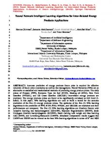
then PPL can regain both the universal approximation and convergence capabilities [107], based on results in [63]. This is also applicable to other algorithms using parametric hidden units. Experimentally, this modification also improves the rate of convergence with respect to the number of hidden units and gives better generalization performance [107]. For RPN, the convergence property has not been established. In fact, because its functional form is so different from traditional neural networks, typical universal approximation results (say, [53]–[56]) do not apply here. Its universal approximation capability, so far only with respect to the uniform norm, is proved in [95]. C. Cascade-Correlation In contrast to algorithms mentioned previously, algorithms in this section [83], [108]–[116], mostly variants of the cascade-correlation architecture [83] proposed by Fahlman and Lebiere, construct networks that have multiple hidden layers. This structural arrangement allows the development of powerful high-order feature detectors even with simple hidden units. Connectivity Scheme of the New Hidden Unit: The basic network architecture is typified by the cascade-correlation architecture. When a new hidden unit is to be created, besides establishing connection with each of the network’s original inputs and outputs, it also establishes connection with every existing hidden unit in the current network. Each new unit therefore adds a new one-unit “layer” to the network, leading to a cascade architecture (Fig. 4). Though typically used with simple hidden units, this cascade structure may also be combined with hidden units of more complicated transfer function. For example, in [109], each hidden unit is a local linear map that learns a linear approximation of the target function within its “receptive field.” Although the resultant deep network structure leads to the creation of very powerful high-order feature detectors, the number of connections for the th hidden unit increases as and gives rise to two major problems. 1) The generalization performance of the network may be degraded when is large, as it is likely that some of these parameters may be irrelevant to the prediction of the output. 2) There will be long propagation delays and an everincreasing fan-in of the hidden units as more units are added, making very large scale integration (VLSI) implementation difficult.


Fig. 4. The cascade-correlation architecture. In the diagram, empty circles represent input/hidden/output units while black dots refer to connections between units.

There are several possible methods to alleviate the first problem, which parallels the problem of controlling hidden unit complexity discussed in Section IV–B. For example, regularization may be used to reduce the effects of any spurious connections. Early success is reported in [117]. However, the regularization parameter must be manually set. A Bayesian method to set this automatically has been proposed in [104], leading to much-improved generalization performance. Another method is to prune the spurious connections. In [114], as each hidden unit is trained, the saliency of its weights is calculated and the weights that are determined to be weak are eliminated. This also partly alleviates the second problem. However, such an approach is computationally expensive and the saliency can only be approximated, sometimes with high error. A natural alternative is to limit the fan-in of the hidden units and connect the new hidden unit to only a selected few preexisting units. For example, in [111], Phatak and Koren modified the original cascade-correlation architecture by allowing more than one hidden unit in each layer, and each new hidden unit is connected only to the previous hidden layer. The fan-in of the hidden units is thus controlled by the number of units allowed in each hidden layer. When this maximum is reached and a new hidden unit is to be added, the current output layer is first collapsed into a new hidden layer, with further new hidden units added to this new layer. As a result, a regular multiple hidden layer structure is formed (Fig. 5). However, the maximum number of hidden units allowed in each layer may be crucial for performance. Restricting this to a small number limits the ability of the hidden units to form complicated feature detectors, as each hidden unit can only see its previous hidden layer outputs. With this restriction in mind, its universal approximation capability, even when the

639

Fig. 5. Modified cascade-correlation architecture with only partial connections.

number of hidden layers is allowed to grow without bound, seems unclear.8 An even more radical approach is to remove all cascade connections, reducing the resultant network to have only one single hidden layer [113], [116]. However, as only simple hidden units are employed in [113] and [116], they may have difficulty in learning complex problems (as mentioned in Section III-B). Training: Training for this class of algorithms is similar to that in Section IV-B. Only the new hidden unit is trained and training proceeds in a layer-by-layer manner. First, the weights feeding into the new hidden unit are trained (input training) by optimizing an objective function, while all the other weights in the network are kept fixed. Usually, there is a pool of such candidate hidden units, each using a different initial random seed. The candidate that optimizes the objective function in input training is installed into the network. After that, its weights are kept constant and only the weights connecting the hidden units to the output are trained (output training). When the output unit is linear, output training becomes a linear problem and the output layer weights may be conveniently obtained by computing the pseudoinverse exactly. A number of objective functions have been used in input training. For example, in the cascade-correlation architecture [83], the new hidden unit maximizes the covariance between the residual error and the hidden unit activation

where ranges over the training patterns, ranges over the output units, is the activation of the new hidden 8 In the extreme case when only one hidden unit is allowed in each layer, then obviously the universal approximation property does not hold.

640


unit for pattern , is the residual error at output for pattern before the new hidden unit is added, and and are the corresponding values averaged over all patterns. Some other correlation-based functions, with different time and space requirements, are proposed in [65] and [118]–[120]. The method mentioned in Section IV-B may also be used. An experimental comparison of the performance of these alternatives can be found in [120]. An exception is [110]. Here, the new hidden unit is treated as an interim output unit, as in the group method of data handling (GMDH) to be discussed in Section IV-E, and the error criterion is directly used to train the weights. Convergence Property: Except for the variant in [111], the universal approximation capability for this class of architectures is obvious, as these networks can be reduced to the regular single hidden layer networks by removing all cascade connections. The convergence property of the cascade-correlation algorithm, for networks using the hyperbolic tangent as hidden unit transfer function and the uniform input environment measure, is proved in [121]. More general results, extending to other hidden unit transfer functions, correlation functions in [118] and [120] and input environment measures, are discussed in [120]. However, for the criterion function in [65], the convergence property is not known. D. Resource-Allocating Network Similar to the algorithms in Sections IV-A and IV-B, algorithms in this class [122]–[125] also add hidden units to the same layer one at a time. However, the major difference is that memorization of training patterns is used to reduce the computational requirement of the training process, which is especially significant for constructive algorithms, as mentioned in Section III. Memorization has been used in methods like nearest neighbors and the Parzen windows [126]. However, these methods tend to produce networks that potentially grow linearly in the training set size, thus demanding large space and long time in computing network output. Algorithms in this section, typified by the resource-allocating network9 (RAN) developed by Platt [125], attempt to strike a good balance for the use of memorization. The central idea is to train the whole network only for the “easy” training patterns, while using memorization for the “hard” or “novel” patterns. Note that because memorization is based on individual patterns, training in these algorithms always proceeds in a pattern-by-pattern manner, compared to the other algorithms in which training may also proceed in a per-epoch manner. In RAN, a pattern is considered novel10 when it meets the following conditions. 1) It is farther away from all hidden units by a resolution parameter . 2) The difference between the desired output of the pattern and the network output is larger than the desired accuracy. Thus, if the network performs well on a particular training pattern, or if that pattern is already close to a stored vector, then 9A

function space approach to analyze RAN is developed in [127]. novelty detection methods may also be defined [128].

10 Other

the network adjusts its parameters. Otherwise, if the pattern is novel, it memorizes the input vector and the corresponding output vector of this pattern by allocating a new hidden unit. No training is required in this addition step. Note that these algorithms typically use RBF units as hidden units. An RBF unit responds to a small localized region of the input space. The explicit storage of an input–output pair as a new RBF unit means that this pair can be used immediately to improve system performance in a local region of the input space near this newly stored pair. On the other hand, a hidden unit with nonlocal response (such as a sigmoid unit) needs to undergo parameter update even for novel patterns, because it has a nonzero output for a large fraction of the training data. Another advantage of RAN and its variant [122] is that they can be used for sequential learning, i.e., training can commence before all training patterns have arrived. However, one problem with RAN is that noisy data may lead to a large number of hidden units. Moreover, the user-defined resolution parameter specifies the smallest distance two RBF units can have and features smaller than that will get averaged out. This effectively makes it impossible to appropriately model functions that vary on a finer scale. These problems are alleviated in the supervised growing cell structures [123]. Here, error information is accumulated in counters associated with each hidden unit. A new unit is inserted in regions with high local error only after presentation of a number of training patterns. Moreover, there is no hard threshold to control the minimum spacing between the RBF units. A major drawback of these algorithms is that their convergence properties are unknown. E. Group Method of Data Handling Constructive algorithms in this category [35], [49] are inspired by GMDH developed by Ivakhnenko [129]. The major difference from algorithms described in previous sections is that the state transition mapping is multivalued. Each hidden unit takes a fixed number of incoming connections, but the sources of these incoming connections are not fixed and may come from any possible combination of input and existing hidden units in the network. Thus, when a new hidden unit is to be added, there will be a number of candidate networks. Searching among these candidates can be done in different ways. For example, in [49], the search is done nondeterministically using simulated annealing. A state , corresponding to a network with the new hidden unit connected in a particular way, is randomly selected from among these candidates. An evaluation function , based on the MDL [45], is computed for . Denote the current state by . If , then is accepted; otherwise, will be accepted with , where is a “temperature” probability controlled by an annealing schedule. Alternatively, a simple greedy approach that chooses the candidate with the smallest eval value may be taken. The use of annealing, in contrast to the greedy approach, allows partial structures that look less than ideal to be accepted. But, on the other hand, annealing is less computationally efficient and becomes very timeconsuming in large problems. Another more ad hoc approach


641

F. Miscellaneous There are not many constructive algorithms that have multivalued state transition mappings while still retraining the whole network upon hidden unit addition, probably because of the consequent high computational requirement. Reference [130] is such an example. It is actually a hybrid algorithm with both constructive and pruning components. At each state, there are two new possible states,11 either by adding a new hidden unit to the same layer or by adding a whole hidden layer between the last hidden layer and the output layer. The number of hidden units in the new layer is heuristically set to be , where is the number of output units and is the number of hidden units in the last hidden layer. Selection between these two states is done by comparing the rate of change of the training error. Because of the ad hoc nature, the convergence property is not known. V. DISCUSSION Fig. 6. GMDH-type architecture.

is taken in [35]. Hidden units with training performance better than a user-determined threshold are all installed to the network. The resultant architecture is typically not a regular multiple hidden layer structure, but has many intralayer connections (Fig. 6). Training: As for algorithms in Sections IV-B and IV-C, only the new hidden unit is trained. But a characteristic of this class of algorithms is that the new hidden unit is treated as an interim output unit during training. As a result, there is only one layer of weights (i.e., those weights feeding into the hidden unit) to train. In principle, hidden units of any functional form may be used. However, training of each candidate hidden unit may be a nonlinear optimization problem. In this class of algorithms, further reduction in the computational requirement is achieved by the use of polynomial hidden units. Assume that there are incoming connections to the hidden unit, the transfer functions may be of the form

where and are the connection weights, and are the corresponding incoming activations. The number is usually set small, such as two. By treating the new hidden unit as an interim output unit and using the squared error as the error criterion, training of these connection weights reduces to a linear problem, and the weight solution may be obtained by simply computing the pseudoinverse. Approximation and Convergence Properties: Following from the well-known approximation properties for polynomials, GMDH networks are universal approximators even when the degree and the number of inputs to each hidden unit are constrained to be as small as two. However, because of the generally ad hoc nature of these types of algorithms, the convergence property is unknown.

AND

CONCLUSION

In this paper, we have reviewed the different algorithms used for constructing feedforward neural networks. Although the list of articles surveyed here is not exhaustive, one can still notice a conglomeration of various network architectures and training algorithms. The following issues may deserve particular attention. As discussed in Section III-B, the use of a greedy approach necessitates the ability of the algorithm to construct powerful feature detectors without using excessive parameters. This is achieved in various algorithms by using complicated hidden units (with the complexity coming from the use of either cascade connections or complicated functional forms). Regularization or subsequent pruning is then used to reduce the effective number of parameters. Other approaches may also be worth exploring. For example, one possibility is to start with simple hidden units, and when there is no significant reduction in residual error in a single state transition, the algorithm then increases the complexity of the hidden unit or trains several hidden units together in one single step. Moreover, as can be seen in the discussion in Section IV, convergence results are still lacking for a number of constructive algorithms, which definitely deserve more attention in the future. Going one step further, the rate of convergence is also an important theoretical yet crucial practical issue. Recent results [62], [63], [131]–[133] have shown that, under certain regularity conditions, the approximation error typically improves as , where is the number of hidden units in the network. However, as mentioned in Section II-D, some of these results are not applicable to constructive algorithms when a greedy approach is taken, whereas others are applicable to greedy algorithms but with the detailed conditions different from those used in practice. For example, in both [62] and [63], the iterative sequence of network estimates is formed from a convex combination of the previous network function and the new hidden unit function (7) 11 Actually,

there are four states, two of which are produced by the pruning component. However, in the following, we will focus our discussion on the constructive component and hence the pruning component will be ignored.

642

where . In algorithms like the cascade-correlation is formed algorithm (Section IV-C), however, the new from full linear combination of the old and new hidden unit functions. The weights connecting the old hidden units to the output unit are thus not constrained as a group, as in (7). must be learned together with the new Besides, in (7), hidden unit , while in the cascade-correlation algorithm, the parameters of the new hidden unit are first learned and then the output layer weights. Moreover, the objective function to be minimized in [62] and [63] is different from that in the cascade-correlation algorithm. Modifying and applying these useful theoretical results to the analysis of different constructive algorithms is thus beneficial. Some initial progress has been reported in [119]–[121]. As mentioned in Section II-C, one must decide when to stop the constructive algorithm. This is important to achieve a proper bias-variance tradeoff. A good stopping criterion will be one based on an estimate of the generalization performance of the network. But computing an accurate estimation efficiently for neural networks is not an easy problem to solve, and this will still be an important research topic. Up to now, a comprehensive performance comparison of different constructive algorithms is still lacking. Most of the reported works only compared a particular constructive algorithm with a fixed size network trained with traditional backpropagation. As different algorithms are suitable for different types of target functions, the identification of what class of target functions is most suitable for a particular constructive algorithm will be particularly useful from a practical point of view. Working along the same line of thought, the combination of several different constructive algorithms into a unified algorithm may be useful. This corresponds to a multivalued state transition mapping in the terminology of Section II-D. As can be seen in Sections IV-E and IV-F, there have only been a few attempts in this direction. Exploiting this kind of flexibility in a computationally efficient manner will thus be an interesting research direction. Also, the close link between constructive algorithms and forward stepwise regression techniques in statistics is worth mentioning. As discussed before, a number of constructive algorithms have been inspired by statistical techniques like PPR and GMDH. The problems of model selection and estimating generalization performance of neural networks also occur in a much wider context within statistics, and have been practised by statisticians for decades. The close relationship between various statistical methodologies and neural-network models has been discussed widely [23], [134]–[139], and there is still ongoing research to see how to borrow strength from each other. Finally, note that the various approaches to the control of network complexity, namely, regularization, and constructive and pruning algorithms, should not be treated as independent rivals. There are algorithms combining constructive and pruning algorithms [36], [85], [86], [91], [130], combining pruning and regularization [8], [140], combining regularization and constructive algorithms [104], and even combining all three [117]. Some of these have been mentioned in previous


sections. Thus, these approaches are complementary to each other and can work in a cooperative manner. ACKNOWLEDGMENT The authors would like to thank the anonymous reviewers for their constructive comments on an earlier version of this paper. REFERENCES [1] Y. Chauvin, “A backpropagation algorithm with optimal use of hidden units,” in Advances in Neural Information Processing Systems 1, D. S. Touretzky, Ed. San Mateo, CA: Morgan Kaufmann, 1989, pp. 519–526. [2] S. J. Hanson and L. Y. Pratt, “Comparing biases for minimal network construction with backpropagation,” in Advances in Neural Information Processing Systems 1, D. S. Touretzky, Ed. San Mateo, CA: Morgan Kaufmann, 1989, pp. 177–185. [3] A. S. Weigend, D. E. Rumelhart, and B. A. Huberman, “Generalization by weight-elimination with application to forecasting,” in Advances in Neural Information Processing Systems 3, R. Lippmann, J. Moody, and D. Touretzky, Eds. San Mateo, CA: Morgan Kaufmann, 1991, pp. 875–882. [4] G. H. Golub, M. Heath, and G. Wahba, “Generalized cross-validation as a method for choosing a good ridge parameter,” Technometrics, vol. 21, no. 2, pp. 215–223, 1979. [5] W. L. Buntine and A. S. Weigend, “Bayesian backpropagation,” Complex Syst., vol. 5, pp. 603–643, 1991. [6] D. J. C. Mackay, “Bayesian interpolation,” Neural Computa., vol. 4, no. 3, pp. 415–447, May 1992. [7] R. M. Neal, “Bayesian learning for neural networks,” Ph.D. dissertation, Dep. Computer Sci., Univ. Toronto, Canada, 1995. [8] H. H. Thodberg, “A review of Bayesian neural networks with an application to near infrared spectroscopy,” IEEE Trans. Neural Networks, vol. 7, pp. 56–72, 1996. [9] P. M. Williams, “Bayesian regularization and pruning using a Laplace prior,” Neural Computa., vol. 7, pp. 117–143, 1995. [10] D. J. C. MacKay, “A practical Bayesian framework for backpropagation networks,” Neural Computa., vol. 4, no. 3, pp. 448–472, May 1992. [11] J. S. Judd, Neural Network Design and the Complexity of Learning. Cambridge, MA: MIT Press, 1990. [12] A. L. Blum and R. L. Rivest, “Training a 3-node neural network is NP-complete,” Neural Networks, vol. 5, pp. 117–127, 1992. [13] J. H. Lin and J. S. Vitter, “Complexity results on learning by neural nets,” Machine Learning, vol. 6, pp. 211–230, 1991. [14] J. Sima, “Loading deep networks is hard,” Neural Computa., vol. 6, pp. 842–850, 1994. [15] E. B. Baum, “Book review on ‘Neural-network design and the complexity of learning,’” IEEE Trans. Neural Networks, vol. 2, pp. 181–182, 1991. [16] L. G. Valiant, “A theory of the learnable,” Commun. ACM, vol. 27, no. 11, pp. 1134–1142, 1984. [17] E. B. Baum, “A proposal for more powerful learning algorithms,” Neural Computa., vol. 1, no. 2, pp. 201–207, 1989. [18] R. Reed, “Pruning algorithms—A survey,” IEEE Trans. Neural Networks, vol. 4, pp. 740–747, Sept. 1993. [19] E. D. Karnin, “A simple procedure for pruning backpropagation trained neural networks,” IEEE Trans. Neural Networks, vol. 1, pp. 239–242, June 1990. [20] M. C. Mozer and P. Smolensky, “Skeletonization: A technique for trimming the fat from a network via relevance assessment,” in Advances in Neural Information Processing Systems 1, D. S. Touretzky, Ed. San Mateo, CA: Morgan Kaufmann, 1989, pp. 107–115. [21] B. Hassibi and D. G. Stork, “Second-order derivatives for network pruning: Optimal brain surgeon,” in Advances in Neural Information Processing Systems 5. San Mateo, CA: Morgan Kaufmann, 1993, pp. 164–171. [22] Y. Le Cun, J. S. Denker, and S. A. Solla, “Optimal brain damage,” in Advances in Neural Information Processing Systems 2, D. S. Touretzky, Ed. San Mateo, CA: Morgan Kaufmann, 1990, pp. 598–605. [23] J. H. Friedman, “An overview of predictive learning and function approximation,” in From Statistics to Neural Networks: Theory and Pattern Recognition Applications, J. H. Friedman and H. Wechsler, Eds., ASI Proc., Subseries F. New York: Springer-Verlag, 1994.


[24] E. Alpaydin, “GAL: Networks that grow when they learn and shrink when they forget,” Int. Computer Sci. Inst., Berkeley, CA, Tech. Rep. 91-032, May 1991. [25] G. Deffuant, “Neural units recruitment algorithm for generation of decision trees,” in Proc. 1990 IEEE Int. Joint Conf. Neural Networks, San Diego, CA, vol. 1, June 1990, pp. 637–642. [26] M. Frean, “The upstart algorithm: A method for constructing and training feedforward neural networks,” Neural Computa., vol. 2, pp. 198–209, 1990. [27] M. Marchand, M. Golea, and P. Ruj´an, “A convergence theorem for sequential learning in two-layer perceptrons,” Europhys. Lett., vol. 11, no. 6, pp. 487–492, 1990. [28] T. Ash and G. Cottrell, “Topology modifying neural network algorithms,” in Handbook of Brain Theory and Neural Networks, M. A. Arbib, Ed. Cambridge, MA: MIT Press, 1995, pp. 990–993. [29] T. Ash and G. W. Cottrell, “A review of learning algorithms that modify network topologies,” Computer Sci. Eng., Univ. California, San Diego, Tech. Rep. CS94-348, 1994. [30] E. Fiesler, “Comparative bibliography of ontogenic neural networks,” in Proc. Int. Conf. Artificial Neural Networks, Sorrento, Italy, vol. 1, May 1994, pp. 793–796. [31] D. E. Nelson and S. K. Rogers, “A taxonomy of neural network optimality,” in Proc. IEEE Nat. Aerospace Electron. Conf., Dayton, OH, vol. 3, May 1992, pp. 894–899. [32] G. Gong, “Cross-validation, the jackknife, and the bootstrap: Excess error estimation in forward logistic regression,” J. Amer. Statist. Assoc., vol. 81, no. 393, pp. 108–113, May 1986. [33] A. R. Barron, “Approximation and estimation bounds for artificial neural networks,” Machine Learning, vol. 14, pp. 115–133, 1994. [34] S. Geman, E. Bienenstock, and R. Doursat, “Neural networks and the bias/variance dilemma,” Neural Computa., vol. 4, pp. 1–58, 1992. [35] R. E. Parker and M. Tummala, “Identification of Volterra systems with a polynomial neural network,” in Proc. 1992 IEEE Int. Conf. Acoust., Speech, Signal Processing, San Francisco, CA, vol. 4, Mar. 1992, pp. 561–564. [36] J. Moody, “Prediction risk and architecture selection for neural networks,” in From Statistics to Neural Networks: Theory and Pattern Recognition Applications, V. Cherkassky, J. H. Friedman, and H. Wechsler, Eds., vol. 136 of NATO ASI Series F. New York: SpringerVerlag, 1994, pp. 147–165. [37] M. Stone, “Cross-validatory choice and assessment of statistical predictions (with discussion),” J. Roy. Statist. Soc. Series B, vol. 36, pp. 111–147, 1974. [38] B. Efron and R. J. Tibshirani, An Introduction to the Bootstrap, vol. 57 of Monographs on Statistics and Applied Probability. New York: Chapman and Hall, 1993. [39] A. S. Weigend and B. LeBaron, “Evaluating neural network predictors by bootstrapping,” in Proc. Int. Conf. Neural Inform. Processing, Seoul, Korea, vol. 2, Oct. 1994, pp. 1207–1212. [40] H. Akaike, “A new look at the statistical model identification,” IEEE Trans. Automat. Contr., vol. AC-19, pp. 716–723, Dec. 1974. [41] G. Schwartz, “Estimating the dimension of a model,” Ann. Statist., vol. 6, pp. 461–464, 1978. [42] H. Akaike, “Statistical predictor identification,” Ann. Instit. Statist. Math., vol. 22, pp. 203–217, 1970. [43] P. Craven and G. Wahba, “Smoothing noisy data with spline functions: Estimating the correct degree of smoothing by the method of generalized cross-validation,” Numer. Math., vol. 31, pp. 377–403, 1979. [44] A. Barron, “Predicted squared error: A criterion for automatic model selection,” in Self-Organizing Methods in Modeling, S. Farlow, Ed. New York: Marcel Dekker, 1984. [45] J. Rissanen, “Modeling by shortest data description,” Automatica, vol. 14, pp. 465–471, 1975. [46] J. E. Moody, “Note on generalization, regularization, and architecture selection in nonlinear learning systems,” in Proc. 1991 IEEE Wkshp. Neural Networks for Signal Processing, B. H. Juang, S. Y. Kung, and C. A. Kamm, Eds. Princeton, NJ,, Sept. 1991, pp. 1–10. [47] B. D. Ripley, “Choosing network complexity,” in Probabilistic Reasoning and Bayesian Belief Networks, A. Gammerman, Ed., 1995, pp. 97–108. [48] B. D. Ripley, “Statistical ideas for selecting network architectures,” in Neural Networks: Artificial Intelligence and Industrial Applications, B. Kappen and S. Gielen, Eds. New York: Springer-Verlag, 1995, pp. 183–190. [49] M. F. Tenorio and W. T. Lee, “Self-organizing network for optimum supervised learning,” IEEE Trans. Neural Networks, vol. 1, pp. 100–110, Mar. 1990.

643

[50] E. Hartman and J. D. Keeler, “Predicting the future: Advantages of semilocal units,” Neural Computa., vol. 3, pp. 566–578, 1991. [51] J. Moody and C. Darken, “Learning with localized receptive fields,” in Proc. 1988 Connectionist Models Summer School, 1988, pp. 133–143. [52] S. Renals, “Radial basis function network for speech pattern classification,” Electron. Lett., vol. 25, no. 7, pp. 437–439, 1988. [53] G. Cybenko, “Approximation by superpositions of a sigmoidal function,” Math. Contr., Signals, Syst., vol. 2, pp. 303–314, 1989. [54] K. I. Funahashi, “On the approximate realization of continous mappings by neural networks,” Neural Networks, vol. 2, pp. 183–192, 1989. [55] K. Hornik, “Approximation capabilities of multilayer feedforward networks,” Neural Networks, vol. 4, pp. 251–257, 1991. [56] , “Some new results on neuralnetwork approximation,” Neural Networks, vol. 6, pp. 1069–1072, 1993. [57] E. Hartman, J. Keeler, and J. Kowalski, “Layered neural networks with Gaussian hidden units as universal approximations,” Neural Computa., vol. 2, pp. 210–215, 1990. [58] J. Park and I. Sandberg, “Universal approximation using radial-basisfunction networks,” Neural Computa., vol. 3, pp. 246–257, 1991. [59] , “Approximation and radial-basis-function networks,” Neural Computa., vol. 5, pp. 305–316, 1993. [60] A. N. Kolmogorov and S. V. Fomin, Introductory Real Analysis. New York: Dover, 1975. [61] G. Lugosi and K. Zeger, “Nonparametric estimation via empirical risk minimization,” IEEE Trans. Inform. Theory, vol. 41, pp. 677–687, May 1995. [62] A. R. Barron, “Universal approximation bounds for superpositions of a sigmoidal function,” IEEE Trans. Inform. Theory, vol. 39, pp. 930–945, May 1993. [63] L. K. Jones, “A simple lemma on greedy approximation in Hilbert space and convergence rates for projection pursuit regression and neural network training,” Ann. Statist., vol. 20, no. 1, pp. 608–613, 1992. [64] F. L. Chung and T. Lee, “Network-grwoth approach to design of feedforward neural networks,” in IEE Proceedings. Control Theory and Applications, Sept. 1995. [65] P. Courrieu, “A convergent generator of neural networks,” Neural Networks, vol. 6, no. 6, pp. 835–844, 1993. [66] J. Luo, “A bias architecture with rank-expanding algorithm for neural networks supervised learning problem,” in Proc. World Congr. Neural Networks, San Diego, CA, vol. 3, June 1994, pp. 742–747. [67] G. Weiss, “Neural networks and evolutionary computation—Part 1: Hybrid approaches in artificial intelligence,” in Proc. 1st IEEE Conf. Evolutionary Computa., Orlando, FL, vol. 1, June 1994, pp. 268–272. [68] X. Yao, “A review of evolutionary artificial neural networks,” Int. J. Intell. Syst., vol. 8, pp. 539–567, 1993. [69] G. F. Miller, P. M. Todd, and S. U. Hegde, “Designing neural networks using genetic algorithms,” in Proc. 3rd Int. Conf. Genetic Algorithms, 1989, pp. 379–384. [70] C. C. Teng and B. W. Wah, “An automated design system for finding the minimal configuration of a feedforward neural network,” in Proc. IEEE Int. Conf. Neural Networks, Orlando, FL, vol. 3, June 1994, pp. 1295–1300. [71] R. Battiti, “First- and second-order methods for learning: Between steepest descent and Newton’s method,” Neural Computa., vol. 4, pp. 141–166, 1992. [72] T. T. Jervis and W. J. Fitzgerald, “Optimization schemes for neural networks,” Cambridge Univ. Eng. Dep., Cambridge, U.K., Rep. CUED/F-INFENG/TR 144, 1993. [73] W. H. Press, S. A. Teukolsky, W. T. Vetterling, and B. P. Flannery, Numerical Recipes in C, 2nd ed. New York: Cambridge Univ. Press, 1992. [74] L. Xu, S. Klasa, and A. Yuille, “Recent advances on techniques of static feedforward networks with supervised learning,” Int. J. Neural Syst., vol. 3, no. 3, pp. 253–290, 1992. [75] G. S. G. Beveridge and R. S. Schechter, Optimization: Theory and Practice New York: McGraw-Hill, 1970. [76] SAS Institute Inc., SAS/STAT User’s Guide, release 6.03 edition, 1988. [77] M. R. Azimi-Sadjadi, S. Sheedvash, and F. O. Trujillo, “Recursive dynamic node creation in multilayer neural networks,” IEEE Trans. Neural Networks, vol. 4, pp. 242–256, Mar. 1993. [78] P. S. Lewis and J. N. Hwang, “Recursive least-squares learning algorithms for neural networks,” in Proc. SPIE Advanced Signal-Processing Algorithms, Architectures, and Implementations, vol. 1348, 1990, pp. 28–39. [79] S. E. Fahlman, “Faster learning variations on backpropagation: An empirical study,” in Proc. 1988 Connectionist Models Summer School, D. S. Touretzky, G. E. Hinton, and T. J. Sejnowski, Eds. San Mateo, CA: Morgan Kaufmann, 1988, pp. 38–51.

644

[80] R. Setiono and L. C. K. Hui, “Use of a quasi-Newton method in a feedforward neural network construction algorithm,” IEEE Trans. Neural Networks, vol. 6, pp. 273–277, 1995. [81] J. H. Friedman and W. Stuetzle, “Projection pursuit regression,” J. Amer. Statist. Assoc., vol. 76, no. 376, pp. 817–823, 1981. [82] S. Sjøgaard, “A conceptual approach to generalization in dynamic neural networks,” Ph.D. dissertation, Computer Sci. Dep., Aarhus University, Aarhus, Denmark, 1991. [83] S. E. Fahlman and C. Lebiere, “The cascade-correlation learning architecture,” in Advances in Neural Information Processing Systems 2, D. S. Touretzky, Ed. San Mateo, CA: Morgan Kaufmann, pp. 524–532, 1990. [84] T. Ash, “Dynamic node creation in backpropagation networks,” Connection Sci., vol. 1, no. 4, pp. 365–375, 1989. [85] E. B. Bartlett, “Dynamic node architecture learning: An information theoretic approach,” Neural Networks, vol. 7, no. 1, pp. 129–140, 1994. [86] Y. Hirose, K. Yamashita, and S. Hijiya, “Backpropagation algorithm which varies the number of hidden units,” Neural Networks, vol. 4, pp. 61–66, 1991. [87] K. Khorasani and W. Weng, “Structure adaptation in feedforward neural networks,” in Proc. IEEE Int. Conf. Neural Networks, Orlando, FL, vol. 3, June 1994, pp. 1403–1408. [88] B. T. Zhang, “An incremental learning algorithm that optimizes network size and sample size in one trial,” in Proc. IEEE Int. Conf. Neural Networks, Orlando, FL, vol. 1, June 1994, pp. 215–220. [89] T. E. Flick, L. K. Jones, R. G. Priest, and C. Herman, “Pattern classification using projection pursuit,” Pattern Recognition, vol. 23, no. 12, pp. 1367–1376, 1990. [90] J. H. Friedman, E. Grosse, and W. Stuetzle, “Multidimensional additive spline approximation,” SIAM J. Sci. Statist. Computing, vol. 4, no. 2, pp. 291–301, June 1983. [91] J. N. Hwang, S. R. Lay, M. Maechler, D. Martin, and J. Schimert, “Regression modeling in backpropagation and projection pursuit learning,” IEEE Trans. Neural Networks, vol. 5, pp. 342–353, May 1994. [92] S. Lay, J. Hwang, and S. You, “Extensions to projection pursuit learning networks with parametric smoothers,” in Proc. IEEE Int. Conf. Neural Networks, Orlando, FL, vol. 3, June 1994, pp. 1325–1330. [93] C. B. Roosen and T. J. Hastie, “Automatic smoothing spline projection pursuit,” J. Computa. Graphical Statist., vol. 3, pp. 235–248, 1994. [94] A. Saha, C. L. Wu, and D. S. Tang, “Approximation, dimension reduction, and nonconvex optimization using linear superpositions of Gaussians,” IEEE Trans. Computers, vol. 42, pp. 1222–1233, Oct. 1993. [95] Y. Shin and J. Ghosh, “Ridge polynomial networks,” IEEE Trans. Neural Networks, vol. 6, May 1995. [96] W. Verkooijen and H. Daniels, “Connectionist projection pursuit regression,” Computa. Economics, vol. 7, pp. 155–161, 1994. [97] J. L. Yuan and T. L. Fine, “Forecasting demand for electric power,” in Advances in Neural Information Processing Systems 5, S. J. Hanson, J. D. Cowan, and C. L. Giles, Eds. San Mateo, CA: Morgan Kaufmann, 1993, pp. 739–746. [98] Y. Zhao and C. G. Atkeson, “Some approximation properties of projection pursuit learning networks,” in Advances in Neural Information Processing Systems 4, J. E. Moody, S. J. Hanson, and R. P. Lippman, Eds. San Mateo, CA: Morgan Kaufmann, 1992, pp. 936–943. [99] Statistical Sciences, Inc., Seattle, WA, S-Plus User’s Manual, 3rd ed., Sept. 1991. [100] J. Moody and N. Yarvin, “Networks with learned unit response functions,” in Advances in Neural Information Processing Systems 4, J. E. Moody, S. J. Hanson, and R. P. Lippmann, Eds. San Mateo, CA: Morgan Kaufmann, 1992, pp. 1048–1055. [101] J. H. Friedman, “Exploratory projection pursuit,” J. Amer. Statist. Assoc., vol. 82, no. 397, pp. 249–266, Mar. 1987. [102] Y. Shin and J. Ghosh, “The pi-sigma network: An efficient higher-order neural network for pattern classification and function approximation,” in Proc. Int. Joint Conf. Neural Networks, Seattle, WA, vol. 1, July 1991, pp. 13–18. [103] N. Intrator, “Combining exploratory projection pursuit and projection pursuit regression with application to neural networks,” Neural Computa., vol. 5, pp. 443–455, May 1993. [104] T. Y. Kwok and D. Y. Yeung, “Bayesian regularization in constructive neural networks,” in Proc. Int. Conf. Artificial Neural Networks, Bochum, Germany, July 1996, pp. 557–562. [105] J. Ghosh and Y. Shin, “Efficient higher-order neural networks for classification and function approximation,” Int. J. Neural Syst., vol. 3, no. 4, pp. 323–350, 1992. [106] L. K. Jones, “On a conjecture of Huber concerning the convergence of projection pursuit regression,” Ann. Statist., vol. 15, no. 2, pp. 880–882, 1987.


[107] T. Y. Kwok and D. Y. Yeung, “Use of bias term in projection pursuit learning improves approximation and convergence properties,” IEEE Trans. Neural Networks, vol. 7, pp. 1168–1183, 1996. [108] W. Fang and R. C. Lacher, “Network complexity and learning efficiency of constructive learning algorithms,” in Proc. IEEE Int. Conf. Neural Networks, Orlando, FL, vol. 1, June 1994, pp. 366–369. [109] E. Littmann and H. Ritter, “Cascade LLM networks,” in Proc. Int. Conf. Artificial Neural Networks, Brighton, U.K., vol. 1, Sept. 1992, pp. 253–257. [110] , “Cascade network architectures,” in Proc. Int. Joint Conf. Neural Networks, Baltimore, MD, vol. 2, June 1992, pp. 398–404. [111] D. S. Phatak and I. Koren, “Connectivity and performance tradeoffs in the cascade correlation learning architecture,” IEEE Trans. Neural Networks, vol. 5, pp. 930–935, Nov. 1994. [112] N. Simon, H. Corporaal, and E. Kerckhoffs, “Variations on the cascadecorrelation learning architecture for fast convergence in robot control,” in Proc. 5th Int. Conf. Neural Networks Applicat., Nimes, France, Nov. 1992, pp. 454–464. [113] S. Sjøgaard, “Generalization in cascade-correlation networks,” in Proc. IEEE—SP Wkshp. Neural Networks for Signal Processing II, Helsingoer, Denmark, Sept. 1992, pp. 59–68. [114] I. G. Smotroff, D. H. Friedman, and D. Connolly, “Self organizing modular neural networks,” in Proc. Int. Joint Conf. Neural Networks, Seattle, WA, July 1991. [115] P. L. Springer and S. Gulati, “Parallelizing the cascade-correlation algorithm using time warp,” Neural Networks, vol. 8, no. 4, pp. 571–577, 1995. [116] D. Y. Yeung, “A neural network approach to constructive induction,” in Proc. 8th Int. Wkshp. Machine Learning, Evanston, IL, 1991. [117] L. K. Hansen and M. W. Pedersen, “Controlled growth of cascade correlation nets,” in Proc. Int. Conf. Artificial Neural Networks, Sorrento, Italy, vol. 1, May 1994, pp. 797–800. [118] O. Fujita, “Optimization of the hidden unit function in feedforward neural networks,” Neural Networks, vol. 5, pp. 755–764, 1992. [119] V. Kurkov´a and B. Beliczynski, “Incremental approximation by onehidden-layer neural networks,” in Proc. Int. Conf. Artificial Neural Networks, Paris, France, vol. 1, Oct. 1995, pp. 5505–5510. [120] T. Y. Kwok and D. Y. Yeung, “Objective functions for training new hidden units in constructive neural networks,” submitted to IEEE Trans. Neural Networks. [121] G. P. Drago and S. Ridella, “Convergence properties of cascade correlation in function approximation,” Neural Comput. Applicat., vol. 2, pp. 142–147, 1994. [122] G. Deco and J. Ebmeyer, “Coarse coding resource-allocating network,” Neural Computa., vol. 5, pp. 105–114, 1993. [123] B. Fritzke, “Growing cell structures—A self-organizing network for unsupervised and supervised learning,” Neural Networks, vol. 7, no. 9, pp. 1441–1460, 1994. [124] S. Lee and R. M. Kil, “A Gaussian potential function network with hierarchically self-organizing learning,” Neural Networks, vol. 4, pp. 207–224, 1991. [125] J. Platt, “A resource-allocating network for function interpolation,” Neural Computa., vol. 3, pp. 213–225, 1991. [126] R. O. Duda and P. E. Hart, Pattern Classification and Scene Analysis. New York: Wiley, 1973. [127] V. Kadirkamanathan and M. Niranjan, “A function estimation approach to sequential learning with neural networks,” Neural Computa., vol. 5, no. 6, pp. 954–975, 1993. [128] S. Roberts and L. Tarassenko, “A probabilistic resource allocating network for novelty detection,” Neural Computa., vol. 6, no. 2, pp. 270–284, Mar. 1994. [129] S. J. Farlow, Ed., Self-Organizing Methods in Modeling: GMDH Type Algorithms, vol. 54 of Statistics: Textbooks and Monographs. New York: Marcel Dekker, 1984. [130] T. M. Nabhan and A. Y. Zomaya, “Toward generating neural network structures for function approximation,” Neural Networks, vol. 7, no. 1, pp. 89–90, 1994. [131] C. Darken, M. Donahue, L. Gurvits, and E. Sontag, “Rate of approximation results motivated by robust neural network learning,” Siemens Corporate Res., Inc., Princeton, NJ, Tech. Rep., Apr. 1994. [132] K. Hornik, M. Stinchcombe, H. White, and P. Auer, “Degree of approximation results for feedforward networks approximating unknown mappings and their derivations,” Neural Computa., vol. 6, pp. 1262–1275, 1994. [133] L. Xu, A. Krzyzak, and A. Yuille, “On radial basis function nets and kernel regression: Statistical consistency, convergence rates, and receptive field size,” Neural Networks, vol. 7, no. 4, pp. 609–628, 1994.


[134] A. R. Barron and R. L. Barron, “Statistical learning networks: A unifying view,” in Proc. 20th Symp. Interface Computing Sci. Statist., E. Wegman, Ed. Washington, D.C.: Amer. Statist. Assoc., 1988, pp. 192–203. [135] B. Cheng and D. M. Titterington, “Neural networks: A review from a statistical perspective (with discussion),” Statist. Sci., vol. 9, no. 1, pp. 2–54, 1994. [136] V. Cherkassky, “Neural networks and nonparametric regression,” in Proc. IEEE-SP Wkshp., Helsingoer, Denmark, Aug. 1992, pp. 511–521. [137] B. D. Ripley, “Statistical aspects of neural networks,” in Networks and Chaos—Statistical and Probabilistic Aspects, O. E. Barndorff-Nielsen, J. L. Jensen, and W. S. Kendall, Eds. London: Chapman and Hall, 1993, pp. 40–123. [138] B. D. Ripley, “Neural networks and related methods for classification (with discussion),” J. Roy. Statist. Soc. Series B, vol. 56, 1994. [139] W. S. Sarle, “Neural networks and statistical models,” in Proc. 19th Annu. SAS Users Group Int. Conf., Apr. 1994. [140] D. J. C. MacKay, “Probable networks and plausible predictions—A review of practical Bayesian methods for supervised neural networks,” Network: Computa. Neural Syst., vol. 6, no. 3, pp. 469–505, Aug. 1995.

Tin-Yau Kwok received the B.Sc. (Eng.) degree from the University of Hong Kong and the Ph.D. degree in computer science from the Hong Kong University of Science and Technology. He is with the Department of Computer Science, Hong Kong University of Science and Technology. His current research interests include artificial neural networks, pattern recognition, and Bayesian statistics.

645

Dit-Yan Yeung (S’82–M’90) received the B.Sc. (Eng.) degree in electrical engineering and M.Phil. degree in computer science from the University of Hong Kong, and the Ph.D. degree in computer science from the University of Southern California, Los Angeles. He is currently an Assistant Professor in the Hong Kong University of Science and Technology. His current research interests include neural computation, statistical learning theory, and handwriting recognition.

Constructive Algorithms For Structure Learning In Feedforward Neural ...

Constructive Algorithms For Structure Learning In Feedforward Neural ...

Suggest Documents

Constructive Feedforward Neural Networks for ... - CiteSeerX

A Constructive Algorithm for Feedforward Neural ...

Constructive Feedforward Neural Networks for ... - CiteSeerX

Dynamic Constructive Fault Tolerant Algorithm for Feedforward Neural

Training Feedforward Neural Networks Using Genetic Algorithms

analysis of feedforward and recurrent neural network algorithms in ...

A Constructive Spiking Neural Network for Reinforcement Learning in ...

Brain-Inspired Constructive Learning Algorithms with

Global Feedforward Neural Network Learning For Classification And ...

Neural Network Intelligent Learning Algorithms for ...

Neural Network Intelligent Learning Algorithms for ...

Supervised Learning in Feedforward Artificial Neural ... - Google Sites

Topology design of feedforward neural networks by genetic algorithms

Universal Approximation Using Incremental Constructive Feedforward ...

Universal Approximation Using Incremental Constructive Feedforward ...

a comparison of constructive and pruning algorithms to design neural

Constructive Neural Network Algorithms that Solve Highly ... - CiteSeerX

Constructive Neural Networks - CiteSeerX

Optimal Unsupervised Learning in Feedforward

Feedforward neural networks for nonparametric regression

Evolving Neural Feedforward Networks - CiteSeerX

Evolving Neural Feedforward Networks - CiteSeerX

Simplified Stochastic Feedforward Neural Networks

Constructive Algorithms for Hierarchical Mixtures ... - Semantic Scholar