Oct 3, 2016 - He showed that this kind of generalized s.i.p. space induces a norm by setting x ... In our paper we call Lorentzian space the Minkowski space defined by an ..... Its centre will be the pole of the dividing circle, and its principal.
CONSTRUCTIVE CURVES IN NON-EUCLIDEAN GEOMETRIES ´ ´ AKOS G.HORVATH
arXiv:1610.00473v1 [math.MG] 3 Oct 2016
Abstract. In this paper we overview the theories of conics and roulettes in four non-Euclidean planes, respectively. We collected the literature connected with these classical concepts from the eighteenth century to the present mentioned papers available only on the ArXiv, too.
Keywords: angle measure; Cayley-Klein geometries; conics; Euler-Savary equations; normed plane; roulettes 2010 MSC: 46B20, 51M05, 52A21, 53A17 1. Introduction In this survey we review two types of constructive curves in certain non-Euclidean planes. We organize our paper as follows: firstly we are placing the chosen geometries in the map of ”plane geometries” than we compare the theories of the examined constructive curves to each other. It is clear that we cannot mention all results discovered in the last three hundred years, however there are some important characteristic with analogous forms in these geometries, we concentrate on these. Very important to know what kind of definitions work simultaneously, how can we classify the conics and how work the basic kinematics in these non-Euclidean planes, respectively. We also give a large number of references can be found in that place of the paper when it have to cite. 2. On the map of the plane geometries We require an analytic approach to the investigated geometries so we cannot mention here such nonEuclidean planes which has only synthetic building up (for example non-Paschian planes based on a synthetic construction as we can find in [35]). The common roof of the four geometries the so-called hyperbolic, spherical, Minkowski and Lorentzian, geometries is a 3-dimensional vector space endowed with a general scalar multiplication of the vectors. This multiplication is a function with two arguments on V × V to the reals is calling by product. First we review a possibility to axiomatize it. 2.1. The two Minkowski planes as affine spaces and their common building up. A generalization of the inner product and the inner product spaces (briefly i.p spaces) was raised by G. Lumer in [47]. Definition 1 ([47]). The semi-inner-product (s.i.p) on a complex vector space V is a complex function [x, y] : V × V −→ C with the following properties: s1: s2: s3: s4:
: : : :
[x + y, z] = [x, z] + [y, z], [λx, y] = λ[x, y] for every λ ∈ C, [x, x] > 0 when x 6= 0, |[x, y]|2 ≤ [x, x][y, y],
A vector space V with a s.i.p. is an s.i.p. space. p G. Lumer proved that an s.i.p space is a normed vector space with norm kxk = [x, x] and, on the other hand, that every normed vector space can be represented as an s.i.p. space. In [25] J. R. Giles showed that the following homogeneity property holds: ¯ y] for all complex λ. s5: : [x, λy] = λ[x, This can be imposed, and all normed vector spaces can be represented as s.i.p. spaces with this property. Giles also introduced the concept of continuous s.i.p. space as an s.i.p. space having the additional property Date: Sept, 2016. 1
´ G.HORVATH ´ A.
2
s6: : For any unit vectors x, y ∈ S, Re{[y, x + λy]} → Re{[y, x]} for all real λ → 0. The space is uniformly continuous if the above limit is reached uniformly for all points x, y of the unit sphere S. A characterization of the continuous s.i.p. space is based on the differentiability property of the space. Definition 2 ([25]). A normed space is Gˆ ateaux differentiable if for all elements x, y of its unit sphere and real values λ, the limit kx + λyk − kxk lim λ→0 λ exists. A normed vector space is uniformly Fr`echet differentiable if this limit is reached uniformly for the pair x, y of points from the unit sphere. Giles proved in [25] that Theorem 1 ([25]). An s.i.p. space is a continuous (uniformly continuous) s.i.p. space if and only if the norm is Gˆ ateaux (uniformly Fr`echet) differentiable. B. Nath gave in [56] a straightforward generalization of an s.i.p., by replacing the Cauchy-Schwartz inequality by H¨ older’s inequality. He showed that this kind of generalized s.i.p. space induces a norm 1 by setting kxk = [x, x] p 1 ≤ p ≤ ∞, and that for every normed space a generalized s.i.p. space can be constructed. (For p = 2, this theorem reduces to Theorem 2 of Lumer.) The connection between the Lumer-Giles s.i.p. and the generalized s.i.p. of Nath is simple. For any p, the s.i.p. [x, y] defines a generalized s.i.p. by the equality p−2 [ [x, y] = [y, y] p [x, y]. The s.i.p. has the homogeneity property of Giles if and only if Nath’s generalized s.i.p. satisfies the (p − 1)-homogeneity property \ [ ¯ p−2 [x, s5”: : [x, λy] = λ|λ| y] for all complex λ.
Thus, in this paper we will concentrate only to the original version of the s.i.p.. From the geometric point of view we know that if K is a 0-symmetric, bounded, convex body in the Euclidean n-space Rn (with fixed origin O), then it defines a norm whose unit ball is K itself (see [39]). Such a space is called Minkowski space or normed linear space. Basic results on such spaces are collected in the surveys [50], [51], and [49]. In fact, the norm is a continuous function which is considered (in geometric terminology, as in [39]) as a gauge function. Combining this with the result of Lumer and Giles we get that a normed linear space can be represented as an s.i.p space. The metric of such a space (called Minkowski metric), i.e. the distance of two points induced by this norm, is invariant with respect to translations. Another concept of Minkowski space was also raised by H. Minkowski and used in Theoretical Physics and Differential Geometry, based on the concept of indefinite inner product. (See, e.g., [24].) Definition 3 ([24]). The indefinite inner product (i.i.p.) on a complex vector space V is a complex function [x, y] : V × V −→ C with the following properties: i1: i2: i3: i4:
: : : :
[x + y, z] = [x, z] + [y, z], [λx, y] = λ[x, y] for every λ ∈ C, [x, y] = [y, x] for every x, y ∈ V , [x, y] = 0 for every y ∈ V then x = 0.
A vector space V with an i.i.p. is called an i.i.p. space. We recall, that a subspace of an i.i.p. space is positive (non-negative) if all of its nonzero vectors have positive (non-negative) scalar squares. The classification of subspaces of an i.i.p. space with respect to the positivity property is also an interesting question. First we pass to the class of subspaces which are peculiar to i.i.p. spaces, and which have no analogous in the spaces with a definite inner product. Definition 4 ([24]). A subspace N of V is called neutral if [v, v] = 0 for all v ∈ N . In view of the identity 1 [x, y] = {[x + y, x + y] + i[x + iy, x + iy] − [x − y, x − y] − i[x − iy, x − iy]}, 4
CONSTRUCTIVE CURVES IN NON-EUCLIDEAN GEOMETRIES
3
a subspace N of an i.i.p. space is neutral if and only if [u, v] = 0 for all u, v ∈ N . Observe also that a neutral subspace is non-positive and non-negative at the same time, and that it is necessarily degenerate. Therefore the following statement can be proved. Theorem 2 ([24]). An non-negative (resp. non-positive) subspace is the direct sum of a positive (resp. negative) subspace and a neutral subspace. We note that the decomposition of a non-negative subspace U into a direct sum of a positive and a neutral component is, in general, not unique. However, the dimension of the positive summand is uniquely determined. The standard mathematical model of space-time is a four dimensional i.i.p. space with signature (+, +, +, −), also called Minkowski space in the literature. Thus we have a well known homonyms with the notion of Minkowski space! In our paper we call Lorentzian space the Minkowski space defined by an indefinite scalar product with signature (+, . . . , +, −). Let s1, s2, s3, s4, be the four defining properties of an s.i.p., and s5 be the homogeneity property of the second argument imposed by Giles, respectively. (As to the names: s1 is the additivity property of the first argument, s2 is the homogeneity property of the first argument, s3 means the positivity of the function, s4 is the Cauchy-Schwartz inequality.)
On the other hand, i1=s1, i2=s2, i3 is the antisymmetry property and i4 is the nondegeneracy property of the product. It is easy to see that s1, s2, s3, s5 imply i4, and if N is a positive (negative) subspace of an i.i.p. space, then s4 holds on N . In the following definition we combine the concepts of s.i.p. and i.i.p.. Definition 5. The semi-indefinite inner product (s.i.i.p.) on a complex vector space V is a complex function [x, y] : V × V −→ C with the following properties: 1: 2: 3: 4: 5: 6:
[x + y, z] = [x, z] + [y, z] (additivity in the first argument), [λx, y] = λ[x, y] for every λ ∈ C (homogeneity in the first argument), [x, λy] = λ[x, y] for every λ ∈ C (homogeneity in the second argument), [x, x] ∈ R for every x ∈ V (the corresponding quadratic form is real-valued), if either [x, y] = 0 for every y ∈ V or [y, x] = 0 for all y ∈ V , then x = 0 (nondegeneracy), |[x, y]|2 ≤ [x, x][y, y] holds on non-positive and non-negative subspaces of V, respectively. (the Cauchy-Schwartz inequality is valid on positive and negative subspaces, respectively).
A vector space V with a s.i.i.p. is called an s.i.i.p. space. The interest in s.i.i.p. spaces depends largely on the example spaces given by the s.i.i.p. space structure. Example 1: We conclude that an s.i.i.p. space is a homogeneous s.i.p. space if and only if the property s3 holds, too. An s.i.i.p. space is an i.i.p. space if and only if the s.i.i.p. is an antisymmetric product. In this latter case [x, x] = [x, x] implies 4, and the function is also Hermitian linear in its second argument. In fact, we have: [x, λy + µz] = [λy + µz, x] = λ[y, x] + µ[z, x] = λ[x, y] + µ[x, z]. It is clear that both of the classical ”Minkowski spaces” can be represented either by an s.i.p or by an i.i.p., so automatically they can also be represented as an s.i.i.p. space. It is possible that the s.i.i.p. space V is a direct sum of its two subspaces where one of them is positive and the other one is negative. Then there are two more structures on V , an s.i.p. structure (by Lemma 2) and a natural third one, which was called by Minkowskian structure. Definition 6 ([28]). Let (V, [·, ·]) be an s.i.i.p. space. Let S, T ≤ V be positive and negative subspaces, where T is a direct complement of S with respect to V . Define a product on V by the equality [u, v]+ = [s1 + t1 , s2 + t2 ]+ = [s1 , s2 ] + [t1 , t2 ] , where si ∈ S and ti ∈ T , respectively. Then we say that the pair (V, [·, ·]+ ) is a generalized Minkowski space with Minkowski product [·, ·]+ . We also say that V is a real generalized Minkowski space if it is a real vector space and the s.i.i.p. is a real valued function. The Minkowski product defined by the above equality satisfies properties 1-5 of the s.i.i.p.. But in general, property 6 does not hold. (See an example in [28].) If now we consider the theory of s.i.p in the sense of Lumer-Giles, we have a natural concept of orthogonality. For the unified terminology we change the original notation of Giles and use instead
4
´ G.HORVATH ´ A.
Definition 7 ([25]). The vector x is orthogonal to the vector y if [x, y] = 0. Since s.i.p. is neither antisymmetric in the complex case nor symmetric in the real one, this definition of orthogonality is not symmetric in general. Let (V, [·, ·]) be an s.i.i.p. space, where V is a complex (real) vector space. The orthogonality of such a space can be defined an analogous way to the definition of the orthogonality of an i.i.p. or s.i.p. space. Definition 8 ([28]). The vector v is orthogonal to the vector u if [v, u] = 0. If U is a subspace of V , define the orthogonal companion of U in V by U ⊥ = {v ∈ V |[v, u] = 0 for all u ∈ U }. We note that, as in the i.i.p. case, the orthogonal companion is always a subspace of V . The following theorem is important one: Theorem 3 ([28]). Let V be an n-dimensional s.i.i.p. space. Then the orthogonal companion of a nonneutral vector u is a subspace having a direct complement of the linear hull of u in V . The orthogonal companion of a neutral vector v is a degenerate subspace of dimension n − 1 containing v. Let V be a generalized Minkowski space. Then we call a vector space-like, light-like, or time-like if its scalar square is positive, zero, or negative, respectively. Let S, L and T denote the sets of the space-like, light-like, and time-like vectors, respectively. In a finite dimensional, real generalized Minkowski space with dim T = 1 these sets of vectors can be characterized in a geometric way. Such a space is called by a generalized space-time model. In this case T is a union of its two parts, namely T = T + ∪ T −, where
T + = {s + t ∈ T | where t = λen for λ ≥ 0} and T − = {s + t ∈ T | where t = λen for λ ≤ 0}.
It has special interest, the imaginary unit sphere of a finite dimensional, real, generalized spacetime model. (See Def.8 in [28].) It was given a metric on it, and thus got a structure similar to the hyperboloid model of the hyperbolic space embedded in a space-time model. In the case when the space S is an Euclidean space this hypersurface is a model of the n-dimensional hyperbolic space thus it is such-like generalization of it. In [28] was proved the following theorem: Theorem 4 ([28]). Let V be a generalized space-time model. Then T is an open double cone with boundary L, and the positive part T + (resp. negative part T − ) of T is convex. We note that if dim T > 1 or the space is complex, then the set of time-like vectors cannot be divided into two convex components. So we have to consider that our space is a generalized space-time model. Definition 9 ([28]). The set H := {v ∈ V |[v, v]+ = −1} is called the imaginary unit sphere of the generalized space-time model. With respect to the embedding real normed linear space (V, [·, ·]− ) (see Lemma 2) H is a generalized two sheets hyperboloid corresponding to the two pieces of T , respectively. Usually we deal only with one sheet of the hyperboloid, or identify the two sheets projectively. In this case the space-time component s ∈ S of v determines uniquely the time-like one, namely t ∈ T . Let v ∈ H be arbitrary. Let Tv denote the set v + v ⊥ , where v ⊥ is the orthogonal complement of v with respect to the s.i.i.p., thus a subspace. The set Tv corresponding to the point v = s + t ∈ H is a positive, (n-1)-dimensional affine subspace of the generalized Minkowski space (V, [·, ·]+ ). Each of the affine spaces Tv of H can be considered as a semi-metric space, where the semi-metric arises from the Minkowski product restricted to this positive subspace of V . We recall that the Minkowski product does not satisfy the Cauchy-Schwartz inequality. Thus the corresponding distance function does not satisfy the triangle inequality. Such a distance function is called in the literature semi-metric (see [57]). Thus, if the set H is sufficiently smooth, then a metric can be adopted for it, which arises from the restriction of the Minkowski product to the tangent spaces of H.
CONSTRUCTIVE CURVES IN NON-EUCLIDEAN GEOMETRIES
5
2.2. Hyperbolic and spherical planes as embedded manifolds. The best-known non-Euclidean plane is the spherical plane and the most famous non-Euclidean one is the hyperbolic plane. In this subsection we give a natural connection between the metrics of these ones. It is based on their common trigonometry. In fact, as early as 1766 Lambert in [46] observed that if you assumed that there are at least two distinct lines through a given point that don’t intersect a given line, then the area of a triangle with angles a,b,c would be −R2 (a + b + c − π) for some constant R. He knew that the area of a triangle on a real sphere of radius R is R2 (a + b + c − π), so he wrote ”one could almost conclude that the new geometry would be true on a sphere of imaginary radius”. It turns out that if we substitute the distance a by the imaginary distance ia in any trigonometric formula of the spherical geometry we get a corresponding trigonometric formula valid in hyperbolic geometry. While in the spherical plane all elements of Euclidean trigonometry were reviewed in the nineteenth century (see [10]) the analogous statements in hyperbolic geometry did not were investigated systematically. Some recent papers try to make up this deficiency (see e.g. [29], [30], [31]). At the end of the last paragraph we gave a general approach to the imaginary unit sphere of a generalized space-time model. In the easiest situations it leads to the discover of the analytic connection between the spherical plane and the hyperbolic plane. Let denote by h·, ·i is the Euclidean inner product of the Euclidean space and denote by [·, ·] the indefinite inner product of the Lorentzian space of dimension 3. We can compare the distances of the spherical and hyperbolic geometry because the first distance realizes as a distance of points of the sphere of the Euclidean space of radius r, and the latter one as a distance of points in the imaginary sphere of radius ir of the Lorentzian space, respectively. The angle measure of the two rays (P X and P Y ) in these planes is nothing else as the dihedral angle measure between the planes with unit normals ζ and ξ through the origin intersecting the required sphere in the given rays. From this we get the following results: ρ(X,Y ) R
cos cos(XP Y )∠
S 2 (R), R = r
H 2 (R), R = ir
hx,yi R2
[x,y] R2
hζ, ξi
−[ζ, ξ]
2.3. Diagrams on the connections. Our first diagram shows that our general linear algebraic terminology how leads to the four non-Euclidean planes, investigated in this paper.
E 2 (R)∪I
P 3 (R) ←−−−−−
s.i.p z=0 −−→ k(x, y)k2 + z 2 2 ykvk =hv,vi E 3 (R) z=0 −−→ x + y2 + z 2 2 2 2 yx +y +z =1 2
S 2 (R)
v≡−v
−−−−→
M 2 (R)
z=0
←−−
2 ykvk =hv,vi
E 2 (R)
z=0
←−−
2 yE (R)∪I
P 2 (R)
s.i.i.p k(x, y)k2 − z 2 2 ykvk =hv,vi
y=0 i.i.p or L3 (R) −−−→ x2 + y 2 − z 2 2 2 2 yx +y −z =−1
H 2 (R)
v≡−v
−−−−→ z>0
L2 (R)
H 2 (R)
Figure 1. Non-Euclidean planes with associated vector space On the second diagram we give the connections among those geometries which can be defined on the projective plane. If we consider the real projective plane and fixe a group of isometries as a special subgroup of the group of projective collinearities then we can associate to this group a so called projective metric leading to a geometry, too. By Klein’s program these geometries classified in an algebraic way a class depends on the type of the measure of the length and the type of the measure of the angle. There are three possibilities a measure could be elliptic, parabolic or hyperbolic, respectively. On this way we can get nine possibilities on the real projective plane, these are the so-called Cayley-Klein geometries (see in [64] or in a recent paper of Juh´ asz [42]). The following table contains them: The upper line means the projective dual of that geometry which lies under the line. Struve gave synthetic axiomatic representations for eight geometries from the above nine. For this purpose he defined the dual of the known three axioms on parallels, (so that every two lines are intersecting, holds the Euclidean axiom of parallels or hold the hyperbolic axiom of parallels, respectively) and prove that those
´ G.HORVATH ´ A.
6
angle \ length
elliptic
parabolic hyperbolic
elliptic
elliptic plane
E 2 (R)
H 2 (R)
parabolic
E 2 (R)
G2 (R)
L2 (R)
hyperbolic
H 2 (R)
L2 (R)
H 2 (R)
Figure 2. Cayley-Klein geometries are enough to determine the geometries in question. The only geometry which cannot determine in that way is the double hyperbolic space H 2 (R) which is in the associated i.i.p space is the set of those points whose scalar squares are equal to −1 with the corresponding metric. This plane is called also by anti-de Sitter space of type (2, 1) containing the two branches of the getting hyperboloid. If we identifies the two branches or consider only one of them we get a model for the hyperbolic plane. It is in a strong analogy with the case of the spherical–elliptic pair of planes. Those Cayley-Klein geometries which cannot be seen in the first diagram are in Fig. 3.. L2 (R) x x2 +y 2 −z 2 =−1z6=1
x2 +y 2 −z 2 =1
H 2 (R) ←−−−−−−−−
i.i.p y=z −−−−−−−−−−−→ G2 (R) x2 + y 2 − z 2 ρ(v1 ,v2 ):=|y2 −y1 | Figure 3.
The so-called co-hyperbolic plane H 2 (R) means a geometry in which every two lines have a common point of intersection and if A is a point and a is a line not incident with A then there are precisely two points X and Y on a which is parallel to A in the hyperbolic meaning. Two lines are called h-parallel if they have no common point and no common perpendicular. Dually, two points are called h-parallel if they have no joining line and no common polar point. We get a model of this plane if we take the complement of a Cayley-Klein model of the hyperbolic plane with respect to the embedding projective plane. We call here line a projective line which avoid the given hyperbolic model. It can be seen easily that if from the point A we draw tangents to the Cayley-Klein model and consider the intersections of these tangents with the line a get the points X, Y are parallels to A. There are further two names of this plane it can be called as ”hyperbolic plane with positive curvature” (see [58]), or also de Sitter space of dimension 2 (see in [34]). With indefinite inner product we can model it with a one-sheet hyperboloid, containing those points of the space whose coordinates fulfill the equality x2 + y 2 − z 2 = 1. The incidence structure of a co-Euclidean plane E 2 (R) can be modelled by the removal of a pencil of lines (with its base) from the projective plane P 2 (R). Hence a metric model for it cannot be get from the indefinite inner product space of dimension 3 even from the Euclidean space of dimension 3 (which is also a semi inner product space). We can consider the elliptic geometry modeled by the unit sphere from which we remove one of its points and redefined the set of lines to the set of those lines which do not through the points removed from the model. We can also consider the metric of the elliptic plane to this restricted sets of points and lines. G2 (R) is called by Galilean plane. G2 (R) is an affine space so it can be embedded into the i.i.p space of dimension three. To get a model for this geometry we have to remove a line and also a pencil of rays from the embedding projective plane. Hence it can be demonstrated as the geometry of a suitable Euclidean plane of the i.i.p space containing precisely one vectors with zero length. An appropriate choice to get a model if we consider the bisector of the coordinate planes (x, y) and (x, z) with that degenerated metric which is based on the function ρ(v1 , v2 ) = |y1 − y2 | to measure the distance of points (see [5]). The incidence structure of the co-Lorentzian plane L2 (R) can be get by the removal of one pencil of rays from the hyperbolic plane. A natural model of it the hyperboloid model of the hyperbolic plane without its intersection point (0, 0, 1) with the z axis. The line set contains those hyperbolic lines which does not through this points and the metric is the metric of the hyperbolic plane. This plane is called by quasi-hyperbolic plane in isotropic geometry (see [59], [69], [61]).
CONSTRUCTIVE CURVES IN NON-EUCLIDEAN GEOMETRIES
7
3. Conics 3.1. Hyperbolic and spherical conics. There are several papers on conics in hyperbolic or spherical planes, respectively. Probably, the earliest complete list with respect to the hyperbolic plane can be found in a work of the Hungarian scientist Cyrill V¨ or¨os who wrote a nice book on analytic hyperbolic geometry in Hungarian [72]. In the second half of the previous century Emil Moln´ ar gave a nice classification with a synthetic approach (see in [55]). We can find also two papers of K.Fladt ([20],[21]) containing a complete analytic classification. This latter work inspired a characterisation with dual pairs of conics by G. Csima and J. Szirmai in [14]. Interesting problem that what does it means the phrase ”conic section”? Chao and Rosenberg ([11]) wrote a paper on the hyperbolic concepts of conics giving the logical equivalence and non-equivalences among them. We also have to mention two references on conics one of them the paper of G. Weiss in which we can find interesting metric definitions and theorems working also in these planes, respectively. The second one is the nice book of Glaeser, Stachel and Odehnal [26, 62] containing valuable informations on non-Euclidean conics, too. On spherical conics we can find the earliest paper of Sykes and Pierces [65] at the end of the nineteenth century. We mention here two other papers with similar results written by Dirnb¨ ock [15] at the end of the last century and the recent paper of Altunkaya at all. from 2014 [4]. 3.1.1. Classification of spherical conics. We use here the approach of the paper of Sykes and Pierces. A spherical conic is the intersection of a unit-sphere with a cone of the second degree, whose vertex is at the centre of the sphere. Since the cone is double, it will cut the sphere in two closed curves; and we therefore name the conic differently according to the hemisphere considered. If the sphere be divided by the principal plane of the cone, it gives a closed curve whose centre will be the pole of the dividing circle, and whose principal diameters will be the arcs of the greatest and least sections of the cone. This form of conic is a Spherical Ellipse. If the sphere be divided by the plane of least section of the cone, the conic will consist of two branches. Its centre will be the pole of the dividing circle, and its principal diameters will be the arcs made by the plane of greatest section of the cone and the principal plane. This curve is the Spherical Hyperbola. If, again, the sphere be bisected by a plane perpendicular to the two already mentioned, there is still a third form of spherical conic, having its centre at the pole of the bisecting circle. There is, properly speaking, as might be expected from the method of projection used, no spherical parabola. If a plane parabola be projected upon a sphere, points at infinity are projected, and the spherical parabola is merely an ellipse or an hyperbola. The conic of which the major axis is a quadrant has, however, the closest analogy to the Parabola. We note that the above description of conics (quoted from [65]) shows that in spherical geometry there is only one type of conics which can be get also in an analytic manner. A spherical conic may also be defined as the locus of an equation of the second degree in spherical co-ordinates. The general equation is ax2 + 2hxy + by 2 + 2gx + 2f y + c = 0. This can be transformed to the centre as origin; and, if we choose the principal diameters as axes, it can be reduced to the form y2 x2 + = 1. a2 b2 The equation for determining the centre is a cubic, and this shows that a spherical conic has three centres. 3.1.2. Classification of hyperbolic conics. First of all we review the classification of conics on the base of their analytic definition. Our originated is the work [14]. The classification of the conics on the extended hyperbolic plane can be obtained in dual pairs. (On the projective extension of the hyperbolic plane I propose the study of the paper [29].) Consider a one parameter conic family of our point conic with the absolute conic, defined by xT (a + ρe)x = 0. Since the characteristic polynomial ∆(ρ) := det(a + ρe) is an odd degree one, this conic pencil has at least one real degenerate element (ρ1 ), which consists of at most two point sequences with holding lines p11 and p21 called asymptotes. Therefore we get a product xT (a + ρ1 e)x = (p11 x)T (p21 x) = xT ((p11 )T p21 )x = 0 with occasional complex coordinates of the asymptotes. Each of these two asymptotes has at most two common points with the absolute and with the conic as well. Thus, the at most 4 common points with
8
´ G.HORVATH ´ A.
at most 3 pairs of asymptotes can be determined through complex coordinates and elements according to the at most 3 different eigenvalues ρ1 , ρ2 and ρ3 . In complete analogy with the previous discussion in dual formulation we get that the one parameter conic family of a line conic with the absolute has at least one degenerate element (σ 1 ) which contains two line pencils at most with occasionally complex holding points f11 and f21 called foci. u(A + σ 1 E)uT = (uf11 )(uf21 )T = u(f11 (f21 )T )uT = 0 For each focus at most two common tangent line can be drawn to the absolute and to our line conic. Therefore, at most four common tangent lines with at most three pairs of foci can be determined maybe with complex coordinates to the corresponding eigenvalues σ 1 , σ 2 and σ 3 . Combining this discussions with in [20] the classification of the conics on the extended hyperbolic plane can be obtained in dual pairs. First, our goal is to find an appropriate transformation, so that the resulted normalform characterizes the conic e. g. the straight line x1 = 0 is a symmetry axis of the conic section (a31 = a12 = 0). Therefore we take a rotation around the origin O(0, 0, 1)T and a translation parallel with x2 = 0. As it used before, the characteristic equation
a11 + ρ ∆(ρ) = det(a + ρe) = det a21 a31
a12 a22 + ρ a32
a13 a23 = 0 a33 − ρ
has at least one real root denoted by ρ1 . This is helpful to determine the exact transformation if the equalities ρ1 = ρ2 = ρ3 not hold. That case will be covered later. With this transformations we obtain the normalform (1)
ρ1 x1 x1 + a22 x2 x2 + 2a23 x2 x3 + a33 x3 x3 = 0.
In the following we distinguish 3 different cases according to the other two roots: [1.] Two different real roots Then the monom x2 x3 can be eliminated from the equation above, by translating the conic parallel with x1 = 0. The final form of the conic equation in this case, called central conic section: ρ1 x1 x1 + ρ2 x2 x2 − ρ3 x3 x3 = 0.
Because our conic is non-degenerate ρ3 x3 6= 0 follows and with the notations a = ρρ31 and b = ρρ32 our matrix can be transformed into a = diag {a, b, −1}, where a ≤ b can be assumed. The equation of the dual conic can be obtained using the polarity E respected to the absolute by E A E−1 = diag{ a1 , 1b , −1}. By the above considerations we can give an overview of the generalized central conics with representants: Theorem 5. If the conic section has the normalform ax2 + by 2 = 1 then we get the following types of central conic sections: (1) Absolute conic: (2) (a) Circle: (b) Circle enclosing the absolute: (3) (a) Hypercycle: (b) Hypercycle enclosing the absolute: (4) Hypercycle excluding the absolute: (5) Concave hyperbola: (6) (a) Convex hyperbola: (b) Hyperbola excluding the absolute: (7) (a) Ellipse: (b) Ellipse enclosing the absolute: (8) empty:
a=b=1 1