Content-Based Image Retrieval System for Real Images Yin-Fu Huang and Bo-Rong Chen Department of Computer Science and Information Engineering National Yunlin University of Science and Technology 123 University Road, Section 3, Touliu, Yunlin, Taiwan 640, R.O.C. Email:
[email protected] Abstract With the rapid progress of network technologies and multimedia data, information retrieval techniques gradually become content-based, and not text-based yet. In this paper, we propose a content-based image retrieval system to query similar images in a real image database. First, we employ segmentation and main object detection to separate the main object from an image. Then, we extract MPEG-7 features from the object and select relevant features using the SAHS algorithm. Next, two approaches “one-against-all” and “one-against-one” are proposed to build the classifiers based on SVM. To further reduce indexing complexity, K-means clustering is used to generate MPEG-7 signatures. Thus, we combine the classes predicted by the classifiers and the results based on the MPEG-7 signatures, and find out the similar images to a query image. Finally, the experimental results show that our method is feasible in image searching from the real image database and more effective than the other methods.
1 Introduction At present, with the rapid progress of network technologies and multimedia data, information retrieval techniques gradually become content-based, and not text-based yet. Since multimedia data play an important role in our society and show the ubiquity, querying a multimedia database using keywords cannot meet user needs again. Hence, content-based image retrieval has been an active research topic in the information retrieval for efficiently classifying, indexing, and retrieving multimedia data. In recent years, many content-based image retrieval methods have been proposed, and most researches were based on the low-level features extracted from images, such as color, texture and shape [5, 6, 15, 18, 28]. Khosla et al. used color and texture to calculate the similarity based on Euclidean and Manhattan metrics [18]. Choudhary et al. proposed the Local Binary Pattern algorithm and the Color Moment algorithm to extract texture and color respectively from images [6]. Chaudhari and Patil used the HSV color space and shape extracted from images [5]. Srivastava et al. proposed the method of using moments of wavelet transform that combines the advantage of multi-resolution property of
wavelets with geometric transformation invariance property of moments [28]. Janani and Palaniappan used color and texture properties with relevance feedback to improve query results [15]. However, these extracted features mentioned above were around a whole image and the retrieval results based on them could not present the effectiveness. Thus, Huang and Lu [10] proposed the JSEG algorithm and ACM (Active Contour Model) to segment and detect the main object in an image. Besides, image classification has become a popular method in image similarity searching recently [7, 9, 16, 30]. Through efficient image classification, content-based image retrieval can be improved in a huge amount of images. Furthermore, Huang and Wang [12] classified painting genres through relevant features selected using the SAHS (Self-Adaptive Harmony Search) algorithm. In this paper, we propose an image search system for querying similar images on a real image database. The system is divided into an offline phase and an online phase. In the offline phase, we employ segmentation and main object detection to separate the main object from an image. Then, we extract features from the object and select relevant features using the SAHS algorithm. Next, two approaches “one-against-all” and “one-against-one” are proposed to build the classifiers based on SVM. To further reduce indexing complexity, K-means clustering is used to generate MPEG-7 signatures [11]. In the online phase, we also do the same processing on a query image, including segmentation, main object detection, and feature extraction as mentioned. Finally, we combine the classes predicted by the classifiers and the results based on the MPEG-7 signatures, and find out the similar images to the query image. The remainder of this paper is organized as follows. In Section 2, we present the system overviews and briefly describe each component of the image search system. In Section 3, the preprocessing including main object detection, five MPEG-7 descriptors, and the feature selection method is introduced. In Section 4, we propose two approaches to build the SVM classifiers, and then combine the MPEG-7 signatures to optimize the similar images to a query image. Then, the experimental results evaluated on the datasets Corel and Nature reveal the superiority of our method over the other methods in Section 5. Finally, we make conclusions in Section 6.
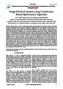
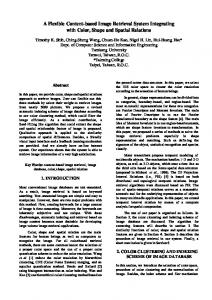
2 System Overviews The architecture of the content-based image retrieval system for real images as shown in Figure 1 is described as follows. In the offline phase, a training image is segmented and the main object is detected first. Then, five feature descriptors such as color, texture, and shape defined in the MPEG7 specification are extracted from the training image; i.e., ColorLayout descriptor, ColorStructure descriptor, EdgeHistgram descriptor, HomogeneousTexture descriptor, and RegionShape descriptor, totally 221 dimensions. As we know, the features extracted from images play an important role in image classification. If the relevant features for classification are deliberately selected, images would be easily distinguished based on them. Here, a meta-heuristic optimization algorithm called Self-Adaptive Harmony Search (i.e., SAHS) algorithm is used to select the features for a corresponding image category. Then, Support Vector Machine (SVM) is used as the classifier to detect an image category. In training SVM, two approaches are proposed to build SVM classifiers as shown in Figure 2. The first one is “One-against-all” where a classifier for each category is trained to distinguish a query image. For N classes (or categories), there would be N binary classifiers. The second one is “One-against-one” where a classifier for each possible pair of classes is trained. For N classes, there would be N(N-1)/2 classifiers. For this approach, since much more classifiers should be trained for a large number of classes, a densitybased clustering process is done first to reduce the number of classes (i.e., from N to n). Besides, we also build MPEG-7 signatures using K-means clustering on all images to accelerate image retrieval.
Offline Phase
Training Images
Segmentation and Main Object Detection
Feature Extraction
K-means Clustering
Feature Selection Using SAHS Image Database Training SVM
Signatures
Online Phase
Query Images
Segmentation and Main Object Detection
Feature Extraction
SVM Classification
Majority Voting Strategy
Similarity Measure
Result Images
Figure 1 System architecture Training SVM
One-Against-All SVM1
SVMN
Image Features
One-Against-One SVM1(1,2)
SVM1,2
DensityBased Clustering
SVM1(1,3)
n clusters
SVMn −1,n SVMn (i,j)
Figure 2 Training SVM
In the online phase, we also do the same processing on a query image, including segmentation, main object detection, and feature extraction as mentioned. Then, we find out 1) the images in the predicted class of the query image as the first candidates, based on the majority voting strategy, and 2) the images with the same MPEG-7 signatures as the query image as the second candidates. Finally, we get the images which appear in both groups of candidates, and rank them according to the similarity measure.
3 Preprocessing In the preprocessing, an image is segmented and the main object is detected first. Then, five feature descriptors such as color, texture, and shape defined in the MPEG7 specification are extracted from the image, totally 221 dimensions. Finally, relevant features are selected for facilitating image classification, using the SAHS algorithm.
3.1. Segmentation and Main Object Detection In the real world, an image is usually composed of several objects with different colors, textures, and shapes. In general, the existing CBIR methods extract features either from a whole image [2, 25, 26, 29] or from a segmented image for further processing [16]. Since there could be undefined or ambiguous regions in an image, a classifier cannot be accurate enough when extracting features from a whole image. Therefore, extracting only the highlight of an image (or the main object of an image) is essential to improve classification accuracy. Here, an image method called JSEG [21] is used to segment the objects in an image. The JSEG method consists of two steps, color space quantization and spatial segmentation. First, JSEG quantizes colors of an image into several representative classes. Then, it labels pixels with the color classes to form a class map of the image. Finally, the image is segmented using multi-scale J-images. The segmentation result of an image using JSEG is shown in Figure 3.
Figure 3: (a) Original image (b) Segmentation result using JSEG
As shown in Figure 3, the segmentation result is appropriate for background objects, but the main object in the image is over-segmented; as a result, the features extracted from these over-segments are not specific to represent the main object. In order to enable deriving the main object, the Snake algorithm facilitating the detection is used. The Snake algorithm known as an Active Contour Model (ACM) was proposed by Kass et al. [17] and widely used in medical image analyses and two-dimensional image contour detection. While applying ACM, an initial contour for the image object and iteration time is set. The edge of the initial contour is dynamically altered by modifying an energy function. Finally, the contour converges gradually to the real edge of the object in an image. In fact, the contour alteration would stop until minimizing the energy function or reaching specified iteration time.
The revised ACM algorithm proposed by Lankton and Tannenbaum [19] is adopted in this paper. The well-known defect of ACM is the time consuming problem, so the sparse field method (SFM) proposed by Whitaker [31] is used to improve the efficiency [20]. Owing to the variety of background color images, the contour of the main object cannot reach the best convergence if the image has complex background energies; therefore, we combine JSEG with ACM to detect the main object. The combination method is shown in Figure 4 where α is a threshold in the range [0, 1].
for each segment i-seg after using JSEG if (|i-seg pixels|∩active contour track) > |i-seg pixels|×α i-seg becomes one part of the main object end end
Figure 4: Main object detection method
Here, ACM is used to facilitate JSEG and the method determines which segments should become parts of the main object. If the intersection of a segment and the active contour is larger than α times size of the segment, then the segment becomes a part of the main object. As shown in Figure 5(a), we set an initial contour for the main object to be the middle sixteen macro blocks, and the iteration time is 2000 units. After applying ACM, the background of the image is still not eliminated very well as shown in Figure 5(c). Then, we use the main object detection method given above and merge the chosen segments together; finally, the main object is detected as shown in Figure 5(d).
Figure 5: (a) Initial contour, (b) Result contour of the ACM algorithm, (c) Result contour with color images (d) Detected main object
3.2. Feature Extraction In this paper, we adopt the bag-of-features MPEG-7 [1, 2, 3, 4, 13, 14, 22, 23, 24] defined by the MPEG organization, which consists of color description (i.e., two color descriptors), texture description (i.e., two texture descriptors), and shape description (i.e., one shape descriptor). Among them, the descriptors relevant to image characteristics are as follows and the numbers of their features are shown in Table 1. 1. 2. 3. 4. 5.
ColorLayout Descriptor describes the layout and variation of colors and this reflects the color combinations in an image. ColorStructure Descriptor counts the contents and structure of colors in an image by using a sliding window. EdgeHistogram Descriptor counts the number of edge occurrences in five different directions in an image. HomogeneousTexture Descriptor calculates the energies of an image in the frequency space, which are the level of gray-scale uniform distribution and texture thickness, and this reflects the texture characteristics in an image. RegionShape Descriptor relates to the spatial arrangement of points (pixels) belonging to an object or a region in an image. Descriptor ColorLayout ColorStructure EdgeHistogram HomogeneousTexture RegionShape Total
Number of Features 12 32 80 62 35 221
Table 1: Descriptor features
3.2.1. ColorLayout Descriptor (CLD) To extract CLD features, an image on the RGB color space is partitioned into 8*8=64 blocks first; then, the average color of each block is calculated and converted into YCbCr color; next, each Y, Cb, Cr color space is transformed by 8x8 DCT, so that three sets of 64 DCT coefficients are obtained; finally, a zigzag scanning is performed with these three sets of 64 DCT coefficients, and CLD features are extracted with the specified length 12 (i.e., 6 coefficients from Y, 3 coefficients from Cb, and 3 coefficients from Cr).
3.2.2. ColorStructure Descriptor (CSD) A statistical way is used to get the contents and structure of colors in an image in the global and local space. First, the color space of an image is converted into the HMMD color space represented with (hue, max, min). Then, an 8*8 structuring element is used to count color structure histogram. For two images, if their colors are the same and the numbers of pixels are also the same, but their color distributed structures are different, the color structure histogram would be different.
3.2.3. EdgeHistogram Descriptor (EHD) EHD presents the line characteristics with 5 directions in the local area of an image. Here, an image is divided into 4*4=16 sub-images and each sub-image is represented by 5 different directional edges (or by 5-bin edge histogram). Thus, an entire image consists of 16*5=80 EHD features.
3.2.4. HomogeneousTexture Descriptor (HTD) In the homogeneous texture description, energy and energy deviation can be used to describe the regional texture features. HTD is represented based on the frequency space which is divided into 6 parts by 30 degrees and then is cut into 5 parts on a radius using the octave division. Thus, totally 30 frequency subspaces called feature channels are generated. Finally, the sum of squares and the standard deviation of the image intensity form energy and energy deviation, respectively in each channel. Including the entire space, HTD has 62 8-bit values. The energy here reflects the texture characteristics in an image; in other words, if an image has large energy, the texture variance is relatively large.
3.2.5. RegionShape Descriptor(RSD) Shape features relate to the spatial arrangement of points (pixels) belonging to an object or a region. They provide a strong clue to object identity and functionality, and can even be used for object recognition. Many applications including those concerned with visual object retrieval or indexing use shape features. Here, we use RSD to express the pixel distribution within a 2-D object region. It can describe complex objects consisting of multiple disconnected regions as well as simple objects with or without holes. The default RSD has 140 bits and uses 35 coefficients quantized to 4 bits/coefficient to represent the shape features.
3.3. Feature Selection Using SAHS The purpose of feature selection is to select the most relevant features to facilitate the classification. Feature selection algorithms could be categorized into three different approaches: wrapper, filter, and embedded. The wrapper approach utilizes the performance of a target classifier to evaluate feature subsets; it is computationally heavy since a target classifier must be iteratively trained on each feature subset. The filter approach evaluates the performance of feature subsets through an independent filter model before a target classifier is applied. The embedded approach must utilize a specific classification algorithm containing the evaluation body inside. Here, we use the filter approach to select the most relevant features since its computational loading is acceptable and the selected classification algorithm could not be specific. In our work, the feature selection model consists of two parts: Self-Adaptive Harmony Search (i.e., SAHS) algorithm [12] and relative correlations [27], as illustrated in Figure 6. Once the original feature set is given, the SAHS algorithm starts to iteratively search a better solution that would be evaluated later by the relative correlations. Finally, the best solution will be output as the final feature subset. Feature Selection Model SAHS Original Feature Set
Final Feature Subset relative correlations
Figure 6: Feature selection model
4 Methods In the offline phase, SVM classifiers are trained using the relevant features selected by SAHS. Next, the MPEG-7 signatures of all images are generated using K-means clustering. Finally, in the online phase, we find out result images most similar to a query image after the similarity measure.
4.1. Training SVM In this paper, two approaches are proposed to build SVM classifiers. The first one is “one-againstall” where a classifier for each category is trained to distinguish a query image. For N classes (or categories), there would be N binary classifiers. The second one is “one-against-one” where a classifier for each possible pair of classes is trained. For N classes, there would be N(N-1)/2 binary classifiers. For the second approach, when there are a large number of classes, a density-based clustering process is done first and then the first-level classifiers for each pair of clusters are trained. Next, the secondlevel classifiers for each pair of classes in a cluster are trained. If 30 classes are clustered uniformly into 3 groups, we need to train the classifiers of 3 clusters and the classifiers of 10 classes in each cluster. Thus, the number of trained classifiers can be reduced from (30 × 29/2) = 435 to (3 × 2/2) + (10 × 9/2) × 3 = 138. Rather than using K-means to cluster all the images because of requiring to specify the exact cluster number, Density-Based Spatial Clustering of Applications with Noise (DBSCAN) is used here. Furthermore, DBSCAN can confront noises and process any shape and size of clusters, so that it can find the clusters which K-means cannot find. However, DBSCAN needs to set two parameters eps and MinPts. Parameter eps specifies how close points should be to each other and are considered as parts of a cluster. Parameter MinPts specifies the minimum number of neighbors that should be included in a cluster. If eps is set extremely large, all points will be clustered into one single cluster whereas it is set too small, the number of clusters becomes much more. On the other hand, if MinPts is set too large, most points are treated as noise points. To obtain the optimal parameters eps and MinPts, eps = [10, 20, … 1000] and MinPts = [10, 20, … 1000] , totally 100 × 100 = 10000 combinations are tested in the experiments. For DBSCAN, points can be classified into 3 types; i.e, core points, (density-) reachable points, and outliers defined as follows. 1.
Core point: a core point means that the number of nearby points exceeds the certain threshold in a neighborhood range, and it is a part of a cluster.
2.
Reachable point: a point is reachable from a core point, but the number of nearby points does not exceed the certain threshold in a neighborhood range.
3.
Outlier: an outlier is a noise point that is neither a core point nor a reachable point.
In short, the size of the neighborhood is determined by parameter eps, and the density (or threshold) is determined by parameter MinPts. For the example with MinPts=3 as shown in Figure 7, core points form a cluster together where all inside points are reachable from themselves. Each cluster contains at least one core point. Although reachable points can be parts of a cluster, they merely form the “edge” of a cluster because they cannot be used to reach more points.
Figure 7: Density clustering (red) core points, (yellow) reachable points, (blue) outliers
4.2. MPEG-7 Signatures Based on K-means Clustering For each extracted visual descriptor, K-means is used to partition it into two clusters respectively, and mark them 0 and 1. Then, we combine the cluster numbers from the five visual descriptors together and obtain a 5-digit MPEG-7 signature as shown in Table 2. Thus, an MPEG-7 signature can represent the characteristics of an image. An MPEG-7 signature has 5 digits with 2 different values each, so that (2) = 32 bins could be used to distinguish the characteristics of images. Since K-means compresses images into clusters, we are able to build an index structure more easily using these signatures. Besides, the centroids of K-means on the five visual descriptors are also stored for the similarity measure in the online phase. Visual Descriptor
CL
CS
EH
HT
RS
Cluster Number
1
0
1
1
1
The signature is 10111 Table 2: MPEG-7 signatures
4.3. Similarity Measure First, we extract the MPEG-7 visual features from a query image. Then, we find out the images in the predicted class of the query image as the first candidates, based on the majority voting strategy. Next, the similarity measure between the visual features extracted from the query image and the recorded centroids of K-means on the five visual descriptors is performed to determine cluster numbers, respectively. The cluster numbers of the most similar centroids are combined together to become the query signature. Then, we can find out the images with the same MPEG-7 signature as the query image as the second candidates. Finally, we get the images which appear in both groups of candidates, and rank them according to the Euclidean distances from the query image.
5 Implementation We have implemented an “Image Search Engine” system to search the similar images to a query image from an image database, based on the proposed techniques. First, two datasets Corel and Nature used to evaluate the state-of-the-art methods and ours are described. The experiments were implemented in C# and conducted on an Intel Core 2.93GHz, 4GB RAM with Windows 7. The well-known LIBSVM developed by Chang and Lin [4] was adopted as an SVM classifier in the experiments. Finally, experiment results are presented to show the superiority of our method over the other methods.
5.1. Datasets First, to evaluate our method and compare with the state-of-the-art methods, 10 classes of the Corel dataset are selected and tested in the experiments. Totally, there are 1000 general-use images in the image database and each class has 100 images on the same topic namely, Africans, Beaches, Buildings, Buses, Dinosaurs, Elephants, Flowers, Food, Horses, and Mountains, as shown in Figure 8. The size of each image is either 256 × 384 or 384 × 256.
Figure 8: Ten classes of the Corel dataset
Furthermore, to evaluate our method comprehensively, the dataset called Natural is manually collected from Flickr, totally 30 classes; i.e., Airplane, Bicycle, Bird, Butterfly, Car, Cat, Chicken, Clock, Cow, Deer, Dog, Dolphin, Elephant, Flower, Giraffe, Hedgehog, Horse, Lion, Moon, Motorcycle, Panda, Pig, Rabbit, Sakura, Ship, Snake, Spider, Tiger, Train and Turtle. Totally, 7384 random-size images are collected in the image database and each class has at least 200 images.
5.2. Experiment Results 5.2.1. Comparisons with the Other Methods In this experiment, we compare the proposed method with the other methods using the same Corel dataset where each image is taken as a query image. If a retrieved image is with the same class as that of the query image, it is considered successful; otherwise it fails. Here, the precision is used as a performance measure as follows. Precision =
Number of Relevant Images Number of Relevant Images + Number of Irrelevant Images
Liberal, normal, and strict represent the classification degree of LIBSVM. For the liberal, we select all predicted classes in the one-against-all and one-against-one approaches as the first candidates; for the normal, half predicted classes with higher probabilities in the one-against-all approach (or half predicted classes in the one-against-one approach) are as the first candidates; for the strict, the predicted class with the highest probability in the one-against-all approach (or one of predicted classes in the oneagainst-one approach) is as the first candidate. The experimental results and comparisons are shown in Table 3. Regardless of what approaches are used, our method always performs much better than the other methods.
One-against-all One-against-one
Liberal Normal Strict Liberal Normal Strict
Other methods
10 classes 74.41% 87.37% 92.6% 95.93% 96.12% 96.3% 55% [18] 67.16% [28]
9 classes 78.71% 89.44% 91.66% 96.13% 96.12% 96.33% 75% [6]
6 classes 86.51% 93.86% 94.83% 95.11% 95.23% 95.16% 79% [15] 86% (feedback) [15]
5 classes 94.23% 98.14% 98.2% 99.18% 99.08% 99% 72% [5]
Table 3: Comparisons with the other methods
In general, the less the class number to be classified, the better the performance of a method. However, it seems not true for the one-against-one approach since the precision of 9 classes is better than those of 6 classes. The reason is that some classes with better performances are removed from 9 classes, as shown in Table 4. Beaches Buildings Buses Dinosaurs Elephants Flowers Food Horse Mountains
9 classes 84.85% 90.6% 97.4% 99% 98.7% 98.3% 97.4% 100% 99%
6 classes 85.8% 90.7% 99% 98.6% 99% 97.6%
Table 4: Classification precision
5.2.2. Experiments on Extensive Functionality In this experiment, our method is evaluated comprehensively using the dataset Natural with 30 classes. Here, two kinds of query images are used to test the system performances; one is within the dataset, and another is outside the dataset. For query images within the dataset, 200 images for each class are taken as query images, and the precision is shown in Table 5. The one-against-one approach presents better results than the one-against-all approach for the case of without checking the class of the most similar image. Since the most similar image is indeed the query image, we can further improve the precision by retrieving the images with the same class as the query image, and make the precision reach 100%.
30 classes One-against-all One-against-one
Liberal Normal Strict Liberal Normal Strict
33.88% 40.51% 54.11% 74.71% 74.88% 74.85%
30 classes (after checking) 100% 100% 100% 100% 100% 100%
Table 5: Precision of query images within the dataset
For query images outside the dataset, 10 images for each class are taken from Flicker as query images, and the precision is shown in Table 6. Similarly, the one-against-one approach still performs better than the one-against-all approach. Here, we can use the “Feedback” button to improve the precision by clicking relevant images. Although the one-against-all approach has worse precision, it finds more possible classes, and this makes the feedback function reveal its benefit. 30 classes One-against-all One-against-one
Liberal Normal Strict Liberal Normal Strict
21.19% 24.50% 34.33% 42.8% 43.45% 43.33%
30 classes (after feedback) 76.66% 63% 34.33% 47.33% 44% 43.33%
Table 6: Precision of query images outside the dataset
6 Conclusions In this paper, an image search engine system for real images is proposed and implemented to search the similar images to a query image from an image database. First, we segment out the main object in an image and then extract its features. Totally, 221 visual features are extracted from the main object. In general, a classifier trained by the object-based feature vectors is more precise than that trained by the feature vectors from a whole image. Next, relevant features are selected from the original feature set for facilitating image classification, using the SAHS algorithm. Then, two approaches “one-againstall” and “one-against-one” are proposed to build SVM classifiers trained using the relevant features selected by SAHS. Furthermore, the MPEG-7 signatures of all images are generated using K-means clustering. In the online processing, the result images most similar to a query image can be found after the similarity measure. Finally, the experimental results show that our method is feasible in image searching from the real image database and more effective than the other methods.
References [1] M. Bober, “MPEG-7 visual shape descriptors,” IEEE Transactions on Circuits and Systems for Video Technology, Vol. 11, No. 6, pp. 716-719, 2001. [2] R. Brown and B. Pham, “Image mining and retrieval using hierarchical support vector machine,” Proc. the International Conference on Multimedia Modeling, pp. 446-451, 2005.
[3] S. F. Chang, T. Sikora, and A. Puri, “Overview of the MPEG-7 standard,” IEEE Transactions on Circuits and Systems for Video Technology, Vol. 11, No. 6, pp. 688-695, 2001. [4] C. C. Chang and C. J. Lin, “LIBSVM: a library for support vector machines,” ACM Transactions on Intelligent Systems and Technology, Vol. 2, No. 3, pp. 27:1-27:27, 2011, software available at http://www.csie.ntu.edu.tw/~cjlin/libsvm. [5] R. Chaudhari and A. M. Patil, “Content based image retrieval using color and shape features,” International Journal of Advanced Research in Electrical, Electronics and instrumentation Engineering, Vol. 1, No. 5, pp. 386-392, 2012. [6] R. Choudhary, N. Raina, N. Chaudhary, R. Chauhan, and R. H. Goudar, “An integrated approach to content based image retrieval,” Proc. International Conference on Advances in Computing, Communications and Informatics, pp. 2404-2410, 2014. [7] W. S. Chow and M. K. M. Rahman, “A new image classification technique using tree-structured regional features,” Neurocomputing, Vol. 70, No. 4-6, pp. 1040-1050, 2007. [8] Y. Deng and B. S. Manjunath, “Unsupervised segmentation of color texture regions in images and video,” IEEE Transactions of Pattern Analysis and Machine Intelligence, Vol. 23, No. 8, pp. 800810, 2001. [9] M. K. Hasan, L. Chen, and C. G. Brown, “Image data mining and classification with DTree ensembles for linguistic tagging,” Proc. the IEEE Workshop on Computational Intelligence for Visual Intelligence, pp. 29-36, 2009. [10] Y. F. Huang and H. Y. Lu, “Automatic image annotation using multi-object identification,” Proc. the 4th Pacific-Rim Symposium on Image and Video Technology, pp. 386-392, 2010. [11] Y. F. Huang and H. W. Chen, “A multi-type indexing CBVR system constructed with MPEG7 visual features,” Proc. the International Conference on Active Media Technology, Lecture Notes in Computer Science, Vol. 6890, pp. 71-82, 2011. [12] Y. F. Huang and C. T. Wang, “Classification of painting genres based on feature selection,” Proc. the 8th FTRA International Conference on Multimedia and Ubiquitous Engineering, pp. 159164, 2013. [13] Y. F. Huang and S. M. Lin, “Searching images in a textile image database,” Proc. the 5th International Conference on Swarm Intelligence, pp. 267-274, 2014. [14] ISO/IEC 15938-3, Information Technology – Multimedia Content Description Interface-Part3: Visual, 2002. [15] MS. R. Janani and S. K. Palaniappan, “An improved CBIR method using color and texture properties with relevance feedback,” International Journal of Innovative Research in Computer and Communication Engineering, Vol. 2, Special No. 1, pp. 47-56, 2014. [16] P. Kalva, F. Enembreck, and A. Koerich, “WEB image classification based on the fusion of image and text classifiers,” Proc. the Ninth International Conference on Document Analysis and Recognition, Vol. 1, pp. 561-568, 2007. [17] M. Kass, A. Witkin, and D. Terzopoulos, "Snakes: active contour models," International Journal of Computer Vision, Vol. 1, No. 4, pp. 321-331, 1987. [18] G. Khosla, N. Rajpal, and J. Singh, “Evaluation of Euclidean and Manhanttan metrics in content based image retrieval system,” International Journal of Engineering Research and Applications, Vol. 4, No. 9, pp. 43-49, 2014. [19] S. Lankton and A. Tannenbaum, “Localizing region based active contours,” IEEE Transactions on Image Processing, Vol. 17, No. 11, pp. 2029-2039, 2008. [20] S. Lankton, “Sparse field methods,” Technical Report, Georgia Institute of Technology, 2009. [21] H. Lu, Y. B. Zheng, X. Y. Xue, and Y. J. Zhang, “Content and context-based multi-label image annotation,” Proc. the IEEE Conference on Computer Vision and Pattern Recognition, pp. 61-68, 2009.
[22] B. S. Manjunath, J. R. Ohm, V. V. Vasudevan, and A. Yamada, “Color and texture descriptors,” IEEE Transactions on Circuits and Systems for Video Technology, Vol. 11, No. 6, pp. 703-715, 2001. [23] J. M. Martinez, R. Koenen, and F. Pereira, “MPEG-7: the generic multimedia content description standard, part 1,” IEEE Multimedia, Vol. 9, No. 2, pp. 78-87, 2002. [24] J. M. Martinez, “MPEG-7 overview (version 10),” ISO/IEC JTC1/SC29/WG11 N6828, 2004. [25] H. Pourghassem and H. Ghassemian, “Content-based medical image classification using a new hierarchical merging scheme,” Computerized Medical Imaging and Graphics, Vol. 32, No. 8, pp. 651-661, 2008. [26] J. L. Shen, “Stochastic modeling western paintings for effective classification,” Pattern Recognition, Vol. 42, No. 2, pp. 293-301, 2009. [27] G. Silviu, Information Theory with Applications, McGraw-Hill, 1977. [28] P. Srivastava, O. Prakash, and A. Khare, “Content-based image retrieval using moments of wavelet transform,” Proc. the International Conference on Control, Automation and Information Sciences, pp. 159-164, 2014. [29] C. F. Tsai, “Image mining by spectral features: a case study of scenery image classification,” Expert Systems with Applications, Vol. 32, No. 1, pp. 135-142, 2007. [30] V. S. M. Tseng, M. H. Wang, and J. H. Su, “A new method for image classification by using multilevel association rules,” Proc. the 21st International Conference on Data Engineering Workshops, pp. 1180-1180, 2005. [31] R. Whitaker, “A level-set approach to 3D reconstruction from range data,” International Journal of Computer Vision, Vol. 29, No. 3, pp. 203-231, 1998.