A system to analyze social media data to understand events in described in ... done using TweetCollector, a twitter data management system that developed by ...
Content-based prediction of temporal boundaries for events in Twitter Akshaya Iyengar, Tim Finin and Anupam Joshi Department of Computer Science and Electrical Engineering University of Maryland, Baltimore County Baltimore, Maryland 21250 email: {akshaya1,finin,joshi}@umbc.edu
Abstract—Social media services like Twitter, Flickr and YouTube publish high volumes of user generated content as a major event occurs, making them a potential data source for event analysis. The large volume and noisy content of social media makes automatic preprocessing essential. Intuitively, the eventrelated data falls into three major phases: the buildup to the event, the event itself, and the post-event effects and repercussions. We describe an approach to automatically determine when an anticipated event started and ended by analyzing the content of tweets using an SVM classifier and hidden Markov model. We evaluate our performance by predicting event boundaries on Twitter data for a set of events in the domains of sports, weather and social activities.
I. I NTRODUCTION The increased use of social media websites like Twitter has created vast amounts of content generated by people from different countries and diverse backgrounds. Due to its broad reach, Twitter has been effectively used not only for commercial purposes but also for social causes. The power of this medium was seen during the 2011 Egyptian protests where it was one of the primary modes of communication for both participants and organizers of the protest. The popularity and dynamic nature of Twitter allows us to chronicle events in real-time. In many cases the tweets are by users who are participating in or immediately affected by the event. For events that transpire over time and space, such as the dispersal of an oil spill, a hurricane or a spreading wildfire, we can use this data to analyze how the event progressed, traveled geographically and identify its major sub-events. We can also study the reactions of people to disaster relief efforts. For such analysis, due to the large volume of tweets, automatically categorizing the information into temporal classes is an important preprocessing step. Our goal is to automatically determine when an event starts and when it ends, segmenting the event-related data into three major phases: the buildup to the event, the event itself, and the post-event effects and repercussions. In this study, we have focused on what we can learn by analyzing the content of the tweets about the event. The message volume also provides an important and valuable signal, but is largely independent of the content signal, which is the focus of this study. Future work will combine content, volume and context features for the event segmentation task.
We present a system that classify event data into temporal classes and then uses a hidden Markov model and other methods to predict event boundaries. We identify key challenges that arise due to the noisy nature of data on Twitter and similar social media systems. II. BACKGROUND AND R ELATED W ORK In this research, we analyze the data, not only during an event but also before and after it. Most of the current research has been in detecting events by continuously monitoring the Twitter data stream. To our knowledge, this is the first research on detecting temporal boundaries from content for anticipated events like sports games, public events and weather events in large pre-collected datasets. Since approach uses only the content of tweets and does not depend on volume information, it is applicable when accurate estimates of volume are not readily available. There has been some research on detecting and analyzing events on Twitter. Shamma et al. [1] analyzed the Twitter time line to identify the structure of broadcast events. Event summarization using HMMs to provide better search results is described by Chakrabarti et al. [2]. Sakaki et al. [3] detect a target event in Twitter using Kalman filter and particle filters. A system to analyze social media data to understand events in described in Sheth et al. [4]. Early work by Java et al. described techniques to automatically classify a person’s intent in publishing a tweet [5]. The use of social media in disaster events and emergency response has also been studied by several groups [6]–[8]. III. DATA C OLLECTION AND L ABELING We applied our techniques on multiple events from different domains, including sports (e.g., football and cricket), weather (e.g., hurricane) and social events (e.g., the 2011 UK royal wedding). The data collection, storage and preprocessing was done using TweetCollector, a twitter data management system that developed by our research group. The gold standard training data for each event was annotated by hand to identify the temporal boundaries. Individual tweets were treated as data instances which were ordered by their timestamp and labeled as either before, during or after. Table I shows some sample of labeled tweets from the SuperBowl XLV dataset. It is observed that for many events, close to
TABLE I S AMPLE TWEETS FROM S UPER B OWL DATASET WITH CLASS LABELS Label Before
During
After
Tweets Guess ima hop in the shower and stay home for the superbowl... Go Packers ! Best wishes to all the supporters in Spring Green WItonight. http://bit.ly/aYyj6O Touch Down Packers Booooooooooom!!7-0 :’( 49 secs left and the packers are winning. #nobueno Packers won #superbowl http://myloc.me/htWYp PACKERS!!! yay! Steelers lost!!! TABLE II
N UMBER OF TWEETS IN EVERY CLASS BY EVENT Event Superbowl XLV India v Australia CWC India v Pakistan CWC India v Sri Lanka CWC Royal Wedding Hurricane Igor
Before 3863 2792 11393 7571 3413 4547
During 3893 2615 13732 10464 5275 5124
After 3889 3310 10444 9952 4238 4768
Total 11645 8717 35569 27987 12926 14439
the transition points, it is hard to identify a single accurate separation point. Due to space constraints, details of how we resolve this issue, can be found in [9]. Additionally, there are many tweets which cannot be classified into either of the classes, merely by looking at the content alone. Some of the causes for this may be because they do not contain any temporal indicators or because they are spam. Since we would always find such instances in the real world data stream, we believe it is important that our system performs well despite being given such noisy data. Hence we assign classes to them as well. An alternative would be to ignore tweets containing no temporal information. After deciding the event boundaries on the entire data for a particular event, we sample the data to get reasonably sized dataset with fairly balanced classes . All samplings were done while maintaining the chronological order of the tweets. Thus if we reduce the dataset to one-tenth, we do so by taking every tenth instance in a bucket. Table II shows details of the some of our datasets. IV. A PPROACH AND S YSTEM A RCHITECTURE In order to estimate temporal boundaries, our aim is to learn from the datasets, the general features that are most indicative of the time of occurrence of a tweet relative to the event. We explored possible features like bag-of-words and verb phrases. We trained a multi-class support vector machine (SVM) to classify the event data into the three temporal buckets and used different algorithms to estimate the boundaries. Figure 1 shows our high level system architecture. The following sections give a brief overview of each component of our system. A. Feature Generation Once the datasets were labeled, we converted each data instance into a feature vector containing feature number and value. The feature number is fixed for the entire dataset. Due to large number of null valued features, we used a sparse feature
Fig. 1. We use supervised learning to construct a classifier that predicts whether a tweet occurs before, during or after an event. The final event boundaries are determined by analyzing the tweet stream using a simple local error-minimization algorithm or a hidden Markov model.
vector (SFV) where all the null values are assumed implicitly. The following sections discuss the features we used and how their values were calculated. Bag of Words. Bag of words (BOW) is a very commonly used feature. In this method, each instance is treated as group of words. We build an index of all words seen in the dataset. Every word has a unique id which is also used as a feature number. A word count is calculated for every word present in a tweet. Every word from the unigram index, not present in the current instance gets a zero value. For the experiments discussed in this paper, we consider only unigram features. Before splitting the tweets into words, we get rid of URLs, retweet symbols (denoted by RT) and user mentions (starting with @user-name) as these are not words. We keep hashtags (denoted by #mytag) as they are a valuable feature and are query terms in many cases. Presently we are not dealing with punctuation in any special way. The Twitter data is extremely noisy. Users use many abbreviations, both standard and ad hoc, to accommodate the short message length. The informality of the genre results in the common use of special characters and terms (e.g., URLs, hashtags, emoticons) and the presence of many uncorrected errors in spelling and grammar. The following examples of tweets from the cricket datasets demonstrates the need for specialized parsers that can handle the noise that is typical of user generated content on social media websites. Watchin cricket is sooooo borin http://bit.ly/aYyj6O ... & I.N.D.I.A. is in F.I.N.A.L.S. for Cricket World Cup 2011 - against Sri Lanka, a strong team indeed. Looking forward to Saturday. RT @Mariyaaa H Yeh it is :( even am watchin #cricket dis time its quite intrestin u kno lmfao
Verb-based Features. When human annotators determine which class, before, during or after an event, a given instance belongs to, we look at the tense of the sentence relative to the event. The verb phrases used in a sentence and their types, are an important indicator of the tense of the sentence. We use this idea to generate verb-based features using a two step process. 1) Identifying verbs. We first annotate each instance with its part-of-speech (POS) tags using the pre-trained
TABLE III A SUBSET OF THE P ENN T REEBANK POS TAGS FOR VERBS Tag MD VB VBD VBG VBN VBP VBZ
Description Modal Verb, base form Verb, past tense Verb, gerund or present participle Verb, past participle Verb, non-3rd person singular present Verb, 3rd person singular present
left3words-wsj-0-18 model from the Stanford Log-linear POS Tagger [10]. This tagger uses the Penn Treebank Tagset (PTB) discussed in [11]. AN example of the tagged output is: the/DT doctor/NN is/VBZ examining/VBG the/DT effects/NNS that/WDT the/DT treatment/NN has/VBZ on/IN the/DT patient/NN ./. 2) Identify verb tag phrase. We identify any sequence of verbs in terms of their tag phrases. Table III shows the subset of the tags from [11] that have been used for our verb features. In the above example we have two such phrases: VBZ VBG (is examining) and VBZ (has). We experimentally chose 36 verb features as described in the sections below. Grammatically correct Verb Features. In order to identify the commonly occurring verb phrases, we created a set of grammatically correct sentences encompassing all the different kinds of tenses occurring in the language. For each of the three tenses Present, Past and Future, we used sample sentences from the simple, perfect, progressive and perfect progressive tenses. We found a total of 18 unique verb tag phrases across all the tenses. We then tagged a test set of grammatically correct sentences and found that these 18 tag phrases accounted for all the verb phrases occurring in the test set. Hence we treat these as our “gold standard” verb features. Verb Features from Twitter. Twitter status updates often consist of sentence fragments or otherwise ungrammatical sequences and are rife with mis-spellings, odd abbreviations, URLs, hashtags and other non-word terms. Moreover, the standard conventions for capitalization and punctuation are not followed. As a result, there are common phrases occurring in tweets which are consistently mis-tagged by the Stanford POS Tagger, which was trained on well formed text from Wall Street Journal articles [10]. To overcome this, we find additional verb tag phrases occurring in the our datasets. We apply the tagger on a dataset created by combining tweets from events mentioned in Table II to select 18 verb phrases that each occur more than 50 times. Calculating Feature Values. For the bag-of-words features, we use unigram id as feature number and word count in an instance as feature value . However since we rarely found a verb phrase occurring multiple times in an instance, for the verb feature we use a boolean value of 1 or 0 depending on whether the verb phrase occurred in the instance. go packers ! bep was lame at 1/2 time.
TABLE IV C LASSIFICATION ACCURACIES WITH DIFFERENT FEATURE SETS Dataset Superbowl XLV India v Australia CWC India v Pakistan CWC India v Sri Lanka CWC Royal Wedding Hurricane Igor
BOW 62.02% 72.79% 66.57% 70.87% 55.29% 71.62%
BOW+gold 61.85% 72.69% 66.48% 70.80% 55.34% 71.55%
BOW+all 61.62% 72.91% 66.52% 71.00% 56.16% 71.58%
1:1 2:1 77:1 166:1 178:1 310:1 665:1 3897:1 4952:1 6304:1 17704:1
B. Training Classifiers After converting the datasets into SFV format, we used this data to train models that can classify a given tweet into one of our three classes: before, during or after. Since there are three classes, we use the multiclass support vector machine provided in SVM Light [12]. A separate SVM for each of the seven datasets mentioned in Table II. We evaluate accuracies for different values of parameter C, which is the tradeoff between training error and margin. Increasing C increases the complexity of the model allowing it to handle more complex datasets. After trying values of C from 1 to 100,000, we empirically determined 30,000 to be a good value. We performed a ten fold cross-validation for each event dataset. Since we are dealing with temporal aspect of data, all our datasets are chronologically ordered by their time stamp. We want to maintain this relative ordering or data through the entire process. Hence we do not shuffle out data while making the split. For dividing into ten folds, we put every 10th instance in the same bucket. We use the accuracies of each fold to calculate the total accuracy of the system. We then combine all the ten test folds back into the original order before the split. Thus for each dataset we get a new predicted class labels for all instances. For evaluating the usefulness of the different features we built models using three groups of features: bag of words, bag of words and “gold verbs”, and bag of words and all verbs. We found that the verb features did not provide any significant boost to accuracy as seen in Table IV. This may be due to the noisy data and we intend to use Twitter specific POS taggers in the future [13]. Hence, in this paper we present results obtained using only the bag-of-words feature for all further experiments. Detailed experimental results using all the feature sets have been provided in [9]. We believe that our analysis of verbs and their potential use as features is a small step in the direction. We could add more features that are specific to a domain like sports (e.g., wins, lost, playing) that give temporal clues about a tweet. We could also use temporal terms (e.g., tonight, tomorrow, today, now, later) in conjunction with the verbs and use their presence as features in the future. Improving Accuracy using Sliding Windows. We further improve the classifier accuracy by using a sliding window approach. In this case we take a window of a fixed size and slide it over our sequence of predicted class labels. A
Fig. 2. Classification accuracy is improved by computing a simple “moving average” that labels each tweet with the most common class within a window around it.
window of size X around a data instance consists of X/2 instances on both its sides. For each data instance we take a majority vote of class labels in the window and modify its class label accordingly. This gives us a smoothing over the data by using the density of predicted labels. Figure 2 shows the improvement in accuracies observed. We have tried smoothing with window of different sizes in {1, 10, 20, 30, 50, 100}. We notice that for each dataset, the accuracy keeps on increasing significantly till window size 20. After that the boost in accuracy is low. For window sizes 30, 50 and 100 the difference is less than 1% in most cases. Even though the number of labels modified increases it does not cause a significant improvement in the accuracy. Hence we determined that window sizes of 30 and 50 were reasonable for all our further experiments. C. Estimating Temporal Boundaries The use of sliding windows discussed in previous section improved our classification accuracies significantly. Once we get the predicted class labels for the dataset, we develop a technique to draw the two event boundaries while minimizing the error. We calculate error for each of the two boundaries separately. Error is calculated as the sum of proportion of misclassified instances. We place each boundary where its classification error as described above is minimum. We evaluated two approaches: a simple local error minimization algorithm applied independently to the two boundaries and a hidden Markov model applied to the entire stream. The Cuts Algorithm. Our data consists of three classes, before, during and after, encoded as 1, 2 or 3. Our classifier combined with the sliding window gives us a sequence of labels. We maintain the chronological order or instances throughout the process. Hence the final predicted labels are also ordered by time. Thus an ideal prediction sequence would be a sequence of 1s followed by a series of 2s which is then followed by series of 3s. Though our smoothing algorithm improves the accuracy of the classifier, we still have misclassifications. Here we discuss an approach to draw the event boundaries with reasonable accuracy despite misclassifications in the sequence.
We present the algorithm below for deciding where to make a cut: 1) For every point in the sequence count the number of errors occurring by making the cut at that point 2) Minima := List of indices of points with minimum error 3) Cut Location := midpoint(rightmost minima index, leftmost mimima index) The error for the start cut separating the before and during segments is just the sum of the mis-labeled tweets, i.e. those labeled with a 2 or 3 to its left and the number labeled with a 1 to its right. Similarly, the end cut error is the sum of the tweets labeled with a 3 to its left and the number labeled with a 1 or 2 to its right. Hidden Markov model. In this case we assume our system to be a Markov process, where we cannot observe the actual states. We observe the outcomes based on each state which is the sequence of predicted states. According to our assumption our system has 3 states, before (B), during (D) and after (A). In our state diagram, B can be followed by B or D. D can be followed by D or A. A can be followed by A only or reach end. Each state is a series of 1s , 2s and 3s. Ideally state B would contain all 1s, followed by state D which contains only 2s which is then followed by state A which contains only 3s. We use the Viterbi algorithm to predict the most likely sequence of states, given a sequence of observations of 1s, 2s, and 3s. We use the hmmviterbi function available in the statistics toolbox in Matlab. This needs a transition matrix and an emission matrix in addition to the observed sequence. We obtain the emission matrix from SVM confusion matrix. The transition matrix T(i,j) is the probability to transition from state i to j. For approximating the transition probabilities, we have roughly 1/3 before, 1/3 during and 1/3 after data. But the probabilities have to be scaled, to the number of tweets, since they represent the probability of transitioning to a new state after each tweet. So if the data set to be analyzed has N tweets and P = 3/N, then the transition matrix for Before, During, After would as shown in Table V. Before (B) During (D) After (A)
Before (B) 1-P 0 0
During (D) P 1-P 0
After (A) 0 P 1
TABLE V T RANSITION M ATRIX FOR HMMVITERBI FUNCTION
The function returns a sequence of likely states, based on the transition matrix, the emission matrix and observed sequence. Due to the transition matrix specified we get a sequence of Before followed by During which is followed by After. Hence we can estimate at which observation to draw the event boundaries. V. R ESULTS AND E VALUATION We evaluate our system by training individual event classifiers and predicting the boundaries for six different real
TABLE VI ACCURACY OF BOUNDARY PREDICTIONS FOR INDIVIDUAL EVENT CLASSIFIERS . TABLE A (T OP ) USING CUTS ALGORITHM WITH SMOOTHING BY SLIDING WINDOW SIZE = 30. TABLE B (B OTTOM ) USING HMM S WITH NO SMOOTHING
Dataset Superbowl XLV 2011 India vs Australia CWC India vs Pakistan CWC India vs Sri Lanka CWC Royal Wedding Hurricane Igor
Dataset Superbowl XLV 2011 India vs Australia CWC India vs Pakistan CWC India vs Sri Lanka CWC Royal Wedding Hurricane Igor
# Tweets Cut Cut 1 2 88 99
% Tweets Cut Cut 1 2 0.76% 0.85%
Time Difference Cut 1 Cut 2 9m 20s
51s
7
135
0.08% 1.55%
35s
10m 55s
35
41
0.10% 0.12%
50s
32s
766
8
2.74% 0.03%
25m 8s
5s
1430
915
11.06% 7.08%
68
2181
1h 40m 15s 0.47% 15.10% 12m 51s
However it does not do as well for the Royal Wedding and Hurricane Igor. We believe this is due to the nature of those events. Sporting events have only one major event and there are no parallel events occurring. In the Royal Wedding there were many major sub-events like the red-carpet, arrival of The Queen, the bride and groom and the actual ceremony. Hurricane Igor traveled a few days hitting different geographic locations, causing the transitions to be very unclear. Hence it is hard even for humans to decide the true boundaries in these events. Figure 3 shows us the accuracies in predicting time boundaries for some events using a time line.
51m 40s 22h 58m
# Tweets Cut Cut 1 2 76 101
% Tweets Cut Cut 1 2 0.65% 0.87%
Time Difference Cut 1 Cut 2 7m 50s
51s
0
94
0.00% 1.08%
0s
7m 10s
28
1
0.08% 0.00%
36s
1s
368
13
1.31% 0.05%
9m 17s
7s
159
178
1.23% 1.38%
9m 34s
7m 59s
69
1684
0.48% 11.66% 12m 51s
18h 46m 22s
world events. We demonstrate the general applicability of our approach by building a domain specific classifier for sports that performs as well as our individual classifiers.We propose three metrics to compare the predicted and the true temporal boundaries an event. In this section present the results for the cut made to datasets smoothed by window of size 30. 1) Number of tweets between true and predicted boundary 2) Number of tweets between true and predicted boundary as percentage of size of dataset 3) Difference in time between true and predicted boundary A. Individual classifier Table VI presents the accuracy with which we are able to detect event boundaries.We notice that the HMM approach is more accurate than the cuts algorithm in many cases and almost similar is the rest. This is because the HMM model uses more information from the data sequence. It accounts for the sequences of transitions and bases the state change upon that. On the other had the cuts algorithm, only minimizes the error. It does not learn anything from the sequence data. Since the cuts algorithm tries to minimize error, it does better prediction on smoothed data. For HMM using unsmoothed data proves to be a better option. We find sliding window of size 30 to be a good estimate for the cuts algorithm whereas for the HMM technique we directly use class labels predicted by the SVM. Overall our system does very well for sporting events. In most cases we can predict within one minute of true boundary.
Fig. 3. Boundary bucket numbers are indicated at the top of each boundary line. Figure shows the boundaries for the Royal Wedding. Fig.c (Bottom) shows the boundaries for Hurricane Igor.
B. Domain specific classifier To evaluate the general applicability of our approach we build a domain specific classifier for sports using our four sports datasets. We trained on three events and tested on the fourth. Table VII compares the accuracies in predicting time boundaries using the time difference metric. It compares performance on each event by the event specific classifier with the domain model. We notice that the results are accurate with some predictions being less than 1 minute in real time. Another observation is that, we can detect the event end boundary accurately in all cases. This is because there are terms specific to victory and loss like won, lost, congratulations which occur in only after the game is over and in high volumes allowing the classifier to be very accurate. Figure 4 shows that we are very close in predicting the Super Bowl event boundaries, despite being trained on data from three cricket games. This demonstrates the fact that our approach is general in nature
TABLE VII C OMPARING ACCURACY OF INDIVIDUAL MODEL WITH SPORTS DOMAIN MODEL USING T IME D IFFERENCE METRIC FOR C UTS A LGORITHM
Dataset Superbowl XLV 2011 India vs Australia CWC India vs Pakistan CWC India vs Sri Lanka CWC
Event Individual Model Duration Cut 1 Cut 2 11h 9m 20s 51s 30m 24h 35s 10m 55s 25h 50s 32s 24h
25m 8s
5s
Sports Domain Model Cut 1 Cut 2 17m 1s 3m 18s 8m 26s
1m 13s
13h 31m 42m 57s
9s 1m 52s
and can be applied from specific events as well as abstracted to a domain level.
the difference in the nature people talk about different events. We compared the results of a classier developed for an individual event to general one trained on a collection of events. In the future we aim to extend this work to learn a better cross-domain model, with the intention of a possible domain independent temporal classification model.Currently only Twitter data is being used to build the model but we are looking to use other sources as well. Our approach assumes that the data covers the entire event history, including periods before the event begins and after it ends. We can use techniques described in [14], adapting the approach to work on dynamic streams in real time. ACKNOWLEDGMENT This work was done with partial support from the Office of Naval Research. We thank Ross Pokorny and Will Murnane for TweetCollector and Professor Tim Oates for machine learning advice. R EFERENCES
Fig. 4. Figure shows the boundaries for the Super Bowl XLV. Boundary bucket numbers are indicated at the top of each boundary line.
We also built a preliminary general classifier for events. Our current general classifier is highly biased due to its very low accuracy makes it difficult to detect change. We need more datasets from different kinds of events to be truly general. Our domain specific classifier is evidence that our approach is applicable to the general problem. VI. C ONCLUSION AND F UTURE W ORK Determining the temporal boundaries of an event is required by several tasks. In some cases, we may know that an event, such as the outbreak of an infectious disease, has occurred but do not have reliable estimates of when it began or ended. In other situations, it can serve as a preprocessing step to select tweets from a larger collection to drive the analysis of an particular event. As a final example, we might track the spread of a moving event, such as a wildfire or hurricane, by treating its location in different regions as separate events. We have described a machine-learning approach to predicting the beginning and end of an event from the content of Twitter status updates about it. This evidence can be combined with other information such as the volume of tweets about an event to produce more accurate results. We trained an SVM classifier for temporal classification and then applied boundary estimation techniques. Our results show that this is an effective approach, with domain playing an important part in the accuracy. Our system did better for sporting events than it for the Royal Wedding. This shows
[1] D. Shamma, L. Kennedy, and E. Churchill, “Tweetgeist: Can the twitter timeline reveal the structure of broadcast events?” in CSCW 2010, 2010. [2] D. Chakrabarti and K. Punera, “Event summarization using tweets,” in Proc. 6th AAAI Int. Conf. on Weblogs and Social Media, 2011. [3] T. Sakaki, M. Okazaki, and Y. Matsuo, “Earthquake shakes twitter users: real-time event detection by social sensors,” in Proc. 19th Int. Conf. on the World Wide Web. New York: ACM, 2010, pp. 851–860. [4] A. Sheth, H. Purohit, A. Jadhav, P. Kapanipathi, and L. Chen, “Understanding events through analysis of social media,” Kno.e.sis Center, Wright State University, Tech. Rep., 2010. [5] A. Java, X. Song, T. Finin, and B. Tseng, “Why We Twitter: Understanding Microblogging Usage and Communities,” in Proc. Joint 9th WEBKDD and 1st SNA-KDD Workshop, August 2007. [6] J. Sutton, L. Palen, and I. Shlovski, “Back-channels on the front lines: Emerging use of social media in the 2007 southern california wildfires,” in Proc. 2008 ISCRAM Conf., Washington, D.C., 2008. [7] M. Latonero and I. Shlovski, “Respectfully yours in safety and service emergency management and social media evangelism,” in Proc. 7th Int. ISCRAM Conf., 2010. [8] J. Rogstadius, V. Kostakos, J. Laredo, and M. Vukovic, “Towards realtime emergency response using crowd supported analysis of social media,” in Proc. CHI Workshop on Crowdsourcing and Human Computation: Systems, Studies and Platforms, 2011. [9] A. Iyengar, “Estimating temporal boundaries of events using social media data,” M.S. thesis, Dept. Comp. Sci. Elect. Eng., Univ. Maryland, Baltimore County, Baltimore, MD, 2011. [10] K. Toutanova, D. Klein, C. D. Manning, and Y. Singer, “Feature-rich part-of-speech tagging with a cyclic dependency network,” in Proc. HLTNAACL, 2003, pp. 252–259. [11] M. P. Marcus, M. A. Marcinkiewicz, and B. Santorini, “Building a large annotated corpus of english: the penn treebank,” Computational Linguistics, vol. 19, pp. 313–330, June 1993. [12] T. Joachims, “Making large-scale SVM learning practical,” in Advances in Kernel Methods - Support Vector Learning. MIT Press, 1999. [13] K. Gimpel, N. Schneider, B. O’Connor, D. Das, D. M. J. Eisenstein, M. Heilman, D. Yogatama, J. Flanigan, and N. A. Smith, “Part-of-speech tagging for twitter: annotation, features, and experiments,” in In Proc. Annual Meeting of the ACL, 2011. [14] D. Kifer, S. Ben-David, and J. Gehrke, “Detecting change in data streams,” in Proc. 30th Int. Conf. on Very Large Data Bases. Morgan Kaufmann Publishers Inc., 2004, pp. 180–191. [15] T. Finin, W. Murnane, A. Karandikar, N. Keller, J. Martineau, and M. Dredze, “Annotating named entities in Twitter data with crowdsourcing,” in Proc. NAACL Workshop on Creating Speech and Text Language Data With Amazon’s Mechanical Turk. ACL, June 2010.