Center for Information Science and Technology, Temple University, U. S. A.. CELESTE J. BROWN, A. KEITH DUNKER. School of Molecular Biosciences, ...
PREDICTION OF BOUNDARIES BETWEEN INTRINSICALLY ORDERED AND DISORDERED PROTEIN REGIONS PREDRAG RADIVOJAC, ZORAN OBRADOVIĆ Center for Information Science and Technology, Temple University, U. S. A. CELESTE J. BROWN, A. KEITH DUNKER School of Molecular Biosciences, Washington State University, U. S. A. Using proteins with both disordered and ordered regions collected through literature searches and database scanning, we assembled a set of 24-residue long segments centered on their order/disorder boundaries as well as a larger set of non-boundary segments consisting of either order or disorder. We analyzed position-specific amino acid compositions around the order/disorder boundaries and found more than thirty significant (p < 0.05) compositional differences between boundary and non-boundary data. From this analysis, we constructed several logistic regression predictors of order/disorder boundaries using slightly different data modeling approaches. Exact boundary prediction accuracies were estimated to be in the range from 74% to 80% for the different predictors.
1 Introduction Intrinsically disordered protein is gaining increased attention in the biological community.1-4 Following the prior work of Ptitsyn and Uversky5, we proposed that native proteins may exist in any of three forms: ordered (fully folded), collapsed (molten globule-like) or extended (random coil-like). These three forms can occur in localized regions or over entire sequences. Furthermore, we proposed that protein function may arise from any of the three forms or from inter-form structural transitions resulting from changes in environmental or cellular conditions such as ligand binding.2, 6 The collapsed and extended forms correspond to intrinsic disorder while the fully folded, ordered form is generally comprised of three secondary structure types: α-helix, β-sheet, and other. Collapsed disorder can have secondary structure, and so presence or absence of secondary structure is not a feature that distinguishes ordered and disordered proteins. Instead, disordered proteins or regions have coordinates and Ramachandran angles that vary significantly over time while ordered protein ensembles are distinguished by relatively fixed coordinates and the same canonical set of Ramachandran angles that are invariant over time. Disordered proteins have also been called natively unfolded7 and intrinsically unstructured.1 Disordered regions can be detected by X-ray crystallography as stretches of missing electron density corresponding to both backbone and side chain atoms. Disordered regions can also be identified especially by several features of their NMR spectra, such as the longitudinal relaxation rate, the transverse relaxation rate, and the heteronuclear Overhauser effect between the amide proton and its attached nitrogen.8, 9 Other disorder indicators include an extended hydrodynamic radius and a random coil-type circular dichroism spectrum, both of which can be usefully coupled with limited, time-resolved proteolysis.2
Disordered proteins are found in all kingdoms, but are predicted to be more common in eukaryotes than in archaea or eubacteria.10 Intrinsic disorder is apparently necessary for certain critical functions. A recent survey11 classified the functions of approximately 100 disordered regions into four categories: molecular recognition, molecular assembly/disassembly, protein modification, and entropic chains (i.e. flexible linkers and entropic clocks, bristles and springs). Many disordered proteins have yet-to-be-determined functions, and it is doubtful that all of the functions associated with intrinsic disorder have been identified. Previous studies indicated that disordered regions are compositionally distinct from ordered proteins. Compared to ordered proteins, disordered proteins have, among other distinguishing attributes, a higher average flexibility index value12, a lower sequence complexity13, 14 as estimated by Shannon’s entropy15, and a lower aromatic content.16, 17 We noticed the importance of charge and hydrophobicity for distinguishing between order and disorder,16, 17 while others have emphasized the combined use of these two attributes.18, 19 In accordance with the hypothesis that a protein’s structure and function are determined by its amino acid sequence20, long stretches of 30 or more consecutive disordered residues are predictable from primary structure, with accuracies in the 70-75% range on a per-residue basis.21-24 These studies employed ordinary least squares regression25, feed-forward neural networks26 or ensembles thereof.27, 28 The various order/disorder predictors just described were based on the premise that different types of disordered sequences are more similar to each other than to ordered sequences and vice versa. Prediction accuracies well above those expected by chance support this two-state approximation. However, this is not to suggest that either the ordered or disordered class has homogeneous flexibility. Thus, on the ordered side we are developing sequence-based predictors of high versus low Bfactors (submitted for publication), and on the disordered side, we are developing predictors of different types, or flavors, of disorder (submitted for publication). Overall, then, we are first predicting order/disorder and then investigating the two predicted subsets for further separations. Per-residue prediction accuracies were improved to about 82% by using input data from longer segments and from post-processing to eliminate isolated errors.29 Although these modifications led to overall gains in accuracy, especially for very long ordered and disordered regions, both of these improvements led to localized decreases in accuracies around order/disorder boundaries. Prediction of order/disorder boundaries would therefore have the potential of reversing such localized losses in accuracy. Methods for predicting boundaries of secondary structure classes were first reported by Presta & Rose30 and Richardson & Richardson.31 They analyzed amino acid compositions around helix/non-helix boundaries and reported regularities that were used to improve predictions of helical secondary structure. A similar approach
was reported by Blom and coworkers for successfully predicting cleavage32 and phosphorylation33 sites. Following the approaches of Richardson & Richardson and Blom et al., we studied position-specific amino acid compositions around order/disorder boundaries. Then, using machine-learning techniques, we constructed order/disorder boundary predictors and evaluated their prediction accuracies. Our eventual goal will be to combine order/disorder boundary predictors and standard order/disorder predictors to give improved estimations of intrinsic protein disorder. 2 Methods 2.1 Dataset From a set of 154 proteins containing intrinsically disordered regions 30 or more residues in length (available at http://disorder.chem.wsu.edu), we extracted a set of non-redundant, 24-residue long sequences centered at order/disorder boundaries. The number of assembled order/disorder boundaries is much smaller than the potential of 154 × 2 = 308 because some of the proteins in the dataset are completely disordered (e.g. acidic ribosomal protein, gi:133069) and because many of the disordered regions start from the N-terminus (e.g. APEX nuclease, gi:299037) or end at the C-terminus (e.g. antibacterial protein, gi:1706745). In addition, many of the proteins in our datasets consist of fragments rather than whole proteins. If an isolated polypeptide fragment is completely disordered and the structure of the rest of the protein is unknown, an ordered boundary could not be inferred (e.g. CFTR, gi:14753227). The positive set of order/disorder boundaries resulting from this extraction contained 123 sequences. Using the same set of disordered proteins, we singled out 1,691 24-residue long completely disordered fragments that were at least 12 residues from the disorder boundary. All the segments were selected at random and with caution to avoid overrepresentation of very long disordered regions. This set comprised half of the negative control set. To form the other half of the negative control set, we used a dataset of 290 completely ordered proteins selected from the Protein Data Bank34 by Smith et al.35 All the proteins from this set have a resolution better than 2Å, an R-factor lower than 20%, and at least 80 residues. None of these proteins have missing backbone or side-chain atoms. We randomly selected 1,691 24-residue long ordered fragments from these proteins and included them in the negative control set, henceforth denoted as N. The balanced composition of ordered and disordered segments in N was designed to prevent a trained predictor from simply adapting to disorder anywhere in an input sequence. Overall, the complete dataset consisted of 123 positive and 3,382 negative segments. In order to ensure non-redundancy within the data sets, sequence identity was analyzed for the segments collected in both sets using a series of pairwise align-
ments among the sequences. For this purpose, we used the Smith-Waterman algorithm36 and the BLOSUM62 scoring matrix37 with a gap-opening penalty of 10 and a gap-extension penalty of 0.6, as optimized in Vogt et al.38 The average sequence identity for the set of positive examples was 15% with a maximum of 50%. The examples with 50% sequence identity correspond to the order/disorder boundaries of neurofilament triplet proteins (sp:P08553, sp:P02548, gi:128127), which are highly similar on the ordered side and significantly different on the disordered side. We therefore decided to keep these three sequences. The average sequence identity of the negative set was 16%. The original set of positive sequences consists of 51 boundaries with the disordered region on the right (order/disorder) and 72 boundaries with disorder on the left (disorder/order). In order to study and visualize the true determinants of the boundaries, we constructed another set of positive sequences where all segments had the disordered region on the right by reversing the sequence of the disorder/order sequences. A practical importance of this dataset arises from the fact that a boundary predictor trained on it can be used in combination with currently existing order/disorder predictors29, 39 towards better overall prediction of intrinsic disorder. A simple scheme that would guarantee good performance would use the outputs of the standard order/disorder predictor and reverse the sequences fed to a boundary predictor only around the right ends of putative disorder regions. Although there might exist a difference in left and right ends of disordered regions, the number of sequences in the original set available at this moment is insufficient to separately characterize and predict them. We refer to the original set of positive sequences as PU (unidirectional) and the set with reversed disorder/order segments as PB (bidirectional). 2.2 Sequence logos and statistical significance of differences in distributions A sequence logo for the PB set is shown in Figure 1. Sequence logos were introduced by Schneider & Stephens40 in order to visualize the deviation of position specific amino acid compositions at sites of interest from the uniform distribution. Deviations are measured in bits per amino acid and range from 0 if the observed distribution is uniform to log2(20) ≈ 4.32 when only one completely conserved amino acid is observed. Amino acids are plotted with the size proportional to their contribution in overall deviation for a particular position. To estimate the statistical significance of differences in the observed relative frequencies of PU over N, and PB over N, we performed Fisher’s permutation test41, with 10,000 permutations, for each position in the range ±12 residues around the boundaries. For PU, we observed 282 (out of 24 positions × 20 amino acids = 480) compositional differences greater than 0.01; of these 282 attributes, 33 had p-values lower than 0.05, and another 37 had p-values below 0.1. In the case of PB, 43 attrib-
utes out of the 302 with compositional differences above 0.01 exhibited p-values below 0.05, while an additional 32 had p-values below 0.1. The analysis corresponding to the sets PB and N is presented in Table 1. The statistical significance of some position specific amino acid compositions enabled us to construct an order/disorder boundary predictor.
Figure 1. Sequence logos for the set PB. Table 1. Differences of position specific amino acid compositions between two sets of data, PB and N. The first and the third column represent a position relative to the order/disorder boundary. The second and fourth columns are in the following format: (amino acid, p-value, compositional difference between sets PB and N). The compositional difference is positive if the set PB is enriched in a given amino acid at a specific position, as compared to N.; if an amino acid is depleted in PB, the difference is negative. Entries that are significant at the 0.05 level are denoted in bold, those significant at the 0.1 level are not bold. Pos. (amino acid, p-value, compositional difference) Pos. (amino acid, p-value, compositional difference) −12 (I, 0.02, 0.04) (L, 0.04, 0.05)
(A, 0.00, −0.06) (I, 0.03, 0.04) (L, 0.07, 0.04) −11 (N, 0.07, 0.03) (P, 0.04, −0.04) (R, 0.08, 0.03) (V, 0.04, −0.04) (Y, 0.04, −0.03) −10 (G, 0.05, −0.05) (T, 0.06, −0.04) (V, 0.06, −0.04) (I, 0.03, 0.05) (K, 0.05, −0.04) (L, 0.02, 0.06) −9 (M, 0.01, 0.04) (Q, 0.06, −0.03) (D, 0.03, 0.05) (G, 0.04, −0.05) (H, 0.06, −0.02) −8 (M, 0.02, 0.03) (N, 0.01, −0.04) (Y, 0.01, 0.04)
1
(R, 0.06, 0.04)
2
(H, 0.04, −0.03) (I, 0.00, −0.04)
3
(N, 0.03, 0.04)
4
(H, 0.06, −0.02)
6
(A, 0.03, −0.05) (L, 0.08, -0.03) (N, 0.07, 0.03) (S, 0.10, −0.04) (F, 0.05, 0.03) (G, 0.06, 0.05) (M, 0.01, 0.03)
(A, 0.02, −0.06) (E, 0.01, −0.06) (M, 0.01, 0.04) (R, 0.09, 0.03) (W, 0.05, 0.02)
7
(G, 0.00, 0.10) (L, 0.02, −0.05) (Q, 0.00, −0.05)
−5 (D, 0.02, −0.04) (G, 0.03, −0.05) (L, 0.06, 0.04)
8
−4 (G, 0.08, −0.04) (N, 0.08, −0.02) (R, 0.07, 0.03)
9
−3 (A, 0.00, 0.07) (S, 0.05, 0.04) (V, 0.09, 0.04)
10
−2 (I, 0.00, 0.06) (K, 0.08, −0.04) (R, 0.10, 0.03) −1 (F, 0.05, 0.03) (H, 0.06, −0.02)
11 12
−7 −6
5
(F, 0.03, −0.03) (I, 0.04, −0.03) (S, 0.01, 0.07) (V, 0.09, −0.03) (I, 0.05, −0.04) (N, 0.05, 0.04) (P, 0.00, −0.06) (Q, 0.02, 0.04) (S, 0.04, 0.05) (I, 0.10, 0.03) (K, 0.04, 0.05) (M, 0.08, 0.02) (V, 0.02, −0.05) (A, 0.09, 0.04) (I, 0.02, −0.04) (G, 0.06, −0.04) (K, 0.05, 0.05)
2.3 Attribute construction and selection The input to a predictor of order/disorder boundaries is a 24-residue long sequence. For each position of the input sequences, we constructed a 20-dimensional vector of 0s with the only 1 for the residue actually observed at that position. In total, considering all positions, we constructed examples consisting of 24 × 20 = 480 binary attributes. A binary target variable (1 = boundary, 0 = non-boundary) was then added to each example. Consequently, three matrices were constructed: matrix PU consisting of examples based on the set of sequences PU, matrix PB based on PB, and matrix N corresponding to the negative control set N. The number of positive examples available for model training is small and the data for each sample is highly dimensional and sparse (the majority of the data is zeros with 24 ones in each row). We, therefore, kept only those position specific amino acids with significant compositional differences (p-value < 0.1). After reducing the number of attributes, however, the sample was still dominated by zeros which can cause collinearity problems during model training.25 To deal with collinearity, we applied principal component analysis26 (PCA) to further reduce the dimensionality of the sample. Finally, the sample construction resulted in 3 matrices: PU, of size 123 × (m + 1), PB, also of size 123 × (m + 1), and N of size 3,382 × (m + 1). Here, m represents the number of attributes after principal component analysis. We use term m + 1 to indicate that the target variable was added to each row of the sample. Although the matrices are denoted by the same symbols before and after dimensionality reduction, we believe that this actually simplifies further discussion. In sections 3 and 4, we show and analyze prediction accuracy of the order/disorder boundary predictor versus sample dimension m after applying PCA. 2.4 Model training and testing We combined each set of positive examples PU and PB with the set of negative examples N to construct a linear predictor based on logistic regression25, a maximum likelihood technique suited to classification problems. To further prevent overfitting, model building and testing were performed using the leave-one-out method 26, which is appropriate for very small datasets. More specifically, the first example from the positive set and 25% of the data selected at random from the negative set were removed to form a test set. The remaining 122 positive examples and a set of 122 negative examples randomly chosen from the remaining 75% of negative examples were included in a balanced training set, and a linear predictor was trained. The training was repeated for I random selections of 122 negative examples, and the prediction on the test set was made by averaging raw outputs from all I models. The whole procedure was then repeated for all other positive examples. To remove the
dependence of prediction results on the choice of examples forming the test set the whole procedure was repeated 30 times and performance results were reported. This algorithm is presented in Fig. 2. In machine learning approaches, usually, balanced sets of positive and negative examples are constructed and predictor performance is evaluated on a test set. However, in this case the abundance of negative examples allows us to randomly select negative examples more than once (I ≥ 1), with the potential of improving prediction results. Input: P = matrix of |P| = 123 positive examples (PU or PB); N = matrix of |N| = 3,382 negative examples; repeat 30 times for every example x ∈ P randomly select subset N25% ⊂ N; N75% = N − N25% construct a test set Ts = {x} ∪ N25% for i = 1 to I randomly select |P| − 1 examples from N75% making N|P| − 1 train predictor pi using training set Tr = P − {x} ∪ N|P| − 1 make a raw prediction pi(Ts) on test set Ts using predictor pi end make final prediction i.e. p(Ts) = 1 / I ⋅
I i =1
pi (Ts)
quantize p(Ts) and calculate sensitivity and specificity end average sensitivity and specificity over all |P| iterations end Output: sensitivity and specificity averaged over all 30 iterations; 95% confidence intervals; Figure 2. The process of model building and testing
2.5 Performance evaluation In order to evaluate the performance of different predictors, we measure sensitivity and specificity for a given set of parameters. This approach is commonly used when the sizes of prediction classes are not equal. Sensitivity (denoted as sn) is defined as the percentage of positive examples i.e. order/disorder boundaries, correctly predicted, while specificity (denoted as sp) is the percentage of negative examples correctly predicted. Assuming that the class sizes are equal, the accuracy of prediction (denoted as ac) can be expressed as the arithmetic mean of sensitivity and specificity. This sets the results of a prediction at random to 50% accuracy. Since all experiments were repeated n = 30 times, together with sensitivity and specificity we also report 95% confidence intervals calculated as ± 2 ⋅ σ / n . Here, σ is the standard deviation of the estimated parameter (sn or sp).
3 Experiments and Results 3.1 Poor order/disorder boundary prediction with standard methods The first experiment was to test a standard order/disorder predictor near the boundaries of protein disorder. Applying a linear order/disorder predictor29 to the set of proteins used to extract order/disorder boundaries, we estimated the degree of deviation of the predicted boundary from the true boundary. After predicting intrinsic disorder on all proteins and discarding outliers, we found that 27.0% of predicted disorder boundaries were within ±10 residues from the true boundary, 42.7% were within ±20, while 79.8% were within ±50 residues from the true boundary. Using the expectation-maximization algorithm42 with 100 random starts and suitably chosen convergence parameters, we approximated these data with the Gaussian distribution with a mean µ = 0.9 and standard deviation σ = 40.9 residues. The predicted boundaries were inside the true disordered regions 66.3% of the time, and outside of the disordered region 33.7% of the time. This coincides with the lower sensitivity of the linear predictor reported in the study of Vucetic et al.29 Therefore, although the order/disorder predictor has high overall prediction accuracy, its performance drops significantly near the true order/disorder boundaries. 3.2 Prediction of boundaries between order and disorder Using the procedure described in Methods, we trained and tested the performance of the three types of order/disorder boundary predictors. The first type of boundary predictor pU was built using datasets PU and N. The second predictor pB was built using PB and N, while the third predictor pC combined the first two and its output values were the arithmetic mean of the soft predictions outputted from pU and pB. Since the linear predictor outputs soft values in the (0, 1) interval, the output values obtained after predictions were then quantized using a threshold of 0.5 and prediction accuracy was reported. We report performance results of all three predictors for I ∈ {1, 5, 10, 30, 50} and for different dimensionalities m ∈ {5, 10, 15, 20}, after the principal component analysis was applied. The results are shown in Table 2. Prediction results are reported with 95% confidence intervals. 4 Discussion The primary goals of our research were to examine statistical properties of amino acid compositions around order/disorder boundaries and then to use these properties to design predictors of such boundaries. A major uncertainty in this research relates to the quality of the input data. In contrast to many helix/non-helix boundaries, a
sharp boundary may not exist between ordered and disordered structure. A gradation in flexibility as the chain transitions between the ordered and the disordered states seems possible. Furthermore, the NMR and X-ray data used to assign ordered and disordered categories were each not interpreted by standardized protocols and the two methods could give different results on the same protein. All of these uncertainties could lead to variable boundary determination for essentially identical circumstances. Despite these uncertainties, the analysis performed in section 2 did reveal statistically significant differences in amino acid compositions in the boundary regions as compared to non-boundary ordered or disordered regions. As described in sections 2 and 3, the observed statistical differences enabled the development of order/disorder boundary predictors with accuracies between ~74-80%. Table 2. Percent sensitivity (sn), specificity (sp) and accuracy (ac) ± 95% confidence intervals for three order/disorder boundary predictors (pU, pB, pC). Output dimensionality after PCA indicated by m. I is the number of random selections of 122 negative examples. Confidence intervals for specificity (sp) are lower than 0.001 in all cases and are denoted as 0.0 in the table. m
5
10
15
20
I 1 5 10 30 50 1 5 10 30 50 1 5 10 30 50 1 5 10 30 50
sn 68.7 ± 1.2 71.7 ± 0.8 72.7 ± 0.9 73.6 ± 0.9 73.1 ± 0.8 71.3 ± 1.2 72.4 ± 1.1 73.0 ± 0.9 74.3 ± 0.6 74.6 ± 0.5 70.7 ± 1.0 73.7 ± 1.0 75.2 ± 0.7 75.0 ± 0.6 75.3 ± 0.6 71.0 ± 1.2 73.7 ± 0.9 75.0 ± 0.7 75.4 ± 0.7 75.2 ± 0.6
pU sp 64.7 ± 0.0 68.9 ± 0.0 70.4 ± 0.0 72.0 ± 0.0 72.4 ± 0.0 67.2 ± 0.0 70.5 ± 0.0 71.4 ± 0.0 72.6 ± 0.0 72.9 ± 0.0 68.3 ± 0.0 71.0 ± 0.0 71.8 ± 0.0 72.7 ± 0.0 72.8 ± 0.0 69.2 ± 0.0 71.5 ± 0.0 72.1 ± 0.0 72.7 ± 0.0 72.8 ± 0.0
ac 66.7 70.3 71.6 72.8 72.8 69.3 71.5 72.2 73.5 73.8 69.5 72.4 73.5 73.9 74.1 70.1 72.6 73.6 74.1 74.0
sn 71.7 ± 1.2 74.8 ± 0.9 76.3 ± 0.8 78.2 ± 0.5 78.4 ± 0.5 73.6 ± 1.2 77.0 ± 0.6 77.9 ± 0.5 78.9 ± 0.6 79.4 ± 0.5 74.9 ± 0.9 76.2 ± 0.7 77.3 ± 0.7 79.3 ± 0.6 79.7 ± 0.6 73.6 ± 0.9 77.0 ± 0.8 78.1 ± 0.9 79.2 ± 0.6 79.5 ± 0.5
pB sp 69.1 ± 0.0 71.5 ± 0.0 72.8 ± 0.0 73.8 ± 0.0 74.0 ± 0.0 70.8 ± 0.0 72.8 ± 0.0 73.6 ± 0.0 74.3 ± 0.0 74.4 ± 0.0 71.7 ± 0.0 73.4 ± 0.0 74.0 ± 0.0 74.5 ± 0.0 74.7 ± 0.0 71.8 ± 0.0 73.4 ± 0.0 73.9 ± 0.0 74.4 ± 0.0 74.5 ± 0.0
ac 70.4 73.2 74.6 76.0 76.2 72.2 74.9 75.8 76.6 76.9 73.3 74.8 75.7 76.9 77.2 72.7 75.2 76.0 76.8 77.0
sn 73.7 ± 1.1 77.2 ± 0.8 78.4 ± 0.6 79.2 ± 0.6 79.5 ± 0.5 75.6 ± 0.9 78.8 ± 0.8 79.2 ± 0.5 79.9 ± 0.7 80.0 ± 0.6 76.9 ± 1.0 79.0 ± 0.8 79.4 ± 0.6 80.0 ± 0.5 80.2 ± 0.4 77.2 ± 0.9 78.8 ± 0.7 78.8 ± 0.7 79.1 ± 0.4 79.5 ± 0.5
pC sp 72.4 ± 0.0 75.5 ± 0.0 76.6 ± 0.0 77.7 ± 0.0 77.9 ± 0.0 74.6 ± 0.0 77.1 ± 0.0 77.8 ± 0.0 78.6 ± 0.0 78.8 ± 0.0 75.5 ± 0.0 77.6 ± 0.0 78.2 ± 0.0 78.9 ± 0.0 79.1 ± 0.0 75.9 ± 0.0 77.9 ± 0.0 78.3 ± 0.0 78.9 ± 0.0 79.0 ± 0.0
ac 73.1 76.4 77.5 78.5 78.7 75.1 78.0 78.5 79.3 79.4 76.2 78.3 78.8 79.5 79.7 76.6 78.4 78.6 79.0 79.3
Since balanced sets were used, for which 50% accuracy would be expected by chance, the substantially greater than 50% prediction accuracies argue that reasonably sharp order/disorder boundaries exist and also that protocols for order/disorder data interpretation are not too dissimilar using the same or different methods in different laboratories. Sharp order-disorder boundaries fit with the idea that protein folding is highly cooperative so that, for the most part, individual residues either have stable packing, which leads to order, or they don’t have stable packing, which
leads to disorder. Even structured regions of low stability typically exhibit two-state equilibria between order and disorder. Identifying the determinants of transitions between ordered and disordered regions may provide improved understanding of protein structure. As mentioned in the introduction, our previous research identified numerous sequence characteristics that distinguish order and disorder. Here we report that there appear to be differences between internal regions of order or disorder and regions at the boundaries between order and disorder as discussed below. Isoleucines, leucines, and valines occur significantly more often on the ordered side of boundaries and significantly less often on the disordered side (Table 1). Aromatic hydrophobic groups appear to be better than the aliphatic hydrophobic groups for the general stabilization of order16, 17; therefore it is all the more interesting that the aliphatics appear to be preferred over the aromatics on the ordered sides of the boundaries. Perhaps the smaller size of the aliphatics is an advantage near boundaries where burial within an ordered core is unlikely, and perhaps the complete absence of hydrogen bonding potential is especially important for preventing the incursion of water into the ordered side of the boundaries. On the disordered side, there are significantly more glycines and asparagines (Table 1). In our previous studies, to our surprise, glycine was not indicated to be a strong promoter of disorder, perhaps because its configurational pliability helps to stabilize tight packing within ordered cores.16, 17 Glycine’s importance in disorder near boundaries might be for a similar reason: to help free the locally disordered segment from steric constraints, especially from constraints arising from the nearby ordered structure. As for the asparagine, this was the only hydrophilic amino acid for which disordered regions were depauperate rather than enriched compared to ordered regions; we speculated that asparagine might be disfavored in disordered regions because hydrogen bonding with the backbone would tend to increase the order of the chain.16, 17 On the disordered side of boundaries, however, transient hydrogen bonding to the backbone could both stabilize the ends of ordered regions and help to disrupt backbone hydrogen bonding between ordered and disordered segments. The small number of training segments that straddle order/disorder boundaries is a limitation of the current work. A larger set of order/disorder boundaries will allow the identification of different types of order/disorder boundaries, especially whether the boundary determinants depend on chain direction, that is, whether order/disorder boundaries are different from those for disorder/order. Thus, a continuing research goal is to identify more proteins with disordered regions. To this end, we are developing a website for the deposition of disordered protein information (http://disprot.wsu.edu).
Our disorder predictions provide support for the re-assessment of the current protein structure-function paradigm.1, 8 Combining order/disorder boundary prediction with standard disorder prediction has the potential for significantly improving the prediction accuracy, which in turn should be useful in helping to relate disorder to protein function. Acknowledgements NIH Grant 1R01 LM06916 awarded to AKD and ZO, NSF Grant CSE-IIS-9711532 awarded to ZO and AKD, and generous funding from Molecular Kinetics, Inc. are gratefully acknowledged. We also thank to Gary Daughdrill and Timothy R. O’Connor for important discussions and help in manuscript preparation. References
1. Wright, P. E., and Dyson, H. J., J. Mol. Biol., 293, 321 (1999). 2. Dunker, A. K., Lawson, J. D., Brown, C. J., Williams, R. M., Romero, P., Oh, J.
3. 4. 5. 6. 7. 8. 9. 10. 11. 12. 13. 14. 15. 16. 17.
S., Oldfield, C. J., Campen, A. M., Ratliff, C. M., Hipps, K. W., Ausio, J., Nissen, M. S., Reeves, R., Kang, C., Kissinger, C. R., Bailey, R. W., Griswold, M. D., Chiu, W., Garner, E. C., and Obradovic, Z., J. Mol. Graph. Model., 19, 26 (2001). Demchenko, A. P., J. Mol. Recognit., 14, 42 (2001). Uversky, V. N., Eur. J. Biochem., 269, 2 (2002). Ptitsyn, O. B., and Uversky, V. N., FEBS Lett., 341, 15 (1994). Dunker, A. K., and Obradovic, Z., Nat. Biotechnol., 19, 805 (2001). Weinreb, P. H., Zhen, W., Poon, A. W., Conway, K. A., and Lansbury, P. T., Jr., Biochemistry, 35, 13709 (1996). Dyson, H. J., and Wright, P. E., Curr. Opin. Struct. Biol., 12, 54 (2002). Bracken, C., J. Mol. Graph. Model., 19, 3 (2001). Dunker, A. K., Obradovic, Z., Romero, P., Garner, E. C., and Brown, C. J., Genome Inform., 11, 161 (2000). Dunker, A. K., Brown, C. J., Lawson, J. D., Iakoucheva, L. M., and Obradovic, Z., Biochemistry, 41, 6573 (2002). Vihinen, M., Torkkila, E., and Riikonen, P., Proteins, 19, 141 (1994). Romero, P., Obradovic, Z., and Dunker, A. K., FEBS Lett ., 462, 363 (1999). Romero, P., Obradovic, Z., Li, X., Garner, E. C., Brown, C. J., and Dunker, A. K., Proteins, 42, 38 (2001). Wootton, J. C., and Federhen, S., Methods Enzymol ., 266, 554 (1996). Xie, Q., Arnold, G. E., Romero, P., Obradovic, Z., Garner, E., and Dunker, A. K., Genome Inform., 9, 193 (1998). Williams, R. M., Obradovic, Z., Mathura, V., Braun, W., Garner, E. C., Young, J., Takayama, S., Brown, C. J., and Dunker, A. K., Pac. Symp. Biocomput., 6, 89 (2001).
18. Williams, R. J. P., Biol. Rev. Camb. Philos. Soc., 54, 389 (1979). 19. Uversky, V., Gillespie, J., and Fink, A., Proteins, 41, 415 (2000). 20. Anfinsen, C. B., Science, 181, 223 (1973). 21. Romero, P., Obradovic, Z., and Dunker, A. K., Genome Inform., 8, 110 (1997). 22. Romero, P., Obradovic, Z., Kissinger, C. R., Villafranca, J. E., and Dunker, A. K., IEEE Int. Conf. Neural Netw., 1, 90 (1997).
23. Li, X., Romero, P., Rani, M., Dunker, A. K., and Obradovic, Z., Genome Inform, 10, 30 (1999).
24. Li, X., Obradovic, Z., Brown, C. J., Garner, E. C., and Dunker, A. K., Genome Inform., 11, 172 (2000).
25. Davidson, R., and MacKinnon, J., Estimation and Inference in Econometrics, Oxford University Press, New York 1993.
26. Haykin, S., Neural networks: a comprehensive foundation, Prentice Hall, Upper Saddle River, N.J. 1999.
27. Breiman, L., Mach. Learn., 24, 123 (1996). 28. Schapire, R. E., in MSRI Workshop on Nonlinear Estimation and Classification (2002).
29. Vucetic, S., Radivojac, P., Obradovic, Z., Brown, C. J., and Dunker, A. K., in IEEE Int. Conf. Neural Networks, 4, 2718 (2001).
30. Presta, L. G., and Rose, G. D., Science, 240, 1632 (1988). 31. Richardson, J. S., and Richardson, D. C., Science, 240, 1648 (1988). 32. Blom, N., Hansen, J., Blaas, D., and Brunak, S., Protein. Sci., 5, 2203 (1996). 33. Blom, N., Gammeltoft, S., and Brunak, S., J. Mol. Biol., 294, 1351 (1999). 34. Berman, H. M., Westbrook, J., Feng, Z., Gilliland, G., Bhat, T. N., Weissig, H., Shindyalov, I. N., and Bourne, P. E., Nucleic Acids Res., 28, 235 (2000).
35. Smith, D. K., Radivojac, P., Obradovic, Z., Dunker, A. K., and Zhu, G., (Submitted).
36. Smith, T. F., and Waterman, M. S., J. Mol. Biol., 147, 195 (1981). 37. Henikoff, S., and Henikoff, J. G., Proc. Natl. Acad. Sci. USA, 89, 10915 (1992). 38. Vogt, G., Etzold, T., and Argos, P., J. Mol. Biol., 249, 816 (1995). 39. Romero, P., Obradovic, Z., and Dunker, A. K., Artificial Intelligence Rev., 14, 447 (2000).
40. Schneider, T. D., and Stephens, R. M., Nucleic Acids Res., 18, 6097 (1990). 41. Efron, B., and Tibshirani, R., An introduction to the bootstrap, Chapman & Hall, New York 1993.
42. McLachlan, G. J., and Peel, D., Finite Mixture Models, Wiley, New York 2000.