Contextuality and Wigner function negativity in qubit quantum ...

Contextuality and Wigner function negativity in qubit quantum computation Robert Raussendorf1 , Dan E. Browne2 , Nicolas Delfosse3,4,5 , Cihan Okay6 , Juan Bermejo-Vega7,8

arXiv:1511.08506v2 [quant-ph] 30 Aug 2016

1: Department of Physics and Astronomy, University of British Columbia, Vancouver, BC, Canada, 2: Department of Physics and Astronomy, University College London, Gower Street, London, UK, 3: D´epartement de Physique, Universit´e de Sherbrooke, Sherbrooke, Qu´ebec, Canada, 4: IQIM, California Institute of Technology, Pasadena, CA, USA, 5: Department of Physics and Astronomy, University of California, Riverside, California, 92521, USA, 6: Department of Mathematics, University of Western Ontario, London, Ontario, Canada, 7: Max-Planck Institute for Quantum Optics, Theory Division, Garching, Germany, 8: Dahlem Center for Complex Quantum Systems, Freie Universit¨ at Berlin, Berlin, Germany (Dated: August 31, 2016) We describe a scheme of quantum computation with magic states on qubits for which contextuality is a necessary resource possessed by the magic states. More generally, we establish contextuality as a necessary resource for all schemes of quantum computation with magic states on qubits that satisfy three simple postulates. Furthermore, we identify stringent consistency conditions on such computational schemes, revealing the general structure by which negativity of Wigner functions, hardness of classical simulation of the computation, and contextuality are connected. PACS numbers: 03.67.Mn, 03.65.Ud, 03.67.Ac

I.

INTRODUCTION

Contextuality [1] - [6] has recently been established as a necessary resource for quantum computation by injection of magic states (QCSI). This was first achieved for the case of qudits [7], where the Hilbert space dimension of the local systems is an odd prime or a power of an odd prime, and subsequently for the case of rebits [8], where the Hilbert space dimension of the local systems is 2, but the density matrix is constrained to be real. The scheme of QCSI [9] deviates from the standard circuit model in that the allowed state preparations, unitary transformations and measurements are restricted to non-universal and, in fact, efficiently classically simulable operations. Computational universality is restored by the capability to inject so-called magic states. The source of computational power thus shifts from the gates to the magic states. Before the analysis of the magic states as resources can begin, it needs to be clarified in which sense the restricted state-preparations, unitaries and measurements available in QCSI are not quantum resources. These operations are certainly not entirely classical. For example, highly entangled states can be created by them. The near-classicality of these operations is explained in terms of a Wigner function; See [7], [8], [10] - [12]. Wigner functions [13] - [16] describe quantum states in phase space. They are quasi-probability distributions, and as such the closest quantum analogue to joint probability distributions of position and momentum in classical statistical mechanics. The difference is that Wigner functions can take negative values, and this negativity is a signature of quantumness [17], [18]. For QCSI on qudits or rebits, Wigner functions provide a computational notion of classicality [10], [16], [8]. Namely, if the initial quantum state has a non-negative

Wigner function, then the entire quantum computation can be efficiently classically simulated. Wigner function negativity is thus necessary for quantum speedup. After the roles of Wigner function negativity and contextuality have been clarified for qudits and rebits, in this paper we investigate them for the yet unresolved case of qubits. This case, into which the rebit scenario [8] forays, is complicated by the fact that the Wigner function for infinite dimension [13] cannot be adapted to it [15], [16], [19], [20]. This is related to the presence of state-independent contextuality with Pauli observables [3] (also see Bell inequalities based on stabilizer operators [21]-[23]). We impose the following three constraints on the QCSI schemes we discuss: (P1) The computational scheme is tomographically complete. That is, with the available operations the density matrix ρ of any n-qubit quantum state can be fully measured, and that (P2) The Wigner function describing the computational scheme is informationally complete, i.e., any n-qubit quantum state ρ can be unambiguously reconstructed from its Wigner function Wρ . Finally, (P3) The measurements available in QCSI must not introduce negativity into the Wigner function of the processed quantum state. Requirement (P3) is the very basis for the usefulness of Wigner functions in the description of QCSI, namely to reveal the near-classicality of QCSI without the magic states. It is certainly in line with the approach taken for qudits and rebits. However, (P3) is trickier than might at first appear. For a start, we do not require a counterpart of (P3) for the unitary operations available in QCSI, and imposing it would indeed be too restrictive. Those unitaries may introduce large amounts of negativity into the Wigner function without compromising efficient classical simulability. In this paper, we provide a common structural frame-

2 work for QCSI schemes on qubits which satisfy the above postulates, and demonstrate that there are such QCSI schemes. For those, we establish contextuality in the magic states as a necessary quantum resource.

II.

RESULTS AND OUTLINE A.

Summary of results

Our main results are the following: 1. For all QCSI schemes on qubits satisfying the postulate (P3), contextuality is necessary for quantum computational universality (Theorem 4). 2. For n-qubit QCSI schemes which satisfy the postulate (P3) and for which the value assignments for all states of the corresponding non-contextual hidden variable model can be efficiently evaluated, contextuality is necessary for speedup (Theorem 5). 3. There is at least one family of QCSI schemes and matching Wigner function which satisfies the postulates (P1)-(P3). 4. For qubits, two notions of classicality in QCSI agree, namely the notion based on the existence of a non-contextual HVM and the notion based on efficient classical simulation by sampling (Theorem 5). (The same condition as in point 2 applies.) 5. For qubits, the unitary gates allowed in QCSI do in general not preserve positivity of Wigner functions and do not transform Wigner functions covariantly. This does not affect efficient classical simulability. 6. As for qudits, the Wigner function is a critical tool for endowing the operations of QCSI (not invoking magic states) with a notion of near-classicality. The last three points require explanation. To begin, we observe that three notions of classicality are considered in the literature to describe the limitations of QCSI without magic states, namely (i) non-contextuality, (ii) efficient classical simulation by sampling from a nonnegative Wigner function [10], and (iii) efficient classical simulation via the stabilizer formalism [25]. Regarding point 4, for qudits in odd prime (power) dimension, the first two of these notions turn out to be the same [7], and the third notion is strictly included [10]. There is thus a robust notion of classicality in QCSI. For qubits, the situation is more complicated. For example, the phenomenon of state-independent contextuality w.r.t. Pauli observables [3] arises, which is not present in qudits [26]. Also, classical simulability by sampling from a Wigner function is a more restricted notion of classicality than the existence of a non-contextual HVM. To close the gap between those two notions of classicality, in Section V E we describe a general sampling

algorithm which is based on an HVM rather than a nonnegative Wigner function. This algorithm has the same range of applicability as the non-contextual HVMs themselves. We thus find that the fundamental classical object, both from the perspective of non-contextuality and from the perspective of efficient classical simulation by sampling, is the non-contextual HVM, and not a positive Wigner function. Regarding point 5, the situation is in stark contrast to the previously considered cases of qudits [10] and rebits [8], where the Wigner function in question is transformed covariantly and positivity is preserved. As a consequence, for all QCSI schemes on qubits where positivity of the Wigner function is indeed not preserved, positivity cannot be a sufficient resource for speedup (the question is presently open in the qudit case). After the above-mentioned general simulation algorithm based on an HVM, the failure of the considered Wigner functions to transform covariantly and to preserve positivity under the unitary QCSI-gates deals a second blow to the perceived centrality of Wigner functions for the description of QCSI [11], [12], [10], [8]. Regarding point 6, the above limitations notwithstanding, Wigner functions hold up as an organizing principle for near-classicality in QCSI. Specifically, the critical postulate (P3) is formulated in terms of a Wigner function, and this formulation remains adequate. That is, the Wigner function imposes the same constraints on the corresponding QCSI scheme as a more general noncontextual HVM. How can this be? The answer to this question is that if an input state ρ can be described in terms of a non-contextual HVM, then it corresponds to an ensemble Eρ of states, Eρ = {(pi , ρi ), i ∈ I}, such that there are Wigner functions W γi with the property that Wργii ≥ 0, for all i ∈ I. (The set I will be specified later.) The reason it remains meaningful to formulate the postulate (P3) in terms of Wigner functions is that for all the above W γi , i ∈ I, the constraints placed by (P3) on the QCSI scheme in question are the same. This is explained in detail in Section V F. Remark: In our results on efficient simulation by sampling (Theorems 1 and 5), we assume the sampling sources as given, and only count the operational cost of processing the samples in the simulation. This assumption holds, for example, when each magic state injected to the computation has support only on a bounded number of qubits [10],[8]. However, there is strong indication that probability distributions exist which can be efficiently prepared by quantum means but are hard to sample from classically [27] - [32]. In view of those, Theorems 1 and 5 specify the computational cost of classical simulation relative to a sampling source, similar to the complexity of an algorithm relative to an oracle.

3 B.

Relation to previous work

The role of positive Wigner functions for QCSI has previously been discussed in [11], [12], [10] and [8]. Of those works, [11], [12] and [8] address 2-level systems. In [11] and [12], multiple Wigner functions are considered simultaneously, and for (near-) classicality it is required that the processed quantum states are positive w.r.t. all those Wigner functions. This requirement severely limits the scope of the free operations of QCSI. By contrast, in our approach a sufficient requirement for near-classicality is that the initial state is positive w.r.t. a single Wigner function, and this requirement is relaxed even further (see the discussion in Section II A, and Section V F). From the perspective of Wigner functions, the present work is an extension of [10] an [8]. In [10], systems of qudits in odd prime power dimension are discussed. While [8] addresses 2-level systems, the density matrices therein are constrained to be real. Here we lift that restriction. The present work differs from all above works in one critical respect. Namely, in [11], [12], [10] and [8], positivity of the considered Wigner function is preserved under all operations of QCSI which do not invoke magic states. For the present discussion of qubits, this is not the case. Positivity of the Wigner function remains preserved under the measurements available in QCSI, but not necessarily under the unitaries. From the perspective of contextuality, the present work is an extension of [7] (qudits of odd prime power dimension) and [8] (rebits). In [7], contextuality was first established as a necessary resource for QCSI. The present work generalizes the approach of operational restrictions previously applied to the rebit case [8]. Here, those operational restrictions derive from the postulate (P3). We also refer to a companion paper [24] of this article which focuses solely on the role of contextuality in QCSI. Wigner functions—and all the conceptual puzzles they give rise to in the multi-qubit setting—are bypassed. The flip side of this approach is that Wigner functions can no longer be used to characterize the near-classical “free” sector of operations in QCSI. Instead, the free sector is specified by the set of available measurements, and the postulate (P3) is replaced by the requirement that the available measurements do not exhibit state-independent contextuality. Ref. [24] provides a shorter approach for those readers whose main interest is in contextuality.

C.

Outline

This paper is structured as follows. In Sections III V we analyze the general structure of QCSI schemes defined by the postulates (P1) - (P3), and in Section VI we explicitly construct a QCSI scheme on qubits for which contextuality in the magic states is a necessary quantum mechanical resource. Regarding the former part, in Section III, we work out the implications of the postulates

(P1) - (P3) for QCSI schemes. We give a prescription for how to construct QCSI schemes starting from the phase convention γ for the Heisenberg-Weyl operators. Section IV discusses the role of Wigner functions for QCSI. In particular, we present an efficient classical simulation of QCSI for magic states with non-negative Wigner function (Algorithm 1). Section V is on the role of contextuality. We show that state-independent contextuality is absent from all QCSI schemes satisfying the postulates (P1)(P3), clarify the relation between Wigner function negativity and state-dependent contextuality, and establish the latter as a necessary resource for QCSI with magic states. Finally, we describe an efficient classical simulation algorithm for QCSI for magic states with a noncontextual HVM (Algorithm 2). It contains Algorithm 1 as a special case. We conclude in Section VII.

III.

COMPUTATIONAL SETTING AND CONSISTENCY CONDITIONS

In this section we demonstrate that, given the postulates (P1) - (P3), the choice of Wigner function largely determines the corresponding QCSI scheme. In Section III A, we briefly review the model of QCSI. In Section III B, we discuss the general concept of an operational restriction, how it overcomes the phenomenon of state-independent contextuality, and why that is necessary for establishing contextuality of the magic states as a resource for QCSI. In Sections III C - III F, we describe the the compatibility constraints between the constituents of QCSI. In Section III H, we provide an algorithm for constructing the free part of the corresponding QCSI scheme, i.e. the allowed Clifford unitaries, Pauli measurements and stabilizer state preparations.

A.

The computational setting

Every QCSI scheme consists of four constituents, namely (i) a set Ω of states that can be prepared within the scheme (the “free” states), (ii) the set O of observables which can be directly measured, and which in the present discussion always consists solely of Pauli operators, (iii) a group G of unitary gates (the “free gates”), typically taken as the Clifford group or a subgroup thereof, and (iv) the set M of magic states which render the scheme computationally universal. A general QCSI scheme is thus characterized by the quadruple (O, G, Ω, M). The first three of these four constituents are considered “free”. The justification for this terminology is that quantum computations built solely from the free operations cannot have a quantum speedup. This nearclassicality of the free operations is made precise by an efficient classical simulation algorithm (see Section IV). It states that if the Wigner function of the initial quantum state ρin can be efficiently sampled from then so can the

4 outcome distribution resulting from evolving ρin under the free unitary gates and measurements. This simulation result is the very justification for invoking a Wigner function in the description of QCSI. B.

X1 Z2

X2 Z1

XX ZZ

Operational restrictions

When transitioning from local systems of odd prime Hilbert space dimension (qudits) to local systems of Hilbert space dimension 2 (qubits), one encounters a new phenomenon: state-independent contextuality among Pauli-observables [3], [26]. It is incompatible with viewing contextuality as a resource injected into the computation along with the magic states. The reasons are two-fold. First, within the framework of QCSI, Pauli-measurements are supposed to be free, and if contextuality is already present in those operations, how can it be a resource? Perhaps even worse, for systems of two or more qubits, a contextuality witness can be constructed that classifies all quantum states of n ≥ 2 qubits as contextual [7], including the completely mixed state. Again, how can contextuality be a resource if it is generic? In this paper, the strategy for coping with state-indepenendent contextuality is to place operational restrictions on the Pauli observables that can be measured in a QCSI scheme. The very concept of QCSI already invokes the notion of an operational restriction, since the operations in QCSI are non-universal by design. Here, additional constraints are placed by the postulate (P3). The rebit case [8] shall serve as a model scenario for the concept of operational restrictions, and we briefly review it for illustration. The Mermin-Peres square [33], [34], [3] embeds into real quantum mechanics (see Fig. 1), and confining to rebit quantum states does therefore not remove stateindependent all by itself. Rather, the following operational restriction is put in place. The directly measurable observables are restricted from the set of real Pauli operators to tensor products of Pauli operators Zi only or Xi only. Accordingly, the free unitaries are restricted from all real Clifford gates to those which preserve the set of Calderbank-Shor-Steane (CSS) stabilizer states [35],[36]. Let us analyze the free measurements, for the case of n = 2 rebits, with the CSS restriction. The set O of directly measurable observables is O = {I, Z1 , Z2 , Z1 Z2 , X1 , X2 , X1 X2 } × {±1} By directly measuring observables from the above set, measurement outcomes of further Pauli observables can be inferred. For example, X1 Z2 6∈ O. Yet, a value for X1 Z2 can be inferred by measuring the commuting observables X1 and Z2 separately, and multiplying the outcomes. Applying this construction to all possible pairs of commuting observables in O, we find the set M of observables whose value can be inferred, namely M = O ∪ {X1 Z2 , Z1 X2 , Y1 Y2 } × {±1}.

XZ

ZX

-YY

FIG. 1: Mermin-Peres square. For the restriction to CSS-ness preserving operations, the six observables in the top two rows are in the set O while the observables in the bottom row are in M but not in O. In rebit QCSI they can be measured individually but not jointly. The figure is adapted from [3].

M is thus the set of all real and Hermitian two-qubit Pauli operators. By measurement of observables in the smaller set O it is thus possible to fully reconstruct all two-rebit density operators. The next question of interest is which Pauli operators can be measured jointly. For example, while both the observables X1 Z2 and Z1 X2 are in M and even though they commute, in rebit QCSI they cannot have their values inferred simultaneously. Inferring the value of X1 Z2 necessitates the physical measurement of the observables X1 and Z2 , and inferring the value for Z1 X2 requires the physical measurement of Z1 and X2 . However, the four observables X1 , Z2 , Z1 and X2 do not all commute. The measurement of Z1 and X2 to infer the outcome of Z1 X2 wipes out the value of X1 Z2 , and vice versa. The fact that the observables X1 Z2 and Z1 X2 cannot have their values inferred simultaneously is critical for state-independent contextuality. Namely, the consistency constraint among measurement outcomes for observables in the bottom row of the Mermin Peres square can no longer be experimentally checked, and is thus effectively removed from the square. As a consequence, the remaining available measurements can be described by a non-contextual hidden variable model (HVM). For example, the value assignment λ = 1 for all observables in the Mermin-Peres square becomes consistent. In this way, by imposing an operational restriction, state-independent contextuality disappears from QCSI. This concludes the review of the rebit case. In the subsequent sections we generalize the notions introduced above and apply them to a wider range of settings. As a final remark, earlier in this section we stated that the operational restrictions must obey certain consistency conditions. The above discussion points to two of them: To give rise to a tomographically complete scheme of QCSI on qubits, the set O of directly measurable observables must be large enough for the derived set M to comprise all Pauli operators. At the same time, O must be small enough to dispense with state-independent contextuality.

5 C.

Consistency conditions on G and Ω

We now begin to describe the consistency conditions which must hold between the group G of free unitary gates in QCSI, the set O of directly measurable observables, and the set Ω of free states. We require that these constituents of QCSI satisfy two constraints, namely g † Og ∈ O, ∀O ∈ O, ∀g ∈ G,

(1)

Nn Nn Therein, Z(aZ ) := i=1 Zi aZ,i , X(aX ) := i=1 Xi aX,i . The possible phase conventions γ : V −→ Z4 are constrained only by the requirement that all Taγ , a ∈ V , are Hermitian. As we show later, the QCSI schemes considered here and the Wigner functions describing them are both fully specified by γ. We consider Wigner functions of the form Wργ (u) = 1/2n Tr(Au ρ), for all u ∈ V = Z2n 2 , where Au = Tuγ A0 (Tuγ )† ,

and g|ψi ∈ Ω, ∀|ψi ∈ Ω, ∀g ∈ G.

(2)

Regarding Eq. (1), if O can be measured, so can g † Og, namely by first applying g, then measuring O and then applying g † . Likewise, if |ψi can be prepared, so can g|ψi We regard the set O of directly measurable observables as primary among the constituents of the free sector of QCSI, and define the group G of free gates and the set Ω of free states in reference to it. Namely, G is the largest subgroup of the n-qubit Clifford group Cln that satisfies the property Eq. (1), G := {g ∈ Cln | g † Og ∈ O, ∀O ∈ O}.

O∈O|ψi

The projectors on the lhs. of Eq. (4) do not necessarily commute. Their temporal order is specified by the ordering in O|ψi . The angular brackets denote superoperators. With Eq. (3), Pn ⊂ G always holds. Therefore, a totally depolarizing twirl may be implemented, producing I/2n from any n-qubit state. The free sector of a QCSI scheme is thus fully specified via Eqs. (3) and (4) by the set O of directly measurable observables. In Section III F we turn to the question of how O itself is constructed. Wigner functions

A Wigner function is a means of description of QCSIs. The reason for invoking Wigner functions is to characterize the near-classicality of the sector of free operations in QCSI. This proceeds by way of the efficient classical simulation algorithm described in Section IV B. The Wigner functions considered here are defined on a phase space V := Zn2 × Zn2 , starting from the HeisenbergWeyl operators Taγ = iγ(a) Z(aZ )X(aX ).

1 X γ Ta . 2n

(6)

a∈V

This definition satisfies the minimal conditions required of a Wigner function [14], namely that (i) W γ is a quasi-probability distribution defined on a state space γ V = Z2n 2 , (ii) W transforms covariantly under the Pauli γ group, W (u) = Wρ (u + a), for all u, a ∈ V , and (iii) Ta ρTa† there is a suitable notion of marginals. Remark: To simplify the notation, we subsequently omit the superscript γ in the Wigner functions, unless the precise choice of γ matters.

(3)

The free states are those that can be prepared by measurement of observables in O. All other states are considered resources, and must be provided externally if needed. That is, |ψi ∈ Ω if and only if there exists an ordered set O|ψi ⊂ O such that   Y I ± O  (I/2n ). |ψihψ| ∼  (4) 2

D.

Aγ0 =

(5)

All previous works on the role of positive Wigner functions for QCSI—[11], [12], [10], [8]—are based on a particular family of Wigner functions for finite-dimensional state spaces introduced by Gibbons et al. [14]. This is, indirectly, also the case for the present Wigner function, and we therefore briefly describe its genealogy. Gibbons et al. introduced a family of Wigner functions for finite-dimensional state spaces based on the concepts of mutually unbiassed bases and lines in phase space. Among this family, for the special case of odd local dimension, Gross [15] identified a Wigner function which is the most sensible finite-dimensional analogue of the infinite-dimensional case [13]. This Wigner function was written in the form of Eqs. (5),(6) in [10], with a special phase convention γ. For local Hilbert space dimension 2, this special function γ does not exist, and in the present approach γ is left as a parameter to vary. The freedom of choosing the function γ replaces the freedom of choosing quantum nets in [14]. In addition to the above Properties (i) - (iii), the Wigner functions defined in Eqs. (5), (6) have two further relevant properties. First, for any pair ρ and σ of n operators acting on the Hilbert space C2 , it holds that Tr(ρσ) = 2n

X

Wρ (u)Wσ (u).

(7)

u∈V

Second, for any admissible function γ, we have the following relation between a quantum state ρ and its Wigner functions Wρ , ρ=

X u∈V

Wρ (u)Au .

6 E.

The postulates

Now that we have defined our computational setting of QCSI and a class of Wigner functions, we state the three postulates we are going to impose, and discuss their roles. The postulates are: (P1) The available measurements are tomographically complete for n-qubit states. (P2) Any n-qubit state ρ can be reconstructed from the corresponding Wigner function Wρ . (P3) If Wρ ≥ 0 then W I±O ρ I±O ≥ 0, for all O ∈ O. 2

2

We note that (P1) is a constraint on a given QCSI scheme, (P2) a constraint on the corresponding Wigner function, and (P3) links the QCSI scheme with its corresponding Wigner function. (P1): As it will turn out, the postulate (P1) is independent of the other two in the sense that it can be excised without harm. Our main results on the hardness of simulating QCSI and on quantum computational universality, Theorems 1, 3 - 5, do not require it as an assumption. However, we will enforce (P1) in order to obtain true nqubit QCSI schemes. We construct an explicit family of such schemes in Section VI. (P2): The Wigner functions defined through Eqs. (5) and (6) all satisfy the postulate (P2). (P3): The postulate (P3) is the reason why QCSI schemes and Wigner functions come in matching pairs, as will be described in Section III H. The motivation for enforcing (P3) is that it gives rise to a notion of classicality based on efficient classical simulation of the free sector of QCSI, as will be discussed in Section IV. This feature is shared with the previously discussed cases of qudits [10], [7] and rebits [8]. Positivity of a Wigner function is generally associated with classicality; however, we can not refer to this viewpoint for motivation. The reason is that we do not require a counterpart of (P3) for the free unitaries. The unitaries in G may introduce negativity into the Wigner function, without affecting efficient classical simulability.

F.

Eq. (5) from which everything follows in the present setting. The function γ : V −→ Z4 specifies a function β : V × V −→ Z4 defined via Ta+b = iβ(a,b) Ta Tb .

The function β is related to the function γ introduced in Eq. (5) via β(a, b) = −γ(a)−γ(b)+γ(a+b)+2aX bZ

O = {±Ta , a ∈ VO }, where VO is a subset of V = (Z2 )2n . In Section III C we described how to construct the set Ω of free states given the set O of directly measurable observables. But how is the set O itself constructed? To answer this question, we return to the function γ in

mod 4. (9)

Thus, β is fully determined by γ. The converse is not true. Every valid function β (i.e., one that derives from a function γ) determines γ only up to a translation in phase space. The function β constrains the Pauli operators that can possibly be contained in the set O. Namely, we have the following Lemma. Lemma 1 For any a ∈ V , the measurement of an observable ±Ta does not introduce negativity into the Wigner function if and only if β(a, b) = 0, ∀b ∈ V | [a, b] = 0.

(10)

In Eq. (10), [·, ·] is the symplectic bilinear form defined by [a, b] := aX · bZ + aZ · bX mod 2, for all a, b ∈ V . Proof of Lemma 1. “Only if”: Assume that the condition Eq. (10) does not hold, i.e., there exists a Pauli operator Tb such that [a, b] = 0 and β(a, b) 6= 0 = 2 (Hermiticity). Further assume that the system is in the mixed state (I − Tb )/2n , which has non-negative W , and that Ta is measured. W.l.o.g. assume that the outcome is -1. The resulting state is ρ = (I − Ta − Tb + Ta Tb )/2n = (I − Ta − Tb − Ta+b )/2n . Thus, Wρ (0) = −2/4n < 0. Thus, if β(a, b) 6= 0 for some b ∈ V , the measurement of Ta can introduce negativity into Wigner functions, hence ±Ta 6∈ O. Negation of this statement proofs the result. “If”: We assume that the Wigner function Wρ of the state ρ before the measurement is non-negative, Wρ (u) ≥ 0, ∀u ∈ V,

The postulate (P3) defines O

The set O of directly measurable observables is, in the present setting, always a set of Hermitian Pauli operators,

(8)

and that the measured observable Ta is such that β(a, b) = 0, for all b ∈ V . The state ρ0 after the measurement of the observable Ta with outcome s ∈ {0, 1} s

I+(−1)s T †

Ta a is ρ0 ∼ I+(−1) ρ , and the value of the corre2 2 sponding Wigner function at the phase space point u ∈ V is

 I + (−1)s Ta† I + (−1)s Ta Au ρ . 2 2 (11) Therein, pa (s) is the probability of obtaining the outcome 1 pa (s)W (u) = n Tr 2 ρ0



7 s in the measurement of Ta . Now, I + (−1)s Ta I + (−1)s Ta† Au = 2 2 ! s † X I + (−1) Ta 1 I + (−1)s Ta [u,b] = (−1) T b 2 2n 2  b∈V  X I + (−1)s Ta  1 (−1)[u,b] Tb  = n 2 2 b∈V |[b,a]=0 X
1 = n+1 (−1)[u,b] Tb + (−1)s Ta Tb 2 b∈V |[b,a]=0 X
1 (−1)[u,b] Tb + (−1)s Ta+b = n+1 2 b∈V |[b,a]=0   X 1 (−1)[u,b] 1 + (−1)s+[a,u] Tb = n+1 2 b∈V |[b,a]=0 X δs,[a,u] = (−1)[u,b] Tb 2n b∈V |[b,a]=0

δs,[a,u] (Au + Au+a ). = 2 Above, we have used the assumption that β(a, b) = 0 for all b ∈ V when transitioning from line 4 to line 5. Applying the result to Eq. (11) we find that pa (s)Wρ0 (u) =


δs,[a,u] Wρ (u) + Wρ (u + a) . 2

(12)

By assumption, the r.h.s. is always non-negative. For the outcome s to possibly occur, it is required that pa (s) > 0. Hence, Wρ0 (u) ≥ 0, for all u ∈ V .  We define the set O of directly measurable observables to be the largest possible set of Pauli observables allowed by Lemma 1, O := {±Ta , a ∈ V | β(a, u) = 0, ∀u ∈ Va },

(13)

with Va := {u ∈ V |[a, u] = 0}. Example: To illustrate the usefulness of Lemma 1, consider the following choice for γ. For brevity, we restrict to two rebits. W γ is specified by Aγ0 =

1 4

I − Z1 + Z2 + Z1 Z2 −
X1 + X2 + X1 X2 + +X1 Z2 + Z1 X2 − Y1 Y2 .

Arranging all observables in A0 apart from the identity in the Mermin-Peres square,

-X1

X2

Z2

- Z1

XX β=0 ZZ

β=2 XZ

ZX

-YY

it is evident that every observable Ta is part of at least one commuting triple with β 6= 0. Hence, apart from the

identity, no observable is in O, i.e., O = {I}. The corresponding QCSI scheme is thus the exact opposite of tomographically complete: Nothing can be measured at all! We find that not for every function γ the Wigner function W γ can be paired with a matching QCSI scheme. For further illustration of Lemma 1, we have the following implication. Lemma 2 Consider a Wigner function as defined in Eqs. (6), (5), for n ≥ 2 qubits. Then, there always exists a Pauli observable whose measurement does not preserve positivity. Thus, no QCSI scheme in which all Pauli observables are directly measurable can satisfy the property (P3). The original QCSI scheme [9] on qubits is one of those schemes, and it is therefore out of scope of the present analysis. Proof of Lemma 2. Consider the Mermin-Peres square as displayed in Fig. 1. Irrespective of the sign conventions of the Pauli observables contained in it, there is always at least one context with β = 2. Thus, by Lemma 1, for n ≥ 2 the measurement of at least three Pauli observables introduces negativity into the Wigner function.  Furthermore, regarding the free states, an immediate consequence of Property (P3) is that all free states |Ψi ∈ Ω are non-negatively represented by W . All free states |Ψi ∈ Ω can be created from the completely mixed state I/2n , by measurement of observables in O, and WI/2n ≥ 0 for any γ. Then, with Property (P3), W|ΨihΨ| ≥ 0, for all |Ψi ∈ Ω. By Eq. (2), free states remain non-negatively represented upon action of free unitary gates g ∈ G. G.

Inferability and tomographic completeness

We know from Lemma 2 that for n ≥ 2 qubits, the set O of directly measurable observables is always strictly smaller than the set of all Pauli observables. How is that not in conflict with tomographic completeness (P1)? The reason—as was already mentioned in Section III B—is that some Pauli observables, while not directly measurable, can nonetheless have their value inferred by measurement. For example, consider three Pauli observables Ta , Tb ∈ O, Tc 6∈ O, such that [a, b] = 0 and Tc = Ta Tb . Then Tc can have its value inferred by measuring Ta and Tb , and multiplying the outcomes. For suitable sets O, all Pauli observables can have their value inferred, even if not directly measured. This suffices to satisfy (P1). Definition 1 M = {±Ta | a ∈ VM } is the set of Pauli observables whose value can be inferred from a single copy of the given quantum state, by measurement of other Pauli observables from the set O and classical postprocessing. The set M is typically larger than the set O of observables which can be directly measured. This was illustrated by

8 an example in Section III B, namely O = {I, X1 , Z2 }, M = O ∪ {X1 Z2 }. In terms of VM , the condition (P1) of tomographic completeness reads VM = V.

(14)

We now provide a general characterization of the set M generated by the set O. Lemma 3 For any γ, the set VM has the properties that (i) VO ⊆ VM , and (ii) for any a ∈ VO , b ∈ V with [a, b] = 0, it holds that a + b ∈ VM if and only if b ∈ VM . Proof of Lemma 3. Property (i) merely states that what can be directly measured can have its value inferred. Regarding (ii), the observable Ta+b has its value inferred as follows. First, Ta ∈ O is measured directly. Then, the procedure for inferring the value of Tb is applied. Since Ta commutes with Tb , the former measurement doesn’t interfere with the latter, and µ(Ta Tb ) = µ(Ta )µ(Tb ). Finally, with Eq. (10), µ(Ta+b ) = µ(Ta )µ(Tb ). Thus, if b ∈ VM then a + b ∈ VM . The reverse direction holds by symmetry in b ←→ a + b.  Example. Assume that X1 , Z2 , Y1 Y2 ∈ O. The outcome of the observable Z1 X2 can then be inferred by measurement, i.e. Z1 X2 ∈ M . The procedure for the measurement of the observable Z1 X2 , given the above set O of directly measurable observables, is the following. First, the observable Y1 Y2 is measured, and second the commuting observables X1 and Z2 are measured. The measurement outcome µ(Z1 X2 ) ∈ {±1} then is µ(Z1 X2 ) = µ(Y1 Y2 )µ(X1 )µ(Z2 ). The key point of this example is that not all pairs among the measured Pauli observables X1 , Z2 and Y1 Y2 commute; yet in the above expression for µ(Z1 X2 ) we treated them as if they did. The reason that this is possible is the following. Since Y1 Y2 does not commute with X1 and Z2 , the measurements of X1 and Z2 after the measurement of Y1 Y2 —if taken separately—do not reveal any information about the initial state. Individually, their outcomes are completely random, whatever the state prior to the Y1 Y2 -measurement is. However, X1 and Z2 mutually commute, and hence the separate measurement of X1 and Z2 implies a valid measurement outcome for the correlated observable X1 Z2 , namely µ(X1 Z2 ) = µ(X1 )µ(Z2 ). Furthermore, since X1 Z2 does commute with Y1 Y2 , µ(X1 )µ(Z2 ) represents the outcome of a X1 Z2 -measurement on the initial state, and µ(Z1 X2 ) = µ(Y1 Y2 )µ(X1 Z2 ) = µ(Y1 Y2 )µ(X1 )µ(Z2 ), as claimed. Let us now verify that Z1 X2 ∈ M follows from the properties established in Lemma 3. First, with Property (i) of Lemma 3, X1 ∈ O implies X1 ∈ M . Then, using Property (ii) with X1 ∈ M , Z2 ∈ O, it follows that X1 Z2 ∈ M . Finally, again with Property (ii), since Y1 Y2 ∈ O and X1 Z2 ∈ M , it follows that Z1 X2 ∈ M .

We note that the above procedure of inferring measurement outcomes by the physical measurement of noncommuting observables is reminiscent of the syndrome measurement in subsystem codes [37], [38], with the Bacon-Shor code [39], [40] and topological subsystem codes [41] as prominent examples. Back to the general scenario, an observable Ta can have its value inferred, i.e., Ta ∈ M , if there exists a resolution a = a1 + (a2 + (a3 + ...(aN −1 + aN )...)) ,

(15)

where all ai ∈ VO , and   N X ai , aj  = 0, ∀i = 1, .., N − 1.

(16)

j=i+1

The resolution Eq. (15) of a represents a measurement sequence for inferring the value of Ta , starting with the measurement of a1 and ending with the measurement of QN aN . The inferred value is λ(Ta ) = i=1 λ(Tai ). Finally, we introduce a generalization of the set M of Pauli observables whose value can be inferred. Namely, we denote by C, C ⊂ M , a set of observables whose value can be inferred jointly in QCSI. For short, we call such a set C a “set of jointly measurable observables”. Definition 2 A set C, C ⊂ M , of commuting Pauli observables is jointly measurable if the outcomes for all observables in C can be simultaneously inferred from measurement of observables in O on a single copy of the given quantum state ρ. The sets C of simultaneously measurable observables will become important in Section V C, where we discuss the relation between contextuality and negativity of Wigner functions. Some examples for possible sets C are (i) C = {O}, for any O ∈ M , (ii) any commuting subset of O, and (iii) C = {A, B, AB}, for A ∈ M , B ∈ O and [A, B] = 0. We have the following characterization of the sets C of simultaneously measurable observables. Lemma 4 Consider a set C of simultaneously measurable observables, and Ta , Tb ∈ C. Then, Ta+b = Ta Tb . We postpone the proof of Lemma 4 until Section V B.

H.

Constructing QCSI schemes from γ

Once the phase convention γ for the n-qubit Pauli operators is given (cf. Eq. (5)), the Wigner function Eq. (6) satisfying (P2) and the free sector of the corresponding QCSI scheme satisfying (P3) are fully specified. They are obtained through the following steps: 1. Construct the Wigner function W via its definition Eqs. (5), (6).

9 end of computation

2. Compute the function β defined in Eq. (8) from the function γ. Construct the set O of directly measurable observables via Eq. (13). 3. Construct the group G of free unitary gates via Eq. (3), and set Ω of free states via Eq. (4).

ρ

U1

In addition, for tomographic completeness (P1) it needs to be checked that every Pauli observable Ta has a resolution Eq. (15). To summarize, in this section we have stated minimal requirements for any QCSI scheme on qubits and its corresponding Wigner function. We have shown that once the function γ is provided, the free sector of the corresponding QCSI scheme is fully specified. To reflect this fact in our notation, we subsequently denote QCSI schemes by (γ, M) instead of (O, G, Ω, M). Implicit in this notation is that matching pairs of a QCSI scheme (γ, M) and a Wigner function W γ satisfy (P3).

O1

EFFICIENT CLASSICAL SIMULATION OF QCSI FOR NON-NEGATIVE STATES

The requirement (P3) of positivity preservation of the Wigner function has a bearing on classical simulation of QCSI, which we describe in this section. Below we present an efficient classical simulation method based on sampling, which leads to the following result. Theorem 1 For any QCSI scheme (γ, M), if (i) the Wigner function Wργin of the initial state ρin can be efficiently sampled from, and (ii) the phase convention γ(a) can be efficiently evaluated for all a ∈ VO , then the distribution of measurement outcomes can be efficiently sampled from.

A.

U2

O1 O2

gi (s≺i ) and projective measurements represented by projectors Pi0 (s≺i , si ), tY max

Pi0 (s≺i , si )gi (s≺i ),

(17)

i=1

where the factors in the product are ordered from right to left. Therein, s is the binary vector of all measurement outcomes, and s≺i is s restricted to the measurement outcomes obtained prior to the gate gi . We thus allow unitary gates and measurements to depend on previously obtained measurement outcomes. Such conditioning is essential for the working of QCSI. Now denote by Gi (s≺i ) the unitaries accumulated up to step i, Gi (s≺i ) =

i Y

gi (s≺i ).

(18)

j=1

Therein, the ordering of operations is the same as in Eq. (17). The circuit C of Eq. (17) may then be rewritten as

Reformulation of the simulation problem

C = For the purpose of classical simulation, we make an alternation to the present QCSI scheme, which, however, does not affect its computational power. Namely, we absorb the unitary gates in the measurements, such that only state preparations and measurements remain as free operations. Here we take the viewpoint that all there is to simulate about a quantum computation is the joint outcome distribution of measurements performed in course of the computation. If the unitaries can be removed without altering the outcome distribution, then there is certainly no loss in removing them. But there is a gain: as is made explicit in Section IV C, the simulation algorithm of Section IV B can handle free unitaries g ∈ G that introduce negativity into the Wigner function of the processed quantum state. The general procedure is outlined in Fig. 2. Consider a QCSI circuit which is an alternation of unitary gates

U1

FIG. 2: The measurements of observables Oi0 are propagated backwards in time to act on the initial state, by conjugation under the interspersed unitaries. Since only the measurement statistics is of interest, the trailing unitaries may be removed from the resulting circuit.

C= IV.

~ =ρ

U2 O2

end of computation

tY max

Pi0 (s≺i , si )gi (s≺i )

i=1

= Gtmax (s)

tY max

Gi (s≺i )† Pi0 (s≺i , si )Gi (s≺i )

i=1

∼ =

tY max

Gi (s≺i )† Pi0 (s≺i , si )Gi (s≺i ).

i=1

Thus, if the measured observables in the original sequence of operations were Oi0 (s≺i ), the corresponding observables in the equivalent sequence are Oi (s≺i ) = Gi (s≺i )† Oi0 (s≺i )Gi (s≺i ).

(19)

By Eq. (1), if Oi0 (s≺i ) ∈ O, then Oi (s≺i ) ∈ O. Therefore, a QCSI scheme with set O of measurable observables and group G of unitary gates is equivalent to a QCSI scheme with set O of measurable observables and no unitaries at all.

10 Algorithm 1 1. Draw a sample v ∈ V from Wρin , and set v1 := v. 2. For all the measurements of observables Tai ∈ O comprising the circuit, starting with the first, (a) Output the result si = [ai , vi ] for the measurement of the observable Tai , (b) Flip a fair coin, and update the sample ( vi , if “heads” vi −→ vi+1 = , vi + ai , if “tails’

unitaries from the circuit and the classical simulation algorithm itself need to be considered. (1) Pre-processing. We need to track the evolution of Pauli observables Ta under conjugation by gates g ∈ G, as described in Eq. (19). This can be done efficiently within the stabilizer formalism [25]. However, the stabilizer formalism uses its own phase convention γ˜ for the Pauli operators, T˜a := iγ˜ (a) Z(aZ )X(aX ), such that γ˜ can ˜ be efficiently evaluated. Suppose, g † T˜a g = iφg (a) T˜g(a) . Then, g † Ta g = iφg (a) Tg(a) , with φg (a) = φ˜g (a) + (˜ γ (ga) − γ˜ (a)) − (γ(ga) − γ(a)) .

until the measurement sequence is complete. 3. Repeat until sufficient statistics is gathered. TABLE I: Algorithm 1 for the classical simulation of n-qubit QCSI with non-negative Wigner function of the initial state.

B.

Simulation algorithm

The classical simulation algorithm for the setting of Theorem 1 is given in Table I. Any sample u ∈ V from a non-negative Wigner function has a definite value assignment for all observables in the Pauli group. Namely, for any a ∈ V , the measurement outcome for the Pauli observable Ta is λu (a) = (−1)[a,u] .

(20)

The value assignment Eq. (20) is a direct consequence of the update rule Eq. (12). Namely, in the l.h.s. of Eq. (12) assume that the probability pa (s) for obtaining the outcome s ∈ {0, 1} in a measurement of a Pauli observable Ta on a state ρ is non-zero. Then, the r.h.s. of Eq. (12) implies that s = [a, u], or, equivalently, λu = (−1)[a,u] . For illustration of the state update rule in the above classical simulation algorithm, consider two measurement sequences for the state of one qubit, namely (i) Repeated measurements of the Pauli observable Z = ±Ta(Z) , and (ii) Alternating measurements of the Pauli observables Z and X = ±Ta(X) . Assume that the sample from the Wigner function of the initial state is u ∈ V . Regarding (i), according to the classical simulation algorithm, the ontic states after one or a larger number of measurements are u or u + a(Z). Either way, the reported measurement outcome is (−1)[u,a(Z)] , since [a(Z), a(Z)] = 0. For any sample u from the input distribution, the sequence of measurement outcomes is thus constant, as required. Regarding (ii), since [a(Z), a(X)] = 1, from the second measurement onwards the outcomes produced by the classical simulation are completely random and uncorrelated, as required. Proof of Theorem 1. The theorem follows from the efficiency and the correctness of the above classical simulation algorithm. Efficiency: Both the pre-processing of removing the

By assumption, γ can be efficiently evaluated, and hence can φg , for any g ∈ G. (2) Classical simulation algorithm. The efficiency of the above classical simulation algorithm is evident. Correctness: Assume that the classical simulation algorithm samples correctly from the Wigner function of the state ρt after the t-th measurement in the sequence. We now show that under this assumption (i) The above classical simulation algorithm produces the correct probability distribution for the (t + 1)-th measurement, and (ii) correctly samples from the Wigner function of the conditional state ρt+1 (st+1 ) after the (t + 1)-th measurement. (i) According to the value assignment Eq. (20) of the classical simulation algorithm, the probability pa (s) for obtaining the outcome s ∈ {0, 1} in the measurement of the observable Ta on the state ρt is X pa (s) = δ[a,u],s Wρt (u). u∈V

As is easily verified by direct calculation, 1 δ[a,u],s . (21) 2n Combining the last two equations, and using the property Eq. (7), we find that P pa (s) = 2n u∈V W I+(−1)s Ta (u)Wρt (u) 2   I+(−1)s Ta = Tr ρ , t 2 W I+(−1)s Ta (u) = 2

which is the quantum-mechanical expression. (ii) Consider the Wigner functionP Wρt for the state ρt after step t in the expansion Wρt = u∈V Wρt (u)δu . At time t + 1, the observable Ta is measured, with outcome s ∈ {0, 1}. Then, from the value assignment Eq. (20), only the phase space points u ∈ V with s = [u, a] contribute to conditional density matrix ρt+1 (s). Furthermore, per Step 2b of the classical simulation algorithm, the update for δ-distributions over phase space is δu 7→ (δu + δu+a )/2. Therefore, the Wigner function for the (normalized) conditional state ρt+1 (s), according to the classical simulation algorithm, is X δu + δu+a pa (s)Wρt+1 (s) = δ[a,u],s Wρt (u) . 2 u∈V

11 W

(v)+W

(v+a)

ρt Hence, pa (s)Wρt+1 (s) (v) = δ[a,v],s ρt , which 2 is the quantum-mechanical expression Eq. (12). By assumption of Theorem 1, the Wigner function of the initial state ρin = ρ0 is correctly sampled from. Thus, with the above statements (i) and (ii), it follows by induction that all sequences of measurement outcomes occur with the correct probabilities. 

C.

Discussion

A notable property of the above simulation method is that, for any Wigner function employed therein, covariance and preservation of positivity under the group G of free gates are not required. This is a consequence of the reformulation of QCSI in Section IV A, where the free unitary gates were eliminated. It is in sharp contrast to the previously considered cases of qudits [10],[7] and rebits [8], where covariance and preservation of positivity under G were critical for the classical simulation by sampling. These points, and the roles remaining for covariance and positivity preservation in the present simulation method are discussed below.

1.

Covariance

As an example, consider a quantum circuit for a single qubit consisting of a Hadamard gate followed by a measurement of the Pauli observable Z. Given is a source that samples from the non-negative Wigner function of the initial state ρin , and the task is to sample from the output distribution of the measurement. A classical simulation method based on Wigner function covariance would, in the first step, convert the source that samples from Wρin into a source that samples from WHρin H † , using covariance. In the second step, it would, for each sample u drawn from WHρin H † , output the value (−1)[a(Z),u] , with a(Z) such that Ta(Z) = Z; cf. Eq. (20). But there is a problem: Lemma 5 For any number n of qubits, no Wigner function of the type defined in Eqs. (5), (6) is covariant under a Hadamard gate on a single qubit. Step 1 of the above procedure cannot be performed! Proof of Lemma 5. We only discuss n = 1, the generalization to other n is straightforward. Consider the phase point operator A0 = (I +iγx X +iγy Y +iγz Z)/2. For W to be covariant under H, we require that H † A0 H = Au , for some u. Now consider the sum of signs η = γx + γy + γz mod 4, and how it transforms under H. Since H † XH = Z, H † Y H = −Y , and H † ZH = X, it follows that η −→ η 0 = η+2 mod 4. However, under the transformation A0 −→ Au = Tu† A0 Tu , the signs of an even number of {X, Y, Z} are flipped, hence η remains unchanged mod 4. Thus H † A0 H 6= Au for any u, for any γ. 

2.

Preservation of positivity

As an example, consider a quantum circuit for two qubits consisting of a Hadamard gate H1 on the first qubit followed by a measurement of the Pauli observable Z1 . Assume the initial state ρin is the completely mixed state, for which each Wigner function of the type Eq. (6) is positive and can be efficiently sampled from. The task is to sample from the output distribution of the measurement. Again, a classical simulation method based on the preservation of Wigner function positivity under free unitaries again runs into a problem: Lemma 6 For n ≥ 2, for no Wigner function of type Eq. (6) positivity is preserved for all states under a Hadamard gate on a single qubit. Proof of Lemma 6. Consider a real stabilizer state ρ of two qubits, ρ = (I + Ta + Tb + Ta Tb )/4, and w.l.o.g the Hadamard gate H1 on the first qubit. As a consequence of Lemma 1, Wρ ≥ 0 if and only if β(a, b) = 0. Likewise, for the transformed state, WH1 ρH † ≥ 0 if and only 1 if β(H1 a, H1 b) = 0. Now consider the Mermin-Peres square. There are six contexts, i.e., sets of commuting Pauli observables such that within each set the observables multiply to the identity times ±1. Whatever the phase convention γ for the nine Pauli operators in the square, there is always an odd number of contexts for which β mod 4 = 2. Namely, for the standard phase convention, there is one such context. If the sign of any of the Pauli observables is flipped, then β −→ β + 2 mod 4 in the corresponding horizontal and vertical context. Hence the number of contexts with β mod 4 = 2 remains odd. The action of H1 subdivides the set of the six contexts into three orbits of size 2. Since the number of non-zero values of β is odd, there must be at least one orbit in which one β has the value 0 and the other has the value 2. Within this orbit, choose a, b such that β(a, b) = 0. Hence, β(H1 a, H1 b) = 2. Thus, positivity is not preserved under H1 , for any phase convention γ.  On the other hand, the simulation method of Section IV A has no problem with the above example circuit. Namely, there are Wigner functions of the type Eq. (6) for which the Hadamard gate on a single (the first) qubit is in the group of free gates, H1 ∈ G, and Z1 is in the set of directly measurable observables, Z1 ∈ O. An example for such a Wigner function is given in Section VI. We observe that the negativity which can be introduced into a Wigner function by the free unitary gates G is of a very special kind. Namely, it can be lifted by redefinition of the Wigner function according to Av 7→ A0v = gAv g † , ∀v ∈ V , for some g ∈ G. To summarize, while in the present framework the free measurements are required to preserve positivity of the Wigner function, no such constraint needs to be imposed on the free unitaries. The amount of negativity introduced into the Wigner functions by the free unitaries can

12 be large, as measured by sum negativity [42]. However, it is always of a special kind. In this sense, our observation complements the recent finding [43] that a small amount of sum negativity—of any kind—does not compromise the efficiency of a suitable classical simulation algorithm. V.

CONTEXTUALITY

ν∈S

The requirement (P3) on measurements to preserve positivity of the Wigner function has implications for contextuality in QCSI, which we discuss in this section. To begin, we define the notion of “non-contextual hidden variable model” (ncHVM) to which our results refer. A.

Returning to Def. 3, it may a priori seem that the condition (ii) is not sufficiently stringent, and that one should rather require all outcome distributions for sets C of jointly measurable observables to be correctly reproduced by the hidden variable model. That is, X pC,ρ (sC ) = p(sC |ν)qρ (ν). (25)

Non-contextual hidden variable models

Recall that O is the set of Pauli observables which can be directly measured in QCSI, M is the set of observables which can have their value inferred by measurement of observables in O, and any C ⊂ M is a set of Pauli observables which can have their value inferred jointly, from a single copy of the given quantum state. Definition 3 Consider a quantum state ρ and a set O of observables grouping into contexts C of simultaneously measurable observables. A non-contextual hidden variable model (S, qρ , Λ) consists of a probability distribution qρ over a set S of internal states and a set Λ = {λν }ν∈S of value assignment functions λν : O → R that meet the following criteria. (i) Each λν ∈ Λ is consistent with quantum mechanics: for any set C of jointly measurable observables there exists a quantum state |ψi such that A|ψi = λν (A)|ψi,

∀A ∈ C.

(ii) The distribution qρ satisfies X tr(Aρ) = λν (A)qρ (ν),

∀A ∈ M.

(22)

(23)

ν∈S

We say that a quantum state ρ is contextual if no noncontextual HVM according to Def. 3 exists that correctly reproduces the probability distributions pC,ρ (sC ) of measurement outcomes for all sets C of jointly measurable observables. The states |ψi in Eq. (22) of Def. 3 are auxiliary. Their purpose is to ensure that the value assignments λν correspond to compatible eigenvalues. As a direct consequence of Eq. (22), the non-contextual value assignments λν ∈ Λ must all satisfy a set of compatibility constraints. Lemma 7 For any triple A, B, AB ∈ M of simultaneously measurable observables and any internal state ν ∈ S of an NCHVM (S, qρ , Λ) it holds that λν (AB) = λν (A)λν (B).

(24)

Therein, pC,ρ is the probability distribution for the measurement outcomes sC of the set C of simultaneously measurable observables given the quantum state ρ, and p(sC |ν) is the conditional probability for the measurement outcomes sC given the HVM internal state ν. However, Eq. (25) is implied by Eq. (23). Lemma 8 An ncHVM according to Def. 3 that correctly reproduces all expectation values of observables A ∈ M via Eq. (23) also correctly reproduces the outcome probability distributions Eq. (25) for all sets C ⊂ M of jointly measurable observables. Proof of Lemma 8. Assume the observables in C are algebraically independent, i.e., there are no non-trivial product relations among them, and denote by span(C) the set of all products of observables in C. Quantum mechanically, pC,ρ (sC ) = Tr(EC (sC )ρ), where the effect EC (sC ) is Y I + (−1)s(A) A 2 A∈C X 1 = |C| (−1)s(B) B. 2

EC (sC ) :=

B∈span(C)

Therein, in the last line we have used that the measured eigenvalues (1)s(B) satisfy the same consistency relation Eq. (24) as the non-contextual value assignments. Then, X 1 pC,ρ (sC ) = |C| (−1)s(B) Tr(Bρ) 2 B∈span(C) X X 1 = |C| (−1)s(B) λν (B)qρ (ν) 2 ν∈S B∈span(C) X 1 X = |C| qρ (ν) (−1)s(B) λν (B) 2 ν∈S B∈span(C) X = qρ (ν)δ(−1)sC ,λν |C ν∈S X = qρ (ν)p(sC |ν). ν∈S

In the last line above, we have used the fact that the value assignments λ are deterministic and that the conditional probabilities p(sC |ν) are thus δ-functions.  B.

The absence of state-independent contextuality

Consider the value assignment λ(Ta ) = 1, ∀a ∈ VM .

(26)

13 First, by Eq. (10), for any three commuting and directly measurable observables Ta , Tb , Ta+b ∈ O we have Ta+b = +Ta Tb . Thus, the above value assignment is compatible with all available direct measurements. Second, the value of any observable Ta+b ∈ M \O is inferred by measuring a suitable observable Ta ∈ O for which [Ta+b , Ta ] = 0, and then running a procedure to infer the value of Tb . With Eq. (10), for all such observables Ta it holds that Ta+b = +Ta Tb , and the assignment Eq. (26) is thus consistent. While the Mermin-Peres square and its cousins are present, the operational restriction enforced by condition Eq. (10) prevents obstructions to the assignment Eq. (26) from being established as experimental facts. Hence at least one consistent assignment exists, and there is no state-independent contextuality in this setting. We are now in the position to prove Lemma 4 of Section III F. Proof of Lemma 4. If there is a set C with Ta , Tb ∈ C such then Ta+b = −Ta Tb then the value assignment λ(Ta ) = 1, ∀a ∈ V , is inconsistent. Contradiction.  Remark: In the companion paper [24], the postulate (P3) is replaced by the requirement that the set M of observables with inferable values is free of stateindependent contextuality, given the set O of directly measurable observables. With the above, we find that all such QCSI schemes are included in the present classification. The converse also holds: for every qubit QCSI scheme in which the set M of observables is free of stateindependent contextuality, there is a Wigner function W γ such that the Postulate (P3) holds. This can be seen as follows. If M is free of stateindependent contextuality given the set O of directly measurable observables, then there exists at least one consistent value assignment λ : VM −→ {±1}. We may now re-phase the inferable observables, Ta 7→ Ta0 = λ(a)−1 Ta , for all a ∈ VM , such that the new observables {Ta0 , a ∈ VM } have a consistent value assignment λ0 ≡ 1. 0 This means that for all Ta0 ∈ O, Tb0 , Ta+b ∈ M with 0 [a, b] = 0 it holds that Ta+b = +Ta0 Tb0 . With Eq. (8) it thus follows that β 0 (a, b) = 0 for all a ∈ VO , b ∈ VM with [a, b] = 0. Thus, with Lemma 1, the measurement of any observable ±Ta0 does not introduce negativity into P the Wigner function defined by A0 = 1/2n a∈V Ta0 . C.

Proof of Theorem 2. The Wigner function itself constitutes a non-contextual HVM, with set of internal states S = V , probability distribution qρ (u) = Wρ (u) over the internal states, and the conditional probabilities p(sC |u) given by the Wigner functions of the effects. Using Eq. (7), the probability pC (sC ) for measuring the context C and obtaining the set sC of measurement outcomes is X pC (sC ) = Tr(ρEC (sC )) = Wρ (u)(2n WEC (sC ) (u)). u∈V

(27) If Wρ ≥ 0 then Wρ may be regarded as a probability distribution over the space V of internal states of a hidden variable model. If furthermore 0 ≤ 2n WEC (sC ) (u) ≤ 1 for all u ∈ V , then we may regard 2n WEC (sC ) =: p(sC |u) as the conditional probability for obtaining the outcome sC in the measurement of the observables in C, given the HVM internal state u ∈ V . Then, Eq. (27) is Bayes’ rule for computing the probability pC (sC ). It remains to check that the conditional probabilities p(sC |u) assigned by the Wigner functions of the effects EC (sC ) are compatible with Def. 3 of an ncHVM. Item (i) of Def. 3. Consider contexts wit a single observable Ta . A definite value assignment for all internal states u ∈ V has already been established in Eq. (20). It corresponds to pa (s|ν) = 2n WEa (s) (u) = δs,[a,u] .

The conditional probabilities pa (s|ν) thus have values in the required range 0..1. Consistency of the value assignments. Eq. (20) yields λu (Ta+b ) = λu (Ta )λu (Tb ), for all a, b ∈ V . By Lemma 4, if {Ta , Tb } form a jointly measurable set, then Ta+b = Ta Tb . Hence, λu (Ta Tb ) = λu (Ta )λu (Tb ) for such pairs a, b ∈ V , as required by Lemma 7. Therefore, for all contexts C, the observables Ta ∈ C have a joint eigenstate |ψ0 i with Ta |ψ0 (C)i = +|ψ0 (C)i, and thus, the state |ψu (C)i := Tu |ψ0 (C)i has eigenvalues (−1)[a,u] for the observbles Ta ∈ C. The condition Eq. (22) is thus satisfied for the value assignment Eq. (20). Item (ii) of Def. 3. Since all observables Ta ∈ M only have eigenvalues ±1, Tr(Ta ρ) = Tr ((Ea (0) − Ea (1))ρ) X
= 2n Wρ (u) WEa (0) − WEa (1) u∈V

Contextuality implies Wigner negativity

= In accordance with existing results [18], [7], also for the present setting of QCSI on qubits it holds that a nonnegative Wigner function always implies the viability of a non-contextual hidden variable model. Theorem 2 Consider a quantum state ρ with Wigner function Wργ given by Eq. (6). If Wργ ≥ 0 then the measurement of all Pauli observables Ta ∈ O can be described by a non-contextual hidden variable model.

(28)

X

Wρ (u) δ0,[a,u] − δ1,[a,u]




u∈V

=

X

Wρ (u)(−1)[a,u]

u∈V

=

X

qρ (u)λu (a).

u∈V

Above, the second line follows by Eq. (7), the third by Eq. (28) and the fifth by Eq. (20). 

14

(-1,1,1)

(1,1,1)

(-1,-1,1)

W

BS

can be described by an ensemble E(ρ) = {(p1 , ρ1 ), (p2 , ρ2 )}, such that Wρ1 ≥ 0 and W ρ2 ≥ 0. A generalization of this fact to n-qubit systems will be of relevance in Section V D.

W D.

(1,1,-1)

(-1,-1,-1)

rx

rz r y

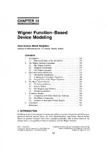
FIG. 3: State space for the one-qubit states ρ = (I + r~σ )/2. The physical states lie within or on the Bloch sphere (BS). The two tetrahedra contain the states positively represented by the Wigner functions W and W , respectively. The state space describable by a non-contextual HVM is a cube with corners (±1, ±1, ±1); also see [44]. It contains the Bloch ball.

The converse of Theorem 2 does not hold: there are quantum states with a non-contextual HVM description for which all considered Wigner functions are negative. This is illustrated in Fig. 3 for the example of a single qubit, where all physically allowed states have an HVM description [1]. The one-qubit states are all of the form ρ = (I + r~σ )/2, and the physical such states are constrained by |r| ≤ 1. The set of states describable in terms of a non-contextual HVM is a cube, |rx |, |ry |, |rz | ≤ 1, containing all physical states. The eight extremal states i of this cube have definite value assignments λi (X), λi (Y ), λi (Z) = ±1 for the observables X, Y , Z. Up to equivalence under translation, there are two one-qubit Wigner functions of type Eq. (6), namely the Wigner function W defined by the phase point operator at the origin A0 = (I + X + Z + Y )/2, and the Wigner function W defined by A0 = HA0 H † = (I+X+Z−Y )/2. The phase space for these Wigner functions is Z2 × Z2 , and W , W thus have four extremal states each. If these extremal states are combined, the extremal states of the non-contextual HVM are recovered. Each Wigner function by itself has only half of the extremal states of the HVM, and the set of positively represented states is thus smaller. Furthermore, there are physical states which are negatively represented by both W and W ; See Fig. 3. Contextuality and negativity of the Wigner functions Eq. (6) are thus not the same. Remark: While there are physical one-qubit quantum states which are negatively represented by both W and W , every state ρ = (I + r~σ )/2, with |rx |, |ry |, |rz | ≤ 1,

Contextuality as a resource

Theorem 3 For any QCSI scheme (γ, M), if the input magic state ρin can be described by a non-contextual HVM, then the quantum state ρt (s≺t ) at time t, conditioned on the prior measurement record s≺t , can be described by a non-contextual HVM, for any t and any s. Before we give the proof of Theorem 3, we need to set up some more notation. We observe that the state space of a general non-contextual HVM is larger than the state space of an HVM deriving from a non-negative Wigner function; See the discussion of a single qubit in Section V C/ Fig. 3. The enlarged state space S = {ν} is finite, yet maximal in the sense that, for every value assignment λ(·) satisfying the consistency condions Eq. (24), there is a corresponding internal state ν ∈ S such that λν (·) ≡ λ(·). We choose to have this state space S acted upon by the group V , dividing S into orbits. Namely, given an element ν ∈ S specified by the value assignment λν : V −→ {±1}, there is another internal state ν +u, defined through the value assignment λν+u (a) = λν (a)(−1)[u,a] , ∀a ∈ V,

(29)

for all u ∈ V . In Eq. (29), we have set λν (a) := λν (Ta ) for notational simplicity. It is easily seen that ν ∈ S ⇔ ν + u ∈ S, for all u ∈ V . The condition to check is the consistency of the value assignment in item (ii) of Def. 3. Eq. (24) is preserved under the change λν (a) 7→ λν (a)(−1)[u,a] , for any u ∈ V . The group action of V on S defined through Eq. (29) labels the elements of S in a fashion convenient for the subsequent discussion. Proof of Theorem 3. The proof of Theorem 3 is by induction. We assume that there exists an HVM with probability distribution qt,s≺t which describes the quantum state ρt (s≺t ), conditioned on the previous measurement record s≺t . We then show that there is an HVM with probability distribution qt+1,s≺t+1 which describes the quantum state ρt+1 (s≺t+1 ). To establish this result, we need the relation between qt+1,s≺t+1 and its precursor qt,s≺t . Denoting the observable measured in the t-th time step of the computation by Tat ∈ O and the corresponding measurement outcome

15 by st ∈ Z2 , the required relation is qt+1,s≺t+1 (ν) =

δ(−1)st ,λν (at ) qt,s≺t (ν) + qt,s≺t (ν + at ) , pt (st |s≺t ) 2 (30a)

pt (st |s≺t ) =

X

δ(−1)st ,λν (at ) qt,s≺t (ν).

(30b)

ν∈S

hTa iqt+1 =

Therein, pt (st |s≺t ) is the HVM prediction for the probability of obtaining the outcome st in the measurement of Tat , given a prior measurement record s≺t . Eq. (30) will be justified a posteriori. Namely, with these assignments, the induction argument works out. With Eq. (23) in Def. 3, the induction assumption is hTa iρt = hTa iqt , ∀a ∈ V. Therein, we have suppressed the dependence on the measurement record, to simplify the notation. We need to show that hTa iρt+1 = hTa iqt+1 , ∀a ∈ V, and that pt (st |s≺t ) = pt (st |s≺t ), with pt (st |s≺t ) the quantum mechanical value for the probability of the outcome st given the prior measurement record s≺t . First, regarding the probability of finding st , X 1 + (−1)st λν (at ) qt,s≺t (ν) 2 ν∈S 1X (−1)st X = qt,s≺t (ν) + qt,s≺t (ν)λν (at ) 2 2

pt (st |s≺t ) =

ν∈S

ν∈S

hIiρt (s≺t ) + (−1)st hTat iρt (s≺t ) = 2   I + (−1)st Tat = Tr ρt (s≺t ) 2

X 1 + (−1)st λν (at )

qt,s≺t (ν)λν (a) 2pt (st |s≺t ) X 1 qt,s≺t (ν)λν (a)+ = 2pt (st |s≺t ) ν∈S (−1)st X + qt,s≺t (ν)λν (a + at ). 2pt (st |s≺t ) ν∈S

ν∈S

Here we have used the relation λν (a + at ) = λν (at )λν (a), which arises as follows. Since Tat ∈ O, Ta ∈ M , and [Tat , Ta ] = 0 by the case assumption, {Tat , Ta } is a jointly measurable set of observables; cf. example (iii) after Def. 2. (The procedure is to measure Tat ∈ O first, and then run the measurement sequence for Ta ∈ M .) Thus, by Property (ii) of Def. 3 for non-contextual HVMs, λν (Tat Ta ) = λν (Tat )λν (Ta ). Finally, with Lemma 1, Tat Ta = Ta+at , which yields the stated relation. Next we use the induction assumption, and obtain 1 (hTa iρt (−1)st + hTa+at iρt ) 2pt (st |s≺t )   1 I + (−1)st Tat = Tr ρt Ta pt (st |s≺t ) 2 i  h st st I+(−1) Tat I+(−1) Tat ρt Ta Tr 2 2 = pt (st |s≺t )

hTa iqt+1 =

= hTa iρt+1 .

= pt (st |s≺t ). We thus reproduce the quantum mechanical expression within the HVM. Above, in transitioning from the second to the third line we have invoked the induction assumption. Second, regarding the expectation values of the Ta on ρt+1 (s≺t+1 ), the HVM prediction is X hTa iqt+1 = qt+1,s≺t+1 (ν)λν (a) ν∈S

=

We now distinguish between the case where Ta , Tat commute and where they don’t. Case (i): [a, at ] = 1. Then, hTa iqt+1 = 0, which is the correct quantum mechanical expression. Case (ii): [a, at ] = 0. Then, the expression for hTa iqt+1 simplifies to

X 1 + (−1)st λν (at )

qt,s≺t (ν)λν (a)+ 4pt (st |s≺t ) X 1+(−1)st λν (at ) qt,s≺t (ν +at )λν (a). + 4pt (st |s≺t ) ν∈S

We thus reproduce the quantum mechanical expression within the HVM. This completes the induction step. The induction starts at time t = 1, where ρ1 = ρin has an HVM description, by assumption of Theorem 3. Thus, by induction, for every time t ≥ 1 and every history s≺t of measurement outcomes, the conditional state ρt (s≺t ) has a description in terms of a non-contextual HVM.  Corollary 1 For any QCSI scheme (γ, M), if the input magic state ρin can be described by a non-contextual HVM, then for the measurement of any sequence of observables {Tat , t = 1..tmax } ⊂ O , the probability distribution p(s) = p(s1 , s2 , .., stmax ) of outcomes is fixed by the HVM for ρin . The Tat may be mutually non-commuting and dependent on previous measurement outcomes. Proof of Corollary 1. By Bayes’ rule, the joint probability of the outcomes s can be written as

ν∈S

Reordering the sum via the substitution ν + at → ν, and using Eq. (29), the second term in the last line equals X 1+(−1)st λν (at ) ν∈S

4pt (st |s≺t )

qt,s≺t (ν)λν (a)(−1)

[a,at ]

.

p(s) =

tY max

pt (st |s≺t ).

t=1

By Theorem 3, the conditional probabilities pt (st |s≺t ) = pt (st |s≺t ) are all correctly obtained from the probability distributions qt,s≺t , cf. Eq. (30b). The distributions

16 qt,s≺t , for t = 2, .., tmax , in turn follow from the distribution q1,s≺1 =∅ (describing ρin at t = 1), by Eq. (30a). Thus, p(s) is fully specified by the probability distribution q1,s≺1 =∅ over the state space S of the HVM.  We now discuss the implications of Theorem 3 with regards to universality of quantum computation. We want to capture in our analysis the case where a QCSI scheme running on n qubits is universal only on a subspace supporting k encoded qubits. (This does of course include the unencoded case, where every logical qubit is represented by one physical qubit.) We use the following notion of computational universality. Definition 4 We say that a QCSI scheme is encoded universal if the following operations can be performed. U1 Encoded inputs. Prepare a set of encoded orthonormal input states E(|xi), x ∈ {0, 1}k up to an arbik n trarily small error , where E : C2 −→ C2 is an isometry of k logical qubits into n physical qubits. k

U2 Encoded gates. For any V ∈ SU (C2 ) and any encoded input state E(|φi) prepare the encoded output state E(V |φi), up to an arbitrarily small error . U3 Encoded outputs. Measure the value of any logical observable E(Xi ), i.e., {E(Xi ), i = 1, .., k} ⊂ O. Requirement U3 means that it is possible to physically measure any logical qubit in the standard basis. We then have the following result. Theorem 4 A QCSI scheme (γ, M) on k ≥ 3 (possibly encoded) qubits satisfying U1 - U3 is universal only if its magic states are contextual. The full proof of Theorem 4 is given in Appendix A. Here we prove Theorem 4 under the simplifying assumption that every encoded qubit can be measured in two complementary bases rather than one basis. That is, U3 is replaced by U30 {E(Xi ), E(Yi ), i = 1, .., k} ⊂ O. While more stringent than U3, the condition U30 is not unreasonable. It grants the measurement device the power to measure two complementary observables for each encoded qubit, and thus to be genuinely quantum. However, the main reason for invoking U30 is that it removes a substantial amount of technical complication from the proof, while preserving its general structure. Proof of Theorem 4 under U 30 . We consider a QCSI where the available initial (magic) states all have an ncHVM description. Now assume that the QCSI scheme is universal for quantum computation. Then, it must be possible to create an encoded Greenberger-Horne-Zeilinger state √ E(|GHZi), with |GHZi = (|000i + |111i)/ 2, on a subset of the qubits from an initial state E(|0i⊗n ). Now consider the expectation value W = hE(X1 X2 X3 )−E(X1 Y2 Y3 )−E(Y1 X2 Y3 )−E(Y1 Y2 X3 )i.

W is a contextuality witness. Since the observables E(Xi ), i = 1, .., 3, are directly measurable by assumption U30 , their product E(X1 X2 X3 ) is inferable, and for any internal state ν of the ncHVM it holds that λν (E(X1 X2 X3 )) =

3 Y

λν (E(Xi )).

i=1

The same holds for the other three measurement contexts (E(X1 ), E(Y2 ), E(Y3 )), (E(Y1 ), E(X2 ), E(Y3 )), and (E(Y1 ), E(Y2 ), E(X3 )). Since for all ncHVM states ν, λν (E(Xi )), λν (E(Xi )) = ±1, for all states ρ describable by an ncHVM it holds that Wρ ≤ 2. However, W|GHZi = 4. The encoded state E(|GHZi) is thus contextual. With Theorem 3, it cannot be prepared by the given QCSI with a non-zero probability of success. Contradiction. The indirect assumption is thus wrong. Hence, if the initial (magic) states are non-contextual, the resulting QCSI scheme is not universal.  Remark: The same conclusion holds when an error  is allowed in the quantum computation, due to the finite gap between of 2 between W|GHZi = 4 and WρHVM ≤ 2. E.

Generalized simulation algorithm

Theorem 5 For any QCSI scheme (γ, M), if (i) the input magic state ρin can be described by a non-contextual HVM with state space S and value assignments λν : V −→ {±1}, for all ν ∈ S, (ii) this HVM can be efficiently sampled from, and (iii) the value assignments λν (a) and the phase convention γ(a) can be efficiently evaluated for all a ∈ VO , then any resulting QCSI can be efficiently classically simulated. Theorem 5 is proved constructively, i.e., by providing a classical simulation algorithm. This algorithm is given in Table II. It is an almost exact copy of the simulation algorithm encountered in Section IV B, and we comment on the resemblance in Section V F. Before we proceed to the proof of Theorem 5, we briefly discuss what sampling from conditional probability distributions means for the above algorithm. For any sample ν drawn in Step 1, while looping through Step 2, a measurement record s is built up. In every iteration t of Step 2, the updated sample νt may be regarded as being drawn from a probability distribution q˜t,s≺t , conditioned on the previous measurement record s≺t . So the above simulation algorithm definitely samples. The question is whether it samples from the correct distributions, i.e., whether q˜t,s≺t = qt,s≺t , for all t = 1, .., tmax and for all s. Proof of Theorem 5. The proof proceeds by demonstrating the correctness and efficiency of the above classical simulation algorithm. Correctness. We first show that for each time t and measurement record s≺t , the above classical simulation

17 Algorithm 2 1. Draw a sample ν ∈ S from the probability distribution q1,s≺1 =∅ describing ρin in the HVM, and set ν1 := ν. 2. For all the measurements of observables Tat ∈ O comprising the circuit, starting with the first, (a) Output the measurement outcome λνt (at ) ∈ {±1} for the observable Tai , using Eq. (29). (b) Flip a fair coin, and update the sample ( νt , if “heads” νt −→ νt+1 = , (31) νt + at , if “tails’ until the measurement sequence is complete. 3. Repeat until sufficient statistics is gathered. TABLE II: Algorithm 2 for the classical simulation of n-qubit QCSI with an ncHVM for the initial state.

algorithm (i) produces the correct quantum-mechanical conditional probability pt (st |s≺t ) of obtaining the outcome st in the measurement of the observable Tat ∈ O, and (ii) samples from the correct conditional probability distribution qt,s≺t of the HVM, which is given by Eq. (30). The proof is by induction. We assume that at time t, the classical simulation algorithm samples from the correct distribution qt,s≺t . Re (i): Denote the conditional probabilities produced by the simulation algorithm as p˜t (st |s≺t ). A state ν ∈ S contributes its probability weight qt,s≺t (ν) to p˜t (0|s≺t ) or p˜t (1|s≺t ) if λν (Tat ) = +1 or λν (Tat ) = −1, respectively. Therefore, X p˜t (st |s≺t ) = δλν (Tat ),(−1)st qt,s≺t (ν) = pt (st |s≺t ). ν∈S

The second equality follows by comparison with Eq. (30b). Furthermore, pt (st |s≺t ) = pt (st |s≺t ) was already demonstrated in the proof of Theorem 3. Thus, p˜t (st |s≺t ) = pt (st |s≺t ), as required. Re (ii): Through the value assignment in step 2(a), an internal state νt ∈ S contributes to q˜t+1,(s≺t ,st =0) , if λνt (at ) = +1, q˜t+1,(s≺t ,st =1) , if λνt (at ) = −1. The update rule for Step 2(a) is thus

F.

Relation between Algorithms 1 and 2

Algorithms 1 and 2 are very similar. They only differ in the sampling source they have access to. By Theorem 2, the sampling source for Algorithm 2, based on noncontextual HVMs, is at least as powerful as the sampling source for Algorithm 1, based on non-negative Wigner functions. By the 1-qubit example of Section V C, the former source is indeed more powerful. In the following, we investigate the relation between the two sampling sources in greater detail. The result is that if the initial quantum state ρin can be described by a non-contextual HVM, then it can be represented by an ensemble Eρin = {(pi , ρi )} , such that there are Wigner functions W γi for which (i) Wργii ≥ 0, ∀i, and (ii) the measurement of observables from the set O preserves positivity of the W γi , ∀i. Therefore, Algorithm 2 can be simulated by a master algorithm that merely draws samples ν ∈ S from the non-contextual HVM, and then employs Algorithm 1 as a subroutine for dealing with the samples. This interpretation of Algorithm 2 is developed below. The state space S of the HVM can be partitioned into orbits [ν] of V , [ν] = {ν + u, u ∈ V } ∈ S/V.

st δλ (a ),(−1)st 0 qt,s≺t (τ ) −→ qt+1,s (τ ) = qt,s≺t (τ ) τ t , ≺t+1 pt (st |s≺t ) for all τ ∈ S, and pt (st |s≺t ) appears for normalization. In step 2(b), with Eq. (31), the update rule is 0 0 qt+1,s −→ q˜t+1,s≺t+1 = qt+1,s ∗ ≺t+1 ≺t+1

where “∗” stands for convolution. Using Eq. (29), the resulting expression for q˜t+1,s≺t+1 (ν) matches the expression in Eq. (30a), i.e., q˜t+1,s≺t+1 (ν) = qt+1,s≺t+1 (ν), as required. This completes the induction step. The induction assumption is satisfied for t = 1, by the first assumption of Theorem 5. Thus, by induction, the above algorithm samples from the correct conditional outcome probabilities p(st |s≺t ) for measurement outcomes st and from the correct HVM distributions qt,s≺t describing ρt (s≺t ), for all times t and all outcome histories s. Efficiency. The classical preprocessing of removing the unitaries g ∈ G from the circuit is efficient if the function γ : V −→ Z4 can be efficiently computed, which holds by assumption. See the proof of Theorem 1. Regarding the simulation algorithm itself, the critical step is 2(a), the evaluation of the function λν on some a ∈ V . Again, the efficiency of this function evaluation is guaranteed by the assumption of the theorem. 

δ0 + δat , 2

Then there exists a special orbit [0] ∈ S/V defined by the property that there is a τ[0] ∈ [0] for which the value assignment is constant, λτ[0] (·) ≡ 1. With Eq. (29) it then follows that λτ[0] +u (a) = (−1)[u,a] , ∀a ∈ V. Comparing with Eq. (20), we find that the above value assignment λτ[0] +u (a) agrees with the value assignment

18 made by a positive Wigner function Eq. (6) considered as an HVM, if we identify, for all u ∈ V ,

HVM sampler

(τ[0] + u) ∈ [0] ←→ u ∈ V. This motivates the definition of a quantum state ρ[0] associated with the orbit [0], via Wρ[0] (u) :=

q(τ[0] + u) , ∀u ∈ V, p[0]

p1 γ

(32)

p2

p3

γ

Wρ11

Wρ22

Wρ33

sampler

sampler

sampler

γ

P

where p[0] = u∈V q(τ[0] +u) to ensure proper normalization. The state ρ[0] (u) is not required to be a valid quantum state, i.e., to be positive semi-definite. The only requirement is a non-negative Wigner function, which is satisfied by definition. The fact that classical sampling algorithms can handle states which have a positive Wigner function but are not proper quantum states is familiar from the qudit case [10]. In analogy with Eq. (32), we will now define states ρ[ν] for all orbits [ν] ∈ S/V . The state ρ[0] and its cousins will then be used in the interpretation of Algorithm 2. For any [ν] ∈ S/V , pick a τ[ν] ∈ [ν] and define γ

Ta [ν] := λ−1 τ[ν] (a)Ta , ∀a ∈ V,

(33)

where on the r.h.s. Ta = Taγ , as defined in Eq. (5). Denoting λτ[ν] (a) = (−1)s[ν] (a) , for all a ∈ V , we thus have the relation γ[ν] ≡ γ + 2s[ν]

mod 4.

(34)

γ γ
From the above definition of Ta [ν] , λτ[ν] Ta [ν] = 1, for all a ∈ V . We can thus reproduce for any orbit [ν] the previous argument for [0]. First, with Eq. (29), γ
λτ[ν] +u Ta [ν] = (−1)[a,u] , ∀a, u ∈ V. (35)

Again by comparison with Eq. (20), the value assignments by the HVM and by the Wigner function W γ[ν] match if we identify, for all u ∈ V , (τ[ν] + u) ∈ [ν] ←→ u ∈ V.

(36)

A state ρ[ν] associated with any orbit [ν] ∈ S/V can now be defined, via γ

[ν] Wρ[ν] (u) :=

q(τ[ν] + u) , ∀u ∈ V. p[ν]

(37)

P Therein, p[ν] = u∈V q(τ[ν] + u). As before with ρ[0] (u), the state ρ[ν] (u) is not required to be positive semidefinite. Remark: For each [ν] ∈ S/V , the choice of the representative τ[ν] is arbitrary. Different choices lead to different γ[ν] , which are, however, related in a simple way. Namely, the corresponding Wigner functions differ only by translation. By contrast, the Wigner functions W γ[ν] and W γ[ν 0 ] , for any [ν 0 ] 6= [ν], are not equivalent under translation.

FIG. 4: Relation between Algorithms 1 and 2. Sampling from the probability distribution underlying a non-contextual HVM may be viewed as a two-stage process. Stage 1: Sampling from a probability distribution {pi } over Wigner functions, Stage 2: Sampling from the phase space w.r.t. to the Wigner function chosen in the first stage.

With the above, we can now re-interpret the sampling from the HVM as the following two-stage process. In the first stage, equivalence classes [ν] ∈ S/V are sampled from, according to the probabilities {p[ν] }. In the second stage, given a particular class [ν], the phase space V is sampled from, according to the conditional probability distribution q|[ν] /p[ν] . The conditional probability distributions q|[ν] /p[ν] over V are regarded as Wigner funcγ[ν] of states ρ[ν] associated with the orbits [ν], tions Wρ[ν] cf. Eq. (37). See Fig. 4 for illustration. Algorithm 2 can thus be simulated by a master algorithm calling Algorithm 1 as a subroutine, as follows. Step 1: A sample ν ∈ S is drawn. This sample is converted into the into the pair ([ν] ∈ S, u ∈ V ), such that ν = τ[ν] + u. Step 2: Algorithm 1 is called, with the sample u1 := u being handed over. The orbit [ν] has no influence on how Algorithm 1 runs, but needs to be taken into account when the simulated measurement outcomes are returned. Namely, Algorithm γ 1 returns the values for Tat[ν] , not for the Tat with the standard phase convention γ. A conversion of those values is thus necessary, which proceeds by Eq. (33). There is one more item to check: To employ sampling from Wigner functions W γ[ν] as a subroutine, the measurement of observables which leave positive Wigner functions W positive must also leave all Wigner functions W γ[ν] positive. Denote by O[ν] the non-extendable set of directly measurable observables w.r.t. the phase convention γ[ν] (i.e., the set of Pauli observables whose measurement preserves non-negativity of the Wigner function W γ[ν] ). Then, we have the following result. Lemma 9 For all [ν] ∈ S/V , it holds that O[ν] = O. In addition, we note that the states ρ[ν] , defined in Eq. (37) have the following relation to the input state ρin of the computation. Lemma 10 For any QCSI scheme (γ, M), if the input state ρin has a non-contextual HVM description, then

19 the states ρ[ν] provide an ensemble representation Eρin =  (p[ν] , ρ[ν] ), [ν] ∈ S/V of ρin , i.e., X

ρin =

p[ν] ρ[ν] .

VI. A QUBIT SCHEME OF QCSI WITH MATCHING WIGNER FUNCTION A.

(38)

Definition of the Wigner function

[ν]∈S/V

Multiple Wigner functions have previously been discussed in the context of QCSI [11]. Therein, a quantum state is considered classical if all its Wigner functions are positive. Our viewpoint is the opposite. For a state to be considered classical, not even a single one of its Wigner functions has to be positive. Proof of Lemma 9. By Eq. (8), for any phase convention γ it holds that β(a, b) = γ(a) + γ(b) − γ(a + b) + 2aX bZ

In this section we focus on the properties of a single Wigner function. We make the choice γ0 (a) = aZ · aX mod 4,

(39)

which has the important and rare consequence that the corresponding Wigner function factorizes, Wρ⊗σ = Wρ · Wσ for all states ρ, σ. In fact, the factorization property already holds on the level of the Heisenberg-Weyl operators Eq. (5),

mod 4.

Ta ⊗ Tb = Ta+b .

(40)

Then, by Eq. (34), the function β based on a specific γ and the functions β[ν] based on the corresponding γ[ν] are related via B.

The set O of directly measurable observables


β[ν] (a, b) = β(a, b) + 2 s[ν] (a) + s[ν] (b) − s[ν] (a + b) , where the addition is again mod 4. Now assume that Ta ∈ O and that [a, b] = 0. Then, {Ta , Tb } is a jointly measurable set of observables, and thus, by Property (ii) of Def. 3, s[ν] (a)+s[ν] (b)−s[ν] (a+b) mod 2 = 0. Hence, β[ν] (a, b) = β(a, b), ∀ [ν] ∈ S/V, for all above pairs a ∈ VO , b ∈ V . Thus, by Lemma 1, the measurement of Ta preserves positivity of the Wigner function W γ if and only if it preserves positivity of the Wigner function W γ[ν] , for any [ν] ∈ S/V .  Proof of Lemma 10. Since the Ta , a ∈ V , form a basis of Hermitian operators on n qubits, it suffices to show that hTa iρin = hTa iP[ν] p[ν] ρ[ν] , for all a ∈ V . hTa iP[ν] p[ν] ρ[ν] =

X

p[ν] hTa iρ[ν]

= =

X

γ

p[ν] λτ[ν] (a)hTa [ν] iρ[ν]

[ν]

p[ν] λτ[ν] (a)2n

=

λτ[ν] (a)

X

X

γ[ν] γ[ν]

Ta

(u)

[a,u]

q(τ[ν] + u)(−1)

u∈V

[ν]

=

γ

[ν] Wρ[ν] (u)W

u∈V

[ν]

X

X

γ

q(ν)λτ[ν] (a)λν Ta [ν]




ν∈S

=

X

O = {±Xi , ±Yi , ±Zi |, i = 1, .., n}. This means first of all that the corresponding Wigner function W γ0 has a corresponding QCSI scheme, and, perhaps surprisingly, spatial locality plays a role in it. Below, we first prove Lemma 11, and then flesh out the QCSI scheme corresponding to W γ0 . Proof of Lemma 11. We first show that the set O = {Xi , Yi , Zi |, i = 1, .., n} satisfies the defining conditions Eqs. (10), (14). Consider two commuting Pauli observables Tb , Tc such that Tb is local to qubit k, and Tc is written as Tc = Tc0 +c00 = Tc0 ⊗ Tc00 , where Tc0 acts nontrivially only on qubit k, and Tc00 acts nontrivially only on the complement of qubit k. Then, Tb Tc = = = =

[ν]

X

Lemma 11 For γ0 (a) = aZ · aX mod 4, the set O of directly measurable observables is

q(ν)λν (Ta )

ν∈S

= hTa iρin , as required. We used Eq. (33) in line 2 above, Eq. (37) in line 4, Eq. (35) in line 5, and Eq. (33) in line 6. 

Tb Tc0 ⊗ Tc00 0 i−β(b,c ) Tb+c0 ⊗ Tc00 0 i−β(b,c ) T(b+c0 )+c00 0 i−β(b,c ) Tb+c .

Therein, in lines 1 and 3 we used the property Eq. (40). Since Tb and Tc are commuting, β(b, c0 ) ∈ {0, 2}. Since Tb is local, by going through all the cases of local Pauli operators we find that β(b, c0 ) ∈ {0, ±1}. Thus, β(b, c0 ) = 0 is the only choice that satisfies both constraints. Therefore, Tb+c = Tb Tc ,

(41)

whenever [Tb , Tc ] = 0, and Tb is local. Condition (10) is thus satisfied. Next, since every multi-local Pauli operator can be written as a tensor product of local Pauli operators, and

20 the local Pauli operators in such an expansion trivially commute, it follows that VM = V , as required by condition (14). We have thus shown that {Xi , Yi , Zi |, i = 1, .., n} is a possible set O. It remains to prove that the above O is maximal, i.e., that O cannot contain any additional observable without violating the condition Eq. (10). For n = 1 this is clear, and we only need to discuss the case of n ≥ 2. To this end, consider the two-local Pauli operators, beginning with Y ⊗ Y .

X2

X1 Z2

β=0

XZ

XX β=2

Z1

ZX

ZZ

(a)

(b) Z

Z

Z

Z

Z

Z

Z

Z

Z

Z

Z

Z

Z

Z

X

X

X

X

X

X

X

X

X

X

Z

X

X

X

Z

Z

Z

Z

Z

Z

Z

Z

Z

X

X/Y

X

Z

Z

Z

Z

Z

Z

Z

Z

Z

Z

Z

Z

Z

Z

Z

Z

FIG. 5: QCSI with modified cluster state of Eqs. (42a), (42b) as magic state, which is subjected to measurements of local Pauli operators Xi , Yj , Zk , for all i, j 6= i, k 6= i, j ∈ V. The role of the Z-measurements is to cut out of the plane a web corresponding to some layout of a quantum circuit, and the X-measurements drive the MBQC-simulation of this circuit [45]. The qubit in R is displayed in red. By “re-routing” a wire piece, one may choose between implementing and not implementing a non-Clifford gate. (a) Identity operation on the logical state space, (b) Logical gate eiπ/4 Z .

YY C.

Y ⊗ Y is part of a context with β = 2 6= 0 mod 4. Therefore, with Lemma 1, Y ⊗ Y 6∈ O. Now, conjugate the observables in the above diagram under a local Clifford unitary, and readjust the signs such that only observables Ta appear. In this way, any twolocal Pauli observable can appear in the bottom left corner of the diagram. We observe that the four observables in the top left corner of the diagram will remain local under such a transformation. As we have shown, all local Pauli operators Tb satisfy Eq. (41) for all commuting Tc . Hence, (i) The four βs involving local observables remain β = 0. (ii) The six β appearing in the square must sum to 2 mod 4, as per Mermin’s argument. Combining these two facts, we find that the two β involving the observable in the bottom right corner of the diagram cannot simultaneously be zero. Hence this observable cannot be in O. Thus, no two-local Pauli observable is in O. Next, consider a Pauli observable Tb with a support of size greater than 2. Be J a set of two sites in the support of Tb , J = {j, k} ⊂ supp(Tb ), and denote by Tb0 the restriction of Tb to J, and by Tb00 the restriction of Tb to the complement of J. Then, with Eq. (40), Tb = Tb0 +b00 = Tb0 ⊗ Tb00 . Now consider a second Pauli operator Tc that commutes with Tb and has support on J only. Then, using the property Eq. (40), Tb Tc = = = =

Tb00 ⊗ Tb0 Tc 0 iβ(b ,c) Tb00 ⊗ Tb0 +c 0 iβ(b ,c) Tb00 +(b0 +c) 0 iβ(b ,c) Tb+c .

By the previous argument for two-local operators, for any Tb with support on two or more qubits, a commuting twolocal Pauli operator Tc can be found such that β(b0 , c) = 2. Then, with Lemma 1, ±Tb 6∈ O.  From Eq. (4) it follows that the set Ω of free states are tensor products of one-qubit stabilizer states. The group of free unitary gates therefore is the local Clifford gates.

Magic states and universality

From the perspective of computational universality of QCSI, all we don’t know yet is what the magic states are. Since all state preparations and measurements are local in the present situation, any entanglement needed in the computation must be brought in by the magic state. That is, there is only one big entangled magic state. Factors of tensor product states cannot be coupled by the free operations. In fact, one possibility is to use as magic state a slightly modified cluster state. We consider a set of qubits located on the vertices of a square lattice graph. We denote the set of its sites by V and its adjacency matrix by Γ. We single out a subset R ⊂ V of sites which are sufficiently √ . With those sparse. Denote by A the observable X+Y 2 definitions the resource state |Ψi is the unique joint eigenstate with eigenvalue 1 of the stabilizer operators O KaX := Xa Zb Γab , if a ∈ V\R, (42a) b∈V

KaA

:= Aa

O

Zb Γab , if a ∈ R.

(42b)

b∈V

That this leads to universal quantum computation is easily shown by standard arguments pertaining to measurement-based quantum computation (MBQC). See Fig. 5 for illustration. While being a valid scheme of QCSI, this is also MBQC. The distinction between MBQC and QCSI is thus blurred. By various equivalence transformations, we can make the above computational scheme look more like the known QCSI schemes, or more like standard MBQC. Equivalent scheme 1. In all QCSI schemes worked out to date [11], [10], [7], [8], the magic states are local to single or at most 2 particles. Although this is by no means necessary, we are used to those states being injected into the computation one by one. If desired, we may convert the above computational scheme into such a form,

21 by conjugating it—the resource state, the measurable observables in O, and the Wigner function W 0 —under the unitary transformation Y Γ (43) UIsing = (Λ(Z)i,j ) ij . i,j∈V

In this way, we arrive at the following equivalent computational scheme. The resource state |Ψi is converted into a tensor product state of individual qubits being in the state |+ii , defined by X|+i = |+i, for i ∈ V\R, and |Aij , defined by A|Ai = |Ai, for j ∈ R. The new magic states are thus the local states |Aij . The new set O1 of directly measure observables N is O1 = {KaX , KaY , Za , a = 1, .., n}, where KaY = Ya b∈V Zb Γab . Equivalent scheme 2. We note in Eq. (42b) that stabilizer operators K A of the magic state |Ψi are not exactly stabilizer operators of cluster states. Therefore, we may apply the equivalence transformation O Uloc = e−iπ/4 Zj , j∈R

and obtain as the new magic state the standard cluster state. The new measurable observables are O2 = {Xi , Yi , Aj , A0j , Zk | a ∈ V\R, j ∈ R, k = 1..n}, √ where A0 = (X − Y )/ 2. We note that the measurable observables which are not Zs are of the form Oi = cos φi Xi ± sin φi Yi , as standard in MBQC [45]. A minor deviation from the standard remains. Namely, for each site i, only a single setting out of two is available for the measurement angle, either φi = 0 or φi = π/4. In standard MBQC, any angle φi ∈ [0, π/2] may be chosen. However, the present restriction does not affect computational universality.

VII.

CONCLUSION

In this paper, we have constructed a tomographically and informationally complete QCSI scheme for qubits in which contextality of the magic states is necessary for quantum computational universality. This case had remained open after the previously described schemes for qudits [7] and rebits [8]. More generally, we have shown that for all QCSI schemes on qubits satisfying the postulate (P3), for k ≥ 3 qubits, contextuality is necessary for quantum computational universality. We also investigated the role of Wigner functions for the qubit case. The purpose of the Wigner function W γ is to explain the near-classicality of the free sector of QCSI, i.e. the operations in QCSI which are not considered resources. We found the following features of interest: (i) In contrast to the qudit and the rebit case described in the literature, for general QCSI schemes on qubits, the

free unitary gates may introduce negativity into Wigner functions without compromising efficient classical simulability. The violation of positivity can be very large as measured by the sum negativity [42]. (ii) Any choice Eq. (5) of the phase convention γ for the Wigner function W γ uniquely determines the free sector of a corresponding QCSI scheme. To summarize, in this work we have used classical simulation of quantum computation as a tool to identify quantum resources required for a speed-up. More generally, determining the cost of simulating universal quantum computing classically is fascinating open question; See e.g. [46], [47]. Acknowledgments. RR thanks Terry Rudolph and the Horodecki family for discussion. This work has been funded by NSERC (ND, CO and RR), SIQS (JBV), AQuS (JBV), Cifar (ND and RR), and IARPA (RR). RR is Fellow of the Cifar Quantum Information Program.

Appendix A: Proof of Theorem 4

Before we give the proof, we need to set up some additional notation. Namely, we extend the value assignments λν . As per Eq. (31) in the simulation Algorithm 2 of Section V E, the update of the internal state ν in the measurement of an observable Tat invokes a random bit ct , νt −→ νt+1 = νt + ct at . Assume, the measurement sequence representing a given quantum algorithm has a maximum length tmax . Since these values {ct , t = 1, .., tmax } are random and uncorrelated with everything, it does not matter whether they are determined at runtime or before the computation, and we may include those values in the ncHVM value assignments λν . That is, we extend the internal states ν ∈ S to ν ∗ = (ν, c1 , c2 , . . . , ctmax ). Correspondingly, the set of internal states becomes S ∗ := max S × Z×t . 2 A consequence of this definition is that the function λν can now assign a value to a potentially larger set of observables than the inferable ones. Namely, consider a unitary U which can be implemented using free gates, free measurements and ancilla states that can be described by an ncHVM, and an inferable observable O ∈ M . Then, the observable U † OU can also be measured, namely by first implementing U and then measuring O. However, it is not a priori clear that U † OU ∈ M . Yet, by the general simulation Algorithm 2, given the initial internal state ν ∗ , a value λν ∗ (U † OU ) can be assigned to the observable U † OU . An important point to note is that the value assignments involving quantum circuits are in general context dependent. That is, they depend on how the unitary U is implemented as a circuit, and which acilla states are being consumed in the process. Further, for two given

22 observables O ∈ M , O0 , related via O0 = U † OU , the unitary U is not unique, and λν ∗ (U † OU ) may again depend on the choice made. It is this potential contextuality of value assignments involving circuits that complicates the proof of Theorem 4. Let’s illustrate this property in an example. Suppose there is a QCSI setting where all observables Xi can be directly measured but Y3 cannot. Further, assume that the unitary S3 , with the property Y3 = S3† X3 S3 , can be implemented using only free operations and ancillas that have an ncHVM description. The circuit for measuring Y3 in this example is to first implement S3 and then measure X3 . Now the task is to measure Y3 after first measuring either X1 or X2 . Are the corresponding values λν ∗ (Y3 ) assigned by the internal state ν ∗ via the simulation Algorithm 2 the same in those two situations? This is in general not the case. Suppose that ν ∗ is such that c1 = 1. Then, if X1 was measured first, the HVM state after the first measurement is ν + aX1 . Analogously, if X2 was measured first, the HVM state after the first measurement is ν + aX2 . With the second measurement in the sequence begins the implementation of the measurement of Y3 . By construction, the measurement strategy does not depend on the outcome of the first measurement. Therefore, the second measured observable is the same Ta2 in both cases. However, the value assigned to this observable by the internal state ν ∗ through Eq. (29) differs if [a2 , aX1 ] 6= [a2 , aX2 ]. In this situation, the HVM prediction for the outcome obtained in the second measurement depends on which observable was measured first. Since the choice of observable in the third measurement may depend on the outcome of the second measurement, the two measurement sequences may now run down completely different tracks, and there is no guarantee whatsoever that the value assigned to Y3 will be the same. Hence, the value assignments involving circuits are potentially contextual. Proof of Theorem 4. The outline of the proof is as follows. Suppose the statement is wrong, i.e., it is possible that the initial magic state has a description of an ncHVM and simultaneously gives rise to universal quantum computation. Then, by assumptions U1 and U2, universality implies that an encoded GHZ-state can be prepared. Further, by U2 and U3 it is possible to randomly measure in one of the four contexts E(X1 , X2 , X3 ), E(X1 , Y2 , Y3 ), E(Y1 , X2 , Y3 ), E(Y1 , Y2 , X3 ). In each such measurement, the three outcomes are multiplied and it is verified whether the product matches the corresponding stabilizer eigenvalue of the GHZ state. We will show below that if the initial (magic) state has an ncHVM description, then the simulation Algorithm 2 will fail to reproduce the quantum prediction for the stabilizer eigenvalues of the GHZ-state with a probability ≥ 1/8. However, Algorithm 2 has been proven to be correct (See Theorem 5), and therefore computational universality and availability of an ncHVM description for the initial state cannot simultaneously apply.

We now describe the measurement procedures for the four measurement contexts. Case (i): E(X1 , X2 , X3 ). The three observables E(X1 ), E(X2 ), E(X3 ) are jointly measured, which is guaranteed to be possible by U3. Case (ii): the three remaining contexts E(Xi , Yj , Yk ), i 6= j 6= k ∈ {1, 2, 3}. For each of the three measurement contexts, we apply the following procedure: 1. Measure the observable E(Xi ). 2. Implement the measurement sequence corresponding to the execution of the encoded gate E(S1 ⊗ S2 ⊗ S3 ), giving rise to a free unitary g ∈ G which is propagated out of the circuit; See Fig. 2. 3. Measure the observables g † E(Xi )g, for i = 1, .., 3. The outcomes for E(Y1 ), E(Y2 ) and E(Y3 ) are thereby obtained. Among them, the value for E(Yi ) is discarded. Step 1 of this procedure is possible by U3, Step 2 is possible by U2. Regarding Step 3, the unitary g is in general dependent on them measurement outcomes obtained in implementing the circuit for E(S1 ⊗ S2 ⊗ S3 ), but in all cases g is free (g ∈ G). Thus, the observables g † E(Xi )g are in O and can be directly measured. From the perspective of the hidden variable model, for any internal state ν ∗ ∈ S ∗ , the values λν ∗ (E(Xi )), λν ∗ (E(Yi )), i = 1, .., 3 are assigned to the corresponding observables via the simulation Algorithm 2 applied to the above measurement procedure. We now show that these value assignments are non-contextual if c1 = 0. (i) E(Xi ). Since the E(Xi ) are measured first in every context they appear in, λν ∗ (E(Xi )) = λν (E(Xi )). They are thus context independent. (ii) E(Yi ). We show this by the example of E(Y1 ), the other two cases are analogous. E(Y1 ) appears in two measurement contexts, namely E(Y1 , X2 , Y3 ) and E(Y1 , Y2 , X3 ). The corresponding measurement procedure differ only in one respect. In the former context E(X2 ) is measured in the first step, and in the latter context E(X3 ) is measured in the fist step. Now, by the assumption of c1 = 0, the internal state ν remains unchanged under this first measurement in both cases, and in particular remains the same for both cases. After the first step, the procedures are thus identical, and the same value λν ∗ (E(Y1 )) is assigned by the HVM in either context. Thus, if c1 = 0, all values λν ∗ (E(Xi )), λν ∗ (E(Yi )), i = 1, .., 3 assigned by the HVM are thus non-contextual, as claimed. By Mermin’s argument, such non-contextual value assignments fail to reproduce the respective stabilizer eigenvalue of the encoded GHZ-state in at least one of the contexts. Thus, if the measurement contexts are randomly chosen, if c1 = 0 then the HVM fails to match the quantum prediction with a probability of ≥ 1/4. Further, for any internal state ν ∈ S, the conditional probability for c1 = 0 in ν ∗ given ν equals 1/2 (recall that c1 is the result of an unbiassed coin flip). Therefore,

23 measurement record with a probability ≥ 1/8.

the HVM fails to match the quantum prediction with a probability ≥ 1/8. Finally, universality only requires the preparation of an encoded GHZ-state E(|GHZi) up to an arbitrarily small error  > 0, and likewise only the approximate realization of the gates E(Si ), up to the same error . When taking such errors into account, the HVM prediction remains unchanged. If the initial state can be described by a non-contextual HVM, the measurement record will fail to reproduce the quantum mechanical prediction of the

The quantum prediction does now differ from the ideal scenario. With a slightly erroneous encoded GHZ-state E(|GHZi) and slightly erroneous gates E(Si ), the measurement record will differ from the measurement record for the ideal circuit with a probability p(). However, p() can be made arbitrarily small by decreasing . Thus, even in the presence of a small error , the quantum prediction can be distinguished from the HVM prediction. 

[1] J.S. Bell, On the Problem of Hidden Variables in Quantum Mechanics, Rev. Mod. Phys. 38, 447 (1966). [2] S. Kochen and E.P. Specker, The Problem of Hidden Variables in Quantum Mechanics, J. Math. Mech. 17, 59 (1967). [3] N. D. Mermin, Hidden Variables and the Two Theorems of John Bell, Rev. Mod. Phys. 65, 803 (1993). [4] Samson Abramsky, Adam Brandenburger, The sheaftheoretic structure of non-locality and contextuality, New J. Phys. 13, 113036 (2011). [5] Adan Cabello, Simone Severini, Andreas Winter, GraphTheoretic Approach to Quantum Correlations, Phys. Rev. Lett. 112, 040401 (2014). [6] A. Ac´ın, T. Fritz, A. Leverrier, A. Bel´en Sainz, A Combinatorial Approach to Nonlocality and Contextuality, arXiv:1212.4084. [7] M. Howard et al., Nature (London) 510, 351 (2014). [8] N. Delfosse, P. Allard-Guerin, J. Bian and R. Raussendorf, Wigner Function Negativity and Contextuality in Quantum Computation on Rebits, Phys. Rev. X 5, 021003 (2015). [9] S. Bravyi and A. Kitaev, Universal Quantum Computation with Ideal Clifford Gates and Noisy Ancillas, Phys. Rev. A 71, 022316 (2005). [10] V. Veitch, C. Ferrie, D. Gross, and J. Emerson, Negative Quasi-probability as a Resource for Quantum Computation, New J. Phys. 14, 113011 (2012). [11] E. F. Galvao, Discrete Wigner Functions and Quantum Computational Speedup, Phys. Rev. A 71, 042302 (2005). [12] Cecilia Cormick, Ernesto F. Galvao, Daniel Gottesman, Juan Pablo Paz, Arthur O. Pittenger, Classicality in discrete Wigner functions, Phys. Rev. A 73, 012301 (2006). [13] E. Wigner, On the Quantum Correction For Thermodynamic Equilibrium, Phys. Rev. 40, 749 (1932). [14] K.S. Gibbons, M.J. Hoffman, and W.K. Wootters, Discrete Phase Space Based on Finite Fields, Phys. Rev. A 70, 062101 (2004). [15] D. Gross, Computational power of quantum many-body states and some results on discrete phase spaces, PhD Thesis, Imperial College London, 2005. [16] A. Mari, J. Eisert, Positive Wigner functions render classical simulation of quantum computation efficient, Phys. Rev. Lett. 109, 230503 (2012). [17] R.L. Hudson, When is the Wigner quasi-probability density non-negative?, Rep. Math. Phys. 6, 249 (1974). [18] Robert W. Spekkens, Negativity and contextuality are equivalent notions of nonclassicality, Phys. Rev. Lett. 101, 020401 (2008). [19] Huangjun Zhu, Permutation symmetry determines the

discrete Wigner function, arXiv:1504.03773. [20] Huangjun Zhu, Multiqubit Clifford groups are unitary 3designs, arXiv:1510.02619. [21] N. D. Mermin, Extreme quantum entanglement in a superposition of macroscopically distinct states, Phys. Rev. Lett. 65, 1838 (1990) . [22] V. Scarani, A. Acin, E. Schenck, and M. Aspelmeyer, Nonlocality of cluster states of qubits, Phys. Rev. A 71, 042325 (2005). [23] O. G¨ uhne, G. Toth, P. Hyllus, and H. J. Briegel, Bell inequalities for graph states, Phys. Rev. Lett. 95, 120405 (2005). [24] Juan Bermejo-Vega, Nicolas Delfosse, Cihan Okay, Dan E. Browne, Robert Raussendorf, Contextuality as a resource for qubit quantum computation, in preparation. [25] D. Gottesman, Stabilizer Codes and Quantum Error Correction, Ph.D. thesis, California Institute of Technology, 1997. [26] Mark Howard, Eoin Brennan, Jiri Vala, Quantum Contextuality with Stabilizer States, Entropy 15, 2340 (2013). [27] Y. Han, L. Hemaspaandra and T. Thierauf, Threshold computation and cryptographic security, SIAM J. on Computing 26, 59 (1997). [28] S. Aaronson, Quantum computing, post-selection and probabilistic polynomial time, Proc. R. Soc. A 461, 3473 (2005). [29] S. Aaronson and A. Arkhipov, Proc. of ACM STOC, 333342, (2011). [30] M. J. Bremner, R. Jozsa, and D. J. Shepherd, Classical simulation of commuting quantum computations implies collapse of the polynomial hierarchy, Proc. R. Soc. A 467, 459 (2011). [31] Tomoyuki Morimae, Keisuke Fujii, Joseph F. Fitzsimons, On the hardness of classically simulating the one clean qubit model, Phys. Rev. Lett. 112, 130502 (2014). [32] Matty J. Hoban et al., Measurement-based classical computation, Phys. Rev. Lett. 112, 140505 (2014). [33] N.D.Mermin, Simple Unified Form for No-HiddenVariables Theorems, Phys.Rev.Lett. 65, 3373 (1990). [34] A.Peres, Incompatible results of quantum measurements, Phys. Lett. A 151, 107-8 (1990). [35] A. R. Calderbank, Peter W. Shor, Good Quantum ErrorCorrecting Codes Exist, Phys. Rev. A 54, 1098 (1996). [36] Andrew Steane, Multiple Particle Interference and Quantum Error Correction, Proc.Roy.Soc.Lond. A 452, 2551 (1996). [37] D. W. Kribs, R. Laflamme, D. Poulin, and M. Lesosky, Operator quantum error correction, QIC 6, 382 (2006). [38] D. Poulin, Stabilizer formalism for operator quantum er-

24 ror correction, Phys. Rev. Lett. 95, 230504 (2005). [39] D. Bacon, Operator quantum error-correcting subsystems for self-correcting quantum memories, Phys. Rev. A 73, 012340 (2006). [40] P. W. Shor, Scheme for reducing decoherence in quantum computer memory, Phys. Rev. A 52, 2493 (1995). [41] H. Bombin, Topological Subsystem Codes, Rev. A 81, 032301 (2010). [42] Victor Veitch, Seyed Ali Hamed Mousavian, Daniel Gottesman, Joseph Emerson, The Resource Theory of Stabilizer Computation, New J. Phys. 16, 013009 (2014). [43] Hakop Pashayan, Joel J. Wallman, Stephen D. Bartlett, Estimating outcome probabilities of quantum circuits us-

[44]

[45] [46]

[47]

ing quasiprobabilities, Phys. Rev. Lett. 115, 070501 (2015). Joel J. Wallman, Stephen D. Bartlett, Nonnegative subtheories and quasiprobability representations of qubits, Phys. Rev. A 85, 062121 (2012). R. Raussendorf and H.J. Briegel, A one-way quantum computer, Phys. Rev. Lett 86, 5188 (2001). M. Van den Nest, W. D¨ ur, G. Vidal, H. J. Briegel, Classical simulation versus universality in measurement based quantum computation, Phys. Rev. A 75, 012337 (2007). Sergey Bravyi, Graeme Smith, John Smolin, Trading classical and quantum computational resources, arXiv:1506.01396.