Continuity and differentiability of set-valued maps revisited in the light of tame geometry A RIS DANIILIDIS & C. H. J EFFREY PANG Abstract Continuity of set-valued maps is hereby revisited: after recalling some basic concepts of variational analysis and a short description of the State-of-the-Art, we obtain as by-product two Sard type results concerning local minima of scalar and vector valued functions. Our main result though, is inscribed in the framework of tame geometry, stating that a closed-valued semialgebraic set-valued map that does not necessarily have closed graph is almost everywhere continuous (in both topological and measure-theoretic sense), strictly continuous and strictly differentiable (as set-valued map). The result –depending on stratification techniques– holds true in a more general setting of o-minimal (or tame) set-valued maps. Some applications are briefly discussed at the end. Key words Set-valued map, (strict, outer, inner) continuity, Aubin property, set-valued differentiability, semialgebraic, piecewise polyhedral, tame optimization. AMS subject classification Primary 49J53 ; Secondary 14P10, 57N80, 54C60, 58C07.
Contents 1 Introduction
1
2 Basic notions in set-valued analysis 2.1 Continuity concepts for set-valued maps . . . . . . . . . . . . . . . . . . . . . . . . . . 2.2 Normal cones, coderivatives and the Aubin property . . . . . . . . . . . . . . . . . . . . 2.3 Differentiability for set-valued maps . . . . . . . . . . . . . . . . . . . . . . . . . . . .
3 3 4 6
3 Preliminary results in Variational Analysis 3.1 Sard result for local (Pareto) minima . . . . . . . . . . . . . . . . . . . . . . . . . . . . 3.2 Extending the regularity criterion and a critical value result . . . . . . . . . . . . . . . . 3.3 Linking sets . . . . . . . . . . . . . . . . . . . . . . . . . . . . . . . . . . . . . . . . .
7 7 9 10
4 Generic continuity of tame set-valued maps 4.1 Semialgebraic and definable mappings . . . . . . . . . . . . . . . . . . . . . . . . . . . 4.2 Some technical results . . . . . . . . . . . . . . . . . . . . . . . . . . . . . . . . . . . 4.3 Main result . . . . . . . . . . . . . . . . . . . . . . . . . . . . . . . . . . . . . . . . .
11 11 13 19
5 Applications in tame variational analysis
19
1 Introduction We say that S is a set-valued map (we also use the term multivalued function or simply multifunction) from X to Y , denoted by S : X ⇒ Y , if for every x ∈ X, S (x) is a subset of Y . All single-valued maps in classical analysis can be seen as set-valued maps, while many problems in applied mathematics are 1
set-valued in nature. For instance, problems of stability (parametric optimization) and controllability are often best treated with set-valued maps, while gradients of (differentiable) functions, tangents and normals of sets (with a structure of differentiable manifold) have natural set-valued generalizations in the nonsmooth case, by means of variational analysis techniques. The inclusion y ∈ S(x) is the heart of modern variational analysis. We refer the reader to [1, 31] for more details. Continuity and differentiability properties of set-valued maps are crucial in many applications, see for instance [10, 23]. A typical set-valued map arising from some construction or variational problem will not be continuous. Nonetheless, one often expects the maps to be outer semicontinuous. This however fails in some applications including generalized semi-infinite programming, see [15]. (We refer to Section 2 for the different notions of continuity of set-valued maps.) A standard application of a Baire argument entails that closed-valued set-valued maps are generically continuous, provided they are either inner or outer semicontinuous. Recalling briefly these results, as well as other concepts of continuity for set-valued maps, we illustrate their sharpness by means of appropriate examples. We also mention an interesting consequence of these results by establishing a Sard-type result for the image of local minima. Moving forward, we limit ourselves to semialgebraic maps [3, 8] or more generally, to maps whose graph is a definable set in some o-minimal structure [12, 9]. This setting aims at eliminating most pathologies that pervade analysis which, aside from their indisputable theoretical interest, do not appear in most practical applications. The definition of a definable set might appear reluctant at a first sight (in particular for researchers in applied mathematics), but it determines a large class of objects (sets, functions, maps) encompassing for instance the well-known class of semialgebraic sets [3, 8], that is, the class of Boolean combinations of subsets of Rn defined by finite polynomials and inequalities. All these classes enjoy an important stability property —in the case of semialgebraic sets this is expressed by the Tarski-Seidenberg (or quantifier elimination) principle— and share the important property of stratification: every definable set (so in particular, every semialgebraic set) can be written as a disjoint union of smooth manifolds which fit each other in a regular way (see Theorem 25 for a precise statement). This tame behaviour has been already exploited in various ways in variational analysis, see for instance [2] (convergence of proximal algorithm), [4] (Łojasiewicz gradient inequality), [5] (semismoothness), [19] (Sard-Smale type result for critical values) or [20] for a recent survey of what is nowadays called tame optimization. The main result of this work is to establish that every semialgebraic (more generally, definable) closed-valued set-valued map S coincides with its closure cl(S) in a generic set. Based on this result, we deduce that S is both continuous and strictly continuous in a (smaller) generic set. A further adjustment of the argument shows that S is also strictly differentiable (as set-valued map) in a generic set. Let us point out that in this semialgebraic context, genericity implies that possible failures can only arise in a set of lower dimension, and thus is equivalent to the measure-theoretical notion of almost-everywhere (see Proposition 27 for a precise statement). The proof uses properties of stratification, some technical lemmas of variational analysis and a recent result of Ioffe [19]. The paper is organized as follows. In Section 2 we recall basic notions of variational analysis and revisit results on the continuity of set-valued maps. As by-product of our development we obtain, in Section 3 two Sard-type results: the first one concerns minimum values of (scalar) functions, while the second one concerns Pareto minimum values of set-valued maps. We also grind our tools by adapting the Mordukhovich criterion to set-valued maps with domain a smooth submanifold X of Rn . In Section 4 we move into the semialgebraic case. Adapting a recent result of Ioffe [19, Theorem 7] to our needs, we prove an intermediate result concerning generic strict continuity of set-valued maps with a closed semialgebraic graph. Then, relating the failure of continuity of the mapping with the failure of its trace on a stratum of its graph, and using two technical lemmas we establish our main result. Section 5 contains 2
some applications of the main result. Notation. Denote Bn (x, δ ) to be the closed ball of center x and radius r in Rn , and Sn−1 (x, r) to be the sphere of center x and radius r in Rn . When there is no confusion of the dimensions of Bn (x, r) and Sn−1 (x, r), we omit the superscript. The unit ball B (0, 1) is denoted by B. We denote by 0n the neutral element of Rn . As before, if there is no confusion on the dimension we shall omit the subscript. Given a subset A of Rn we denote by cl (A), int(A) and ∂ A respectively, its topological closure, interior and boundary. For A1 , A2 ⊂ Rn and r ∈ R we set A1 + rA2 := {a1 + ra2 : a1 ∈ A1 , a2 ∈ A2 }. We recall that the Hausdorff distance D(A1 , A2 ) between two bounded subsets A1 , A2 of Rn is defined as the infimum of all δ > 0 such that both inclusions A1 ⊂ A2 + δ B and A2 ⊂ A1 + δ B hold (see [31, Section 9C] for example). Finally, we denote by Graph(S) = {(x, y) ∈ X ×Y : y ∈ S(x)} , the graph of the set-valued map S : X ⇒ Y .
2 Basic notions in set-valued analysis In this section we recall the definitions of continuity (outer, inner, strict) for set-valued maps, and other related notions from variational analysis. We refer to [1, 31] for more details.
2.1 Continuity concepts for set-valued maps We start this section by recalling the definitions of continuity for set-valued maps. (Limits of sequences) We first recall basic notions about limits of sets. Given a sequence {Cν }ν ∈N of subsets of Rn we define: • the outer limit lim supν →∞ Cν , as the set of all accumulation points of sequences {xν }ν ∈N ⊂ Rn with xν ∈ Cν for all ν ∈ N. In other words, x ∈ lim supν →∞ Cν if and only if for every ε > 0 and N ≥ 1 there exists ν ≥ N with Cν ∩ B(x, ε ) 6= 0/ ; • the inner limit lim infν →∞ Cν , as the set of all limits of sequences {xν }ν ∈N ⊂ Rn with xν ∈ Cν for all ν ∈ N. In other words, x ∈ lim infν →∞ Cν if and only if for every ε > 0 there exists N ∈ N such that for all ν ≥ N we have Cν ∩ B(x, ε ) 6= 0. / Furthermore, we say that the limit of the sequence {Cν }ν ∈N exists if the outer and inner limit sets are equal. In this case we write: lim Cν := lim sup Cν = lim inf Cν . ν →∞
ν →∞
ν →∞
(Outer/inner continuity of a set-valued map) Given a set-valued map S : Rn ⇒ Rm , we define the outer (respectively, inner) limit of S at x¯ ∈ Rn as the union of all upper limits lim supν →∞ S (xν ) (respectively, intersection of all lower limits lim infν →∞ S (xν )) over all sequences {xν }ν ∈N converging to x. ¯ In other words: lim sup S (x) := x→x¯
[
lim sup S (xν )
xν →x¯ ν →∞
and
We are now ready to recall the following definition. 3
lim inf S (x) := x→x¯
\ xν →x¯
lim inf S (xν ) . ν →∞
Definition 1. [31, Definition 5.4] A set-valued map S : Rn ⇒ Rm is called outer semicontinuous at x¯ if lim sup S (x) ⊂ S (x) ¯ , x→x¯
or equivalently, lim supx→x¯ S (x) = S (x), ¯ and inner semicontinuous at x¯ if lim inf S (x) ⊃ S (x) ¯ , x→x¯
or equivalently when S is closed-valued, lim infx→x¯ S (x) = S (x). ¯ It is called continuous at x¯ if both conditions hold, i.e., if S (x) → S (x) ¯ as x → x. ¯ If these terms are invoked relative to X, a subset of Rn containing x, ¯ then the properties hold in restriction to convergence x → x¯ with x ∈ X (in which case the sequences xν → x¯ in the limit formulations are required to lie in X). Notice that every outer semicontinuous set-valued map has closed values. In particular, it is well known that • S is outer semicontinuous if and only if S has a closed graph. When S is a single-valued function, both outer and inner semicontinuity reduce to the standard notion of continuity. The standard example of the mapping ( 0 if x is rational S (x) := (2.1) 1 if x is irrational shows that it is possible for a set-valued map to be nowhere outer and nowhere inner semicontinuous. Nonetheless, the following genericity result holds. (We recall that a set is nowhere dense if its closure has empty interior, and meager if it is the union of countably many sets that are nowhere dense in X.) The following result appears in [31, Theorem 5.55] and [1, Theorem 1.4.13] and is attributed to [22, 7, 33]. The domain of S below can be taken to be a complete metric space, while the range can be taken to be a complete separable metric space, but we shall only state the result in the finite dimensional case. Theorem 2. Let X ⊂ Rn and S : Rn ⇒ Rm be a closed-valued set-valued map. Assume S is either outer semicontinuous or inner semicontinuous relative to X. Then the set of points x ∈ X where S fails to be continuous relative to X is meager in X. The following example shows the sharpness of the result, if we move to incomplete spaces. Example 3. Let c00 (N) denote the vector space of all real sequences x = {xn }n∈N with finite support supp(x) := {i ∈ N : xi 6= 0}. Then the operator S1 (x) = supp(x) is everywhere inner semicontinuous and nowhere outer semicontinuous, while the operator S2 (x) = Z \ S1 (x) is everywhere outer semicontinuous and nowhere inner semicontinuous. 2 (Strict continuity of set-valued maps) A stronger concept of continuity for set-valued maps is that of strict continuity [31, Definition 9.28], which is equivalent to Lipschitz continuity when the map is single-valued. For set-valued maps S : Rn ⇒ Rm with bounded values, strict continuity is quantified by the Hausdorff distance. Namely, a set-valued map S is strictly continuous at x¯ (relative to X) if the quantity D (S(x), S(x0 )) lipX S(x) ¯ := lim sup |x − x0 | x, x0 → x¯ x 6= x0
is bounded. In the general case (that is, when S maps to unbounded sets), we say that S is strictly continuous at x¯ if for each ρ > 0, there exists κ > 0 and a neighborhood V of x¯ such that S(x) ∩ ρ B ⊂ S(x0 ) + κ |x − x0 |B for all x, x0 ∈ V . 4
2.2 Normal cones, coderivatives and the Aubin property Before we consider other concepts of continuity of set-valued maps we need to recall some basic concepts from variational analysis. We first recall the definition of the Fréchet and limiting normal cones. Definition 4. (Normal cones) [31, Definition 6.3] For a closed set D ⊂ Rn and a point z¯ ∈ D, we recall that the Fréchet normal cone Nˆ D (¯z) and the limiting normal cone ND (¯z) are defined by Nˆ D (¯z) := {v | hv, z − z¯i ≤ o (|z − z¯|) for z ∈ D} , ˆ ND (¯z) := {v | ∃ {zi , vi }∞ i=1 ⊂ Graph(ND ), νi → v and zi → z¯} = lim sup Nˆ D (z) . z→¯z,z∈D
When D is a smooth manifold, both notions of normal cone coincide and define the same subspace of Rn . A dual concept to the normal cone is the tangent cone TD (¯z). While tangent cones can be defined for nonsmooth sets, our use here shall be restricted only to tangent cones of manifolds, that is, tangent spaces in the sense of differential geometry, in which case TD (¯z) = (ND (¯z))⊥ . As is well-known, the generalization of the adjoint of a linear operator for set-valued maps is derived from the normal cones of its graph. Definition 5. (Coderivatives) [31, Definition 8.33] For F : Rn ⇒ Rm and (x, ¯ y) ¯ ∈ Graph (F), the limiting coderivative D∗ F (x¯ | y) ¯ : Rm ⇒ Rn is defined by © ª D∗ F (x¯ | y) ¯ (y∗ ) = x∗ | (x∗ , −y∗ ) ∈ NGraph(F) (x, ¯ y) ¯ . It is clear from the definitions that the coderivative is a positively homogeneous map, which can be measured with the outer norm below. Definition 6. [31, Section 9D] The outer norm |·|+ of a positively homogeneous map H : Rn ⇒ Rm is defined by ¾ ½ |z| + |H| := sup | (w, z) ∈ Graph (H) . sup |z| = sup |w| w∈Bn (0,1) z∈H(w) (Aubin property and Mordukhovich criterion) We now recall the Aubin Property and the graphical modulus, which are important to study local Lipschitz continuity properties of a set-valued map. Definition 7. (Aubin property and graphical modulus) [31, Definition 9.36] A map S : Rn ⇒ Rm has the Aubin property relative to X at x¯ for u, ¯ where x¯ ∈ X ⊂ Rn and u¯ ∈ S (x), ¯ if Graph (S) is locally closed at (x, ¯ u) ¯ and there are neighborhoods V of x¯ and W of u, ¯ and a constant κ ∈ R+ such that ¯ ¯ ¡ ¢ S x0 ∩W ⊂ S (x) + κ ¯x0 − x¯ B for all x, x0 ∈ X ∩V. This condition with V in place of X ∩V is simply the Aubin property at x¯ for u. ¯ The graphical modulus of S relative to X at x¯ for u¯ is then lipX S (x¯ | u) ¯ := inf{κ | ∃ neighborhoods V of x¯ and W of u¯ s.t. ¯ ¯ ¡ ¢ S x0 ∩W ⊂ S (x) + κ ¯x0 − x¯ B for all x, x0 ∈ X ∩V }. In the case where X = Rn , the subscript X is omitted.
5
Let us recall ([31, Theorem 9.38]) that for an outer semicontinuous map S, we have that S is strictly continuous at x if and only if for every u ∈ S(x), it has the Aubin property at x for u. The following result (known as Mordukhovich criterion [31, Theorem 9.40]) characterizes the Aubin property by means of the corresponding coderivative. (A preliminary version of this regularity criterion goes back to [18, Corollary 8.5]. For a primal characterization using the graphical derivative see [13, Theorem 1.2].) Proposition 8 (Mordukhovich criterion). Let S : Rn ⇒ Rm be a set-valued map whose graph Graph (S) is locally closed at (x, ¯ u) ¯ ∈ Graph (S). Then S has the Aubin property at x¯ with respect to u¯ if and only if D∗ S(x¯ | u)(0) ¯ = {0} or equivalently |D∗ S(x¯ | u)| ¯ + < ∞. In this case, lip S (x¯ | u) ¯ = |D∗ S(x¯ | u)| ¯ +. Using the above criterion we show that an everywhere continuous strictly increasing single-valued map from the reals to the reals could be nowhere Lipschitz continuous. Example 9. Let A ⊂ R be a measurable set with the property that for every a, b ∈ R, a < b, the Lebesgue measure of A ∩ (a, b) satisfies 0 < m(A ∩ [a, b]) < |b − a|. Consider the function f : [0, 1] → R defined by f (x) = m (A ∩ (0, x)) . Note that the derivative f 0 (x) exists almost everywhere and is equal to χA (x), the characteristic function of A (equal to 1 if x ∈ A and 0 if not). This means that every point x¯ ∈ [0, 1] is arbitrarily close to a point x where f 0 (x) is well-defined and equals zero. Thus (0, 1) ∈ NGraph( f ) (x, ¯ f (x)). ¯ The function f is strictly increasing and continuous, so it has a continuous inverse g : [0, f (1)] → [0, 1]. Applying the Mordukhovich criterion (Proposition 8) we obtain that g does not have the Aubin property at f (x). ¯ It follows that g is not strictly continuous at f (x) ¯ and in fact neither is so at any y ∈ [0, f (1)]. 2
2.3 Differentiability for set-valued maps We provide a short introduction to the generalized differentiation of set-valued maps as elaborated in [27]. Differentiability of set-valued maps was studied in [28] (semidifferentiability), [30] (protodifferentiability. See also [1, Chapter 5] for further discussion on the topic. The definition of differentiability for set-valued maps as defined in [27] was first studied for non-smooth analysis of single-valued functions in [16, 17, 35]. Let us first recall that a map T : Rn ⇒ Rm is positively homogeneous if 0 ∈ T (0) and T (λ x) = λ T (x) for all λ > 0, or equivalently, if Graph(T ) is a cone. Then according to [27] we have the following definition. Definition 10 (Strict T -differentiability). Let X ⊂ Rn . For a set-valued map S : X ⇒ Rm and a positively homogeneous map T : Rn ⇒ Rm , we say that S is strictly T -differentiable at x¯ (respectively, pseudo strictly T -differentiable at x¯ for y) ¯ if for every δ > 0, there is a neighborhood Uδ of x¯ (respectively, and a neighborhood Vδ of y) ¯ such that for all x, x0 ∈ Uδ we have S(x) ⊂ S(x0 ) + T (x − x0 ) + δ |x − x0 |B (resp. S(x) ∩Vδ
⊂ S(x0 ) + T (x − x0 ) + δ |x − x0 |B ).
Notice that the positively homogeneous map T in the above definitions need not be unique. For example, the semi-algebraic map S : R ⇒ R2 defined by S(x) = {x}×R is pseudo strictly Ti -differentiable everywhere for i = 1, 2 for the (linear) maps T1 (x) = (x, 0) and T2 (x) = (x, x). Further, the localization around y¯ in the second part of Definition 10, reminiscent of the Aubin property (also known as pseudoLipschitz, to be opposed to the Lipschitz property), justifies the presence of the adjective "pseudo" in the above terminology. In particular, if S is (pseudo)strictly T -differentiable with respect to the positively homogeneous map T : Rn ⇒ Rm satisfying T (x) ⊂ κ |x| B, for all x ∈ Rn then S is (pseudo)Lipschitz with modulus κ and vice versa.
6
Moving from positively homogeneous to linear maps, brings us to set-valued differentiability. Before we state the formal definition, let us first look at the example S : R ⇒ R defined by S(x) = [−|x|, |x|]. Clearly, S is positively homogeneous (thus strictly S-differentiable), but there is no linear map T : R → R such that S is pseudo strictly T -differentiable at 1 for 1 and at the same time pseudo strictly T differentiable at 1 for −1. Alternatively, there is no linear map T : R → R such that for every δ > 0, there exists a neighborhood Uδ of 1 such that S(x) ⊂ S(x0 ) + T (x − x0 ) + δ |x − x0 |B for all x, x0 ∈ Uδ . This example motivates the following definition of set-valued differentiability. Definition 11 (Set-valued differentiability). Let X ⊂ Rn . For a set-valued map S : X ⇒ Rm , we say that S is pseudo strictly differentiable at x ∈ X for y ∈ S(x) if it is pseudo strictly T -differentiable at x for y for some linear map T : Rn ⇒ Rm . We say that S is set-valued differentiable at x if for every y ∈ S(x), S is pseudo strictly differentiable at x for y (the map T depending also on y). Related to pseudo strict T -differentiability at x¯ for y¯ is the notion of generalized metric regularity. We recall its definition and state the result relating generalized differentiability and generalized metric regularity. Definition 12 (Generalized metric regularity). Let X ⊂ Rn and S : X ⇒ Rm be a set-valued map where Graph(S) is locally closed at (x, ¯ y). ¯ Let further T : Rm ⇒ Rn be positively homogeneous. We say that S is T -metrically regular at (x, ¯ y) ¯ ∈ Graph(S) if for any δ > 0, there exist neighborhoods V of x¯ and W of y¯ and r > 0 such that, for any x ∈ V and A ⊂ rB, (or equivalently, for any set A ⊂ rB containing exactly one element), y ∈ (S(x) + A) ∩W implies x ∈ S−1 (y) + (T + δ )(A). (2.2) Theorem 13 (T -metric regularity and T -openness). Let S : X ⊂ Rn ⇒ Rm be a set-valued map, T : Rm ⇒ Rn be positively homogeneous map and set T− (y) = T (−y), for all y ∈ Rm . The following are equivalent: (MR) S is T− -metric regular at (x, ¯ y) ¯ ∈ Graph(S). (IT) S−1 is pseudo strictly T -differentiable at y¯ for x. ¯
3 Preliminary results in Variational Analysis In this section we establish a Sard type result for the image of the set of local minima (respectively, local Pareto minima) in case of single–valued scalar (respectively, vector–valued) functions. We also obtain several auxiliary results that will be used in Section 4.
3.1 Sard result for local (Pareto) minima In this subsection we use simple properties on the continuity of set-valued maps to obtain a Sard type result for local minima for both scalar and vector-valued functions. Let us recall that a (single-valued) function f : X → R is called lower semicontinuous at x¯ if lim inf f (x) ≥ f (x) ¯ . x→x¯
The function f is called lower semicontinuous, if it is lower semicontinuous at every x ∈ X. It is wellknown that a function f is lower semicontinuous if and only if its sublevel sets [ f ≤ r] := {x ∈ X : f (x) ≤ r} are closed for all r ∈ R. 7
Proposition 14 (Sublevel map). Let D be a closed subset of a complete metric space X and f : D → R be a lower semicontinuous function. Then the (sublevel) set-valued map ( Lf : R ⇒ D L f (r) = [ f ≤ r] ∪ ∂ D is outer semicontinuous. Moreover, L f is continuous at r¯ ∈ f (D) if and only if there is no x ∈ int (D) such that f (x) = r¯ and x is a local minimizer of f . Proof. The map L0f : R ⇒ D defined by L0f (r) = f −1 ((−∞, r]) is outer semicontinuous since f is lower semicontinuous (see [31, Example 5.5] for example), so L f is easily seen to be outer semicontinuous. We now prove that L f is inner semicontinuous at r¯ under the additional conditions mentioned in the statement. For any ri → r¯, we want to show that if x¯ ∈ L f (¯r), then there exists xi → x¯ such that xi ∈ L f (ri ). We can assume that f (x) ¯ = r¯ and ri < r¯ for all i, otherwise we can take xi = x¯ for i large enough. Since x¯ is not a local minimum, for any ε > 0, there exists δ > 0 such that if |¯r − ri | < δ , there exists an xi such that f (xi ) ≤ ri and |xi − x| ¯ < ε. For the converse, assume now that L f is inner semicontinuous at r¯. Then taking ri % r¯ we obtain that for every x ∈ int (D) ∩ f −1 (¯r), there exists xi ∈ f −1 (ri ) with xi → x. Since f (xi ) = ri < r¯ = f (x), x cannot be a local minimum. 2 According to the above result, if f has no local minima, then the set-valued map L f is continuous everywhere. The above result has the following interesting consequence. Corollary 15 (Local minimum values). Let M f denote the set of local minima of a lower semicontinuous function f : D → R (where D is a closed subset of a complete space X). Then the set f (M f ∩ int (D)) is meager in R. Proof. Since the set-valued map L f (defined in Proposition 14) is outer semicontinuous (with closedvalues), it is generically continuous by Theorem 2. The second part of Proposition 14 yields the result on f . 2 It is interesting to compare the above result with the classical Sard theorem. We recall that the Sard theorem asserts that the image of critical points (derivative not surjective) of a Ck function f : Rn → Rm is of measure zero provided k > n − m. (See [32]; the case m = 1 is known as the Sard-Brown theorem [6].) Corollary 15 asserts the topological sparsity of the (smaller) set of minimum values for scalar functions (m = 1), without assuming anything but lower semicontinuity (and completeness of the domain). We shall now extend Corollary 15 in the vectorial case. We recall that a set K ⊂ Rm is a cone, if λ K ⊂ K for all λ ≥ 0. A cone K is called pointed if K ∩ (−K) = {0m } (or equivalently, if K contains no full lines). It is well-known that there is a one-to-one correspondence between pointed convex cones of Rm and partial orderings in Rm . In particular, given such a cone K of Rm we set y1 ≤K y2 if and only if y2 − y1 ∈ K (see for example, [31, Section 3E]). Further, given a set-valued map S : Rn ⇒ Rm we say that • x¯ is a (local) Pareto minimum of S with (local) Pareto minimum value y¯ if there is a neighborhood U of x¯ such that if x ∈ U and y ∈ S (x), then y 6≤K y, ¯ i.e., S (U) ∩ (y¯ − K) = y. ¯ For S : Rn ⇒ Rm , define the map SK : Rn ⇒ Rm by SK (x) = S (x) + K. The graph of SK is also known as the epigraph [14, 21] of S. One easily checks that y ∈ SK (x) implies y + K ⊂ SK (x). Here is our result on local Pareto minimum values.
8
Proposition 16 (Pareto minimum values). Let S : Rn ⇒ Rm be an outer semicontinuous map such that y ∈ S (x) implies y + K ⊂ S (x) (that is, S = SK ). Then the set of local Pareto minimum values is meager. Proof. Since S is outer semicontinuous, then S−1 is outer semicontinuous as well by [31, Theorem 5.7(a)], so S−1 is generically continuous by Theorem 2. Suppose that y¯ is a local Pareto minimum of a local Pareto minimizer x. ¯ By the definition of local Pareto minimum, there is a neighborhood U of x¯ such that if y ≤K y¯ and y 6= y, ¯ then S−1 (y)∩U = 0. / (We can assume that y is arbitrarily close to y¯ since S−1 (y) ⊂ S−1 (λ y + (1 − λ ) y) ¯ −1 −1 for all 0 ≤ λ ≤ 1.) Therefore, x¯ ∈ / lim infy→y¯ S (y). In other words, S is not continuous at y. ¯ Therefore, the set of local Pareto minimum values is meager. 2 We show how the above result compares to critical point results. Let us recall from [19] the definition of critical points of a set-valued map. Given a metric space X (equipped with a distance ρ ) we denote by Bρ (x, λ ) the set of all x0 ∈ X such that ρ (x, x0 ) ≤ λ . Definition 17. Let (X, ρ1 ) and (Y, ρ2 ) be metric spaces, and let S : X ⇒ Y . For (x, y) ∈ Graph (S), we set © ¢ª ¡ Sur S (x | y) (λ ) = sup r ≥ 0 | Bρ2 (y, r) ⊂ S Bρ1 (x, λ and then for (x, ¯ y) ¯ ∈ Graph (S) define the rate of surjection of S at (x, ¯ y) ¯ by sur S (x¯ | y) ¯ =
1 Sur S (x | y) (λ ) . λ (x,y,λ )→(x, ¯ y,+0) ¯ lim inf
We say that S is critical at (x, ¯ y) ¯ ∈ Graph (S) if sur S (x¯ | y) ¯ = 0, and regular otherwise. Also, y¯ is a (proper) critical value of S if there exists x¯ such that y¯ ∈ S (x) ¯ and S is critical at (x, ¯ y). ¯ This definition of critical values characterizes the values at which metric regularity is absent. In the particular case where S : Rn → Rm is a C 1 function, critical points correspond exactly to where the Jacobian has rank less than m. We refer to [19] for more details. One easily sees that if y is a Pareto minimum value of S, then there exists x ∈ X such that (x, y) ∈ Graph (S), and Sur S (x | y) (λ ) = 0 for all small λ > 0. This readily implies that y is a critical value.
3.2 Extending the regularity criterion and a critical value result The two results of this subsection are important ingredients of the forthcoming proof of our main theorem. The first result we need is an adaptation of the Mordukhovich criterion (Proposition 8) to the case where the domain of a set-valued function S is (included in) a smooth submanifold X of Rn . (Note that this new statement recovers Proposition 8 if X = Rn .) Proposition 18. (Extended regularity criterion) Let X ⊂ Rn be a C 1 smooth submanifold of dimension d and S : X ⇒ Rm be a set-valued map whose graph is locally closed at (x, ¯ y) ¯ ∈ Graph (S). Consider the mapping ( H : Rm ⇒ Rn H (y∗ ) = D∗ S (x¯ | y) ¯ (y∗ ) ∩ TX (x) ¯ . If H (0m ) = {0n }, or equivalently NGraph(S) (x, ¯ y) ¯ ∩ (TX (x) ¯ × {0m }) = {0n+m } , then S has the Aubin property at x¯ for y¯ relative to X . Furthermore, ½ ¾ |u| + m lipX S (x¯ | y) ¯ = |H| = sup | (u, v) ∈ NGraph(S) (x, ¯ y) ¯ ∩ (TX (x) ¯ ×R ) . |v| 9
Proof. Fix (x, ¯ y) ¯ ∈ Graph (S) and denote by NX (x) ¯ the normal space of X at x¯ (seen as subspace of n n R , that is, TX (x) ¯ ⊕ NX (x) ¯ = R ). Given a closed neighborhood U = Vx¯ × Wy¯ of (x, ¯ y), ¯ we define the set-valued map S˜ through its graph by ( S˜ : Rn ⇒ Rm ¡ ¢ Graph S˜ = (Graph (S) ∩U) + (NX (x) ¯ × {0m }) . ¡ ¢ We may assume that Graph S˜ ∩U is closed. It follows easily that ¯ y) ¯ = NGraph(S) (x, ¯ y) ¯ ∩ (TX (x) ¯ × Rm ) . NGraph(S˜) (x, Shrinking U around (x, ¯ y) ¯ if necessary, the projection parametrization L : (x¯ + TX (x)) ¯ ∩ Vx¯ → X of the manifold X defined by the relation x − L (x) ∈ NX (x) ¯ becomes a local chart of X at x. ¯ Since ˜ ˜ ˜ S(x1 ) = S(x1 +x2 ) for any x2 ∈ NX (x), ¯ we can deduce that lipS(x¯ | y) ¯ ≥ lipX S(x¯ | y). ¯ It is also elementary ˜ x¯ | y) to show that lipS( ¯ = lipX S(x¯ | y). ¯ 2 The second result is an adaptation of part of [19, Theorem 6]. Recall that for a smooth function f : Rn → Rm , x¯ ∈ Rn is a critical point if the derivative ∇ f (x) ¯ is not surjective, while y¯ ∈ Rm is a critical value if there is a critical point x¯ for which f (x) ¯ = y. ¯ (Note this is a particular case of the general definition given in Definition 17.) Lemma 19. Let X be a C k smooth manifold in Rn of dimension d, and M be a C k manifold in Rn+m such that M ⊂ X × Rm , with k > dim M − dim X . Then the set of points x ∈ X such that there exists some y satisfying (x, y) ∈ M and NM (x, y) ∩ (TX (x) × {0m }) ) {0n+m } is of Lebesgue measure zero in X . Proof. Let ProjM denote the restriction to the manifold M of the projection of X × Rm onto X . As k > dim M − dim X , the set of critical values of ProjM is a set of measure zero by the classical Sard theorem [32]. Let (x, y) ∈ M and assume (x∗ , 0m ) ∈ NM (x, y) ∩ (TX (x) × {0m }) with x∗ 6= 0n . This gives TM (x, y) = (NM (x, y))⊥ ⊂ {x∗ }⊥ × Rm , where {x∗ }⊥ = {x0 ∈ Rn | hx∗ , x0 i = 0}. Since TM (x, y) ⊂ TX (x) × Rm we obtain ³ ´ TM (x, y) ⊂ {x∗ }⊥ ∩ TX (x) × Rm . Let Z stand for the subspace on the right hand side. Then the projection of Z onto TX (x) is a proper subspace of TX (x). All the more, this applies to TM (x, y). By [19, Corollary 3], this implies that (x, y) is a singular point of ProjM , so x is a critical value of ProjM . The conclusion of the lemma follows. 2
3.3 Linking sets We introduce the notion of linking that is commonly used in critical point theory. Let us fix some terminology: if B ⊂ Rn is homeomorphic to a subset of Rd with nonempty interior, we say that the set ∂ B is the relative boundary of B if it is a homeomorphic image of the boundary of the set in Rd . Definition 20. [34, Section II.8] Let A be a subset of Rn+m and let B be a submanifold of Rn+m with relative boundary ∂ B. Then we say that A and Γ = ∂ B link if (i) A ∩ Γ = 0/ (ii) for any continuous map h ∈ C 0 (Rn+m , Rn+m ) such that h |Γ = id we have h (B) ∩ A 6= 0. / 10
In particular, the following result holds. This result will be used in Section 4. Theorem 21 (Linking sets). Let K1 and K2 be linear subspaces such that K1 ⊕ K2 = Rn+m , and take any v¯ ∈ K1 \ {0}. Then for 0 < r < R, the sets A := S (0, r) ∩ K1
and
Γ := (B (0, R) ∩ K2 ) ∪ (S (0, R) ∩ (K2 + R+ {v})) ¯
link. Proof. Use methods in [34, Section II.8], or infer from Example 3 there.
2
We finish this section with two useful results. The first one is well-known (with elementary proof) and is mentioned for completeness. Proposition 22. If K1 and K2 are subspaces of Rn+m , then K1⊥ ∩ K2⊥ = {0} if and only if K1 + K2 = Rn+m . The following lemma will be needed in the proof of forthcoming Lemma 31 (Section 4). Lemma 23. If the sets B (0, 1) and D are homeomorphic, then any homeomorphism f between S (0, 1) and ∂ D can be extended to a homeomorphism F : B (0, 1) → D so that F |S(0,1) = f . Proof. Let H : B (0, 1) → D be a homeomorphism between B (0, 1) and D and denote h : S (0, 1) → ∂ D by h = H |S(0,1) . We define the (continuous) function F : B (0, 1) → D by F (x) =
( ¡ ¢ H |x| h−1 ( f (x/|x|) if x 6= 0 H (0)
if x = 0.
It is straightforward to check that F |S(0,1) = f . Let us show that F is injective: indeed, if F (x1 ) = F (x2 ), then |x1 | h−1 ( f (x1 /|x1 |)) = |x2 | h−1 ( f (x2 /|x2 |)). If both sides are zero, then x1 = x2 = 0. Otherwise |x1 | = |x2 | and x1 /|x1 | = x2 /|x2 |, which implies that x1 = x2 . To see that F is a bijection, fix any y ∈ D, and let x0 ∈ B (0, 1) be such that y = H (x0 ). If x0 = 0, then y = F (0). Otherwise, ¶ µ ¶ µ µ 0 ¶¶ µ ¯ 0 ¯ −1 ¯ 0 ¯ −1 ¯ 0¯ x x0 x0 −1 ¯ ¯ ¯ ¯ ¯ ¯ = H( x h ◦ f f ◦ h( 0 ) = F x f ◦ h( 0 ) . y=H x |x0 | |x | |x | This shows that F is also surjective, thus a continuous bijection. Since B (0, 1) is compact, it follows that F is a homeomorphism. 2
4 Generic continuity of tame set-valued maps From now on we limit our attention to the class of semialgebraic (or more generally, o-minimal) setvalued maps. In this setting our main result eventually asserts that every such set-valued map is generically strictly continuous (see Section 4.3). To prove this, we shall need several technical lemmas, given in Section 4.2. In Section 4.1 we give preliminary definitions and results of our setting.
11
4.1 Semialgebraic and definable mappings In this section we recall basic notions from semialgebraic and o-minimal geometry. Let us define properly the notion of a semialgebraic set ([3], [8]). (We denote by R[x1 , . . . , xn ] the ring of real polynomials of n variables.) Definition 24 (Semialgebraic set). A subset A of Rn is called semialgebraic if it has the form A=
k [
{x ∈ Rn : pi (x) = 0, qi1 (x) > 0, . . . , qi` (x) > 0},
i=1
where pi , qi j ∈ R[x1 , . . . , xn ] for all i ∈ {1, . . . , k} and j ∈ {1, . . . , `}. In other words, a set is semialgebraic if it is a finite union of sets that are defined by means of a finite number of polynomial equalities and inequalities. A set-valued map S : Rn ⇒ Rm is called semialgebraic, if its graph Graph (S) is a semialgebraic subset of Rn × Rm . An important property of semialgebraic sets is that of Whitney stratification ([12, §4.2], [8, Theorem 6.6]). Theorem 25. (C k stratification) For any k ∈ N and any semialgebraic subsets X1 , . . . , Xl of Rn , we can write Rn as a disjoint union of finitely many semialgebraic C k manifolds {Mi }i (that is, Rn = ∪˙ Ii=1 Mi ) so that each X j is a finite union of some of the Mi ’s. Moreover, the induced stratification {Mi j }i of X j has the Whitney property. This yields in particular that for any sequence {xν }ν ⊂ Mi j converging to x ∈ Mi0j we have lim sup NM j (xν ) ⊂ NM j (xν ). (4.1) v→∞
i
i0
Property (4.1) is known as the Whitney-(a) property of the stratification (also called normal regularity in [19, Definition 5]). The dimension dim (X) of a semialgebraic set X can thus be defined as the dimension of the manifold of highest dimension of its stratification. This dimension is well defined and independent of the stratification of X [8, Section 3.3]. As a matter of the fact, semialgebraic sets constitute an o-minimal structure. Let us recall the definitions of the latter (see for instance [9], [12]). Definition 26 (o-minimal structure). An o-minimal structure on (R, +, .) is a sequence of Boolean algebras O = {On }, where each algebra On consists of subsets of Rn , called definable (in O), and such that for every dimension n ∈ N the following properties hold. (i) For any set A belonging to On , both A × R and R × A belong to On+1 . (ii) If Π : Rn+1 → Rn denotes the canonical projection, then for any set A belonging to On+1 , the set Π(A) belongs to On . (iii) On contains every set of the form {x ∈ Rn : p(x) = 0}, for polynomials p : Rn → R. (iv) The elements of O1 are exactly the finite unions of intervals and points. When O is a given o-minimal structure, a function f : Rn → Rm (or a set-valued mapping F : Rn ⇒ Rm ) is called definable (in O) if its graph is definable as a subset of Rn × Rm .
12
It is obvious by definition that semialgebraic sets are stable under Boolean operations. As a consequence of the Tarski-Seidenberg principle, they are also stable under projections, thus they satisfy the above properties. Nonetheless, broader o-minimal structures also exist. In particular, the Gabrielov theorem implies that “globally subanalytic” sets are o-minimal. These two structures in particular provide rich practical tools, because checking semi-algebraicity or subanalyticity of sets in concrete problems of variational analysis is often easy. We refer to [4], [5], and [20] for details. Let us mention that Theorem 25 still holds in an arbitrary o-minimal structure (it is sufficient to replace the word “semialgebraic” by “definable” in the statement). As a matter of the fact, the statement of Theorem 25 can be reinforced for definable sets (namely, the stratification can be taken analytic), but this is not necessary for our purposes. Remark. Besides formulating our results and main theorem for semialgebraic sets (the reason being their simple definition), the validity of these results is not confined to this class. In fact, all forthcoming statements will still hold for “definable” sets (replace “semialgebraic” by “definable in an o-minimal structure”) with an identical proof. Moreover, since our key arguments are essentially of a local nature, one can go even further and formulate the results for the so-called tame sets (e.g. [5], [20]), that is, sets whose intersection with every ball is definable in some o-minimal structure. (In the latter case though, slight technical details should be taken into consideration.) We close this section by mentioning an important property of semialgebraic (more generally, ominimal) sets. Let us recall that (topological) genericity and full measure (i.e., almost everywhere) are different ways to affirm that a given property holds in a large set. However, these notions are often complementary. In particular, it is possible for a (topologically) generic subset of Rn to be of null measure, or for a full measure set to be meager (see [26] for example). Nonetheless, this situation disappears in our setting. Proposition 27 (Genericity in a semialgebraic setting). Let U,V be semialgebraic subsets of Rn , and assume V ⊂ U. Consider the following properties: (i) V is dense in U ; (i0 ) V is (topologically) generic in U ; (ii) U \V is of null (Lebesgue) measure ; (ii0 ) the dimension of U \V is strictly smaller than that of U. Then properties (i),(i0 ) are equivalent and imply each of the equivalent properties (ii) and (ii0 ). Remark. An example of sets U and V in R2 satisfying (ii), (ii0 ) but not (i), (i0 ) is obtained by setting U = ([0, 1] × [0, 1]) ∪ ({−1} × [0, 1]) and V = (0, 1) × (0, 1).
4.2 Some technical results In the sequel we shall always consider a set-valued map S : X ⇒ Rm , where X ⊂ Rn , and we shall assume that S is semialgebraic. Theorem 28. Assume that S : X ⇒ Rm is outer semicontinuous, and the sets X ⊂ Rn and Graph (S) are semi-algebraic. Then S is strictly continuous with respect to X everywhere except on a set of dimension at most (dim X − 1).
13
Proof. The map S−1 : Rm → X is semialgebraic and has a closed graph. Thus, applying [19, Theorem 6], we conclude that the set of critical values of S−1 as a subset of X , which we call X 0 , is of smaller dimension than X . This means that for any x¯ ∈ X \X 0 and y¯ ∈ S−1 (x), ¯ S−1 is metrically regular at (y, ¯ x), ¯ or equivalently, that S has the Aubin property at (x, ¯ y) ¯ and S is strictly continuous at x. ¯ 2 The conclusion of the above result can be significantly reinforced, asserting in fact set-valued differentiability in the sense of Definition 11. Theorem 29. Assume that S : X ⇒ Rm is outer semicontinuous, and the sets X ⊂ Rn and Graph(S) are semi-algebraic. Then S is set-valued differentiable with respect to X everywhere except on a set of dimension at most (dim(X ) − 1). Proof. Using Theorem 25 we stratify X into a disjoint union of manifolds (strata) {X j } j and study how S behaves on the strata X j of full dimension (that is dim(X j ) = dim(X ) = d ≤ n). We stratify the semi-algebraic set Graph(S) ∩ (X j × Rm ) into a finite union of disjoint manifolds {Mk }k , and let M be the stratum that contains (x, ¯ y). ¯ Step 1: To show NGraph(S) (x, ¯ y) ¯ ⊂ NM (x, ¯ y). ¯ The proof of this step is essentially the key step in the proof of [19, Theorem 6], but we shall include the full proof for the sake of completeness. For v ∈ NGraph(S) (x, ¯ y), ¯ we can write v as a limit of Fréchet normal vectors vi ∈ NGraph(S) (xi , yi ) with (xi , yi ) → (x, ¯ y). ¯ Passing to a subsequence if necessary, we may assume that the sequence {(xi , yi )}i belongs to the same stratum, say Mk∗ and vi ∈ Nˆ Mk∗ (xi , yi ) (note that Mk∗ ⊂ Graph(S)). Since Mk∗ is a smooth manifold, we have Nˆ Mk∗ (xi , yi ) = NMk∗ (xi , yi ) = [TMk∗ (xi , yi )]⊥ . Using the Whitney property (normal regularity) of the stratification, we deduce that v must lie in some NM (x, ¯ y). ¯ Step 2: To show that if NM (x, ¯ y) ¯ ∩ [TX j (x) ¯ × {0m }] = {0n+m },
(4.2)
then S is pseudo strictly differentiable at x¯ for y. ¯ Let d := dim(X j ). The dimension of TX j (x) ¯ × Rm is d + m, and the dimension of TX j (x) ¯ × {0m } is d. If (4.2) holds, then the dimension of NM (x, ¯ y) ¯ ∩ [TX j (x) ¯ × Rm ] is at most m. We try to find a linear map T : Rn → Rm such that S is pseudo strictly T -differentiable at x¯ for y¯ relative to X j . This is equivalent to finding T such that S − T has the Aubin property with modulus 0 at x¯ for y¯ − T (x) ¯ relative to X j . By Proposition 18, this is in turn equivalent to ¡ ¢ NGraph(S−T ) x, ¯ y¯ − T (x) ¯ ∩ [TX j (x) ¯ × Rm ] ⊂ {0n } × Rm . (4.3) We now evaluate NGraph(S−T ) (x, ¯ y¯ − T (x)) ¯ ∩ [TX j (x) ¯ × Rm ]. Note that Graph(S − T ) = L(Graph(S)), where L : Rn × Rm → Rn × Rm is a linear isomorphism defined by ¡ ¢ L(x, y) := x, y − T (x) . By [31, Theorem 6.43], we have ¡ ¢ ¡ ¢ NGraph(S−T ) x, ¯ y¯ − T (x) ¯ ∩ [TX j (x) ¯ × Rm ] = (L∗ )−1 NGraph(S) (x, ¯ y) ¯ ∩ [TX j (x) ¯ × Rm ] . (Apply [31, Theorem 6.43] for F equal to the linear map L to get "⊂", then taking F −1 we obtain "⊃".) We can easily see that L can be represented in a matrix form as µ ¶ I 0 L≡ , −T I 14
which gives for the adjoint map L∗ and its inverse (L∗ )−1 correspondingly, the representations µ ¶ µ ¶ I −T ∗ I T∗ ∗ ∗ −1 ; (L ) ≡ . L ≡ 0 I 0 I Let {(ui , vi )}m ¯ y)∩[T ¯ ¯ X j (x)× i=1 be a set of m linearly independent vectors whose span contains NGraph(S) (x, Rm ] and satisfy ¡ ¢ span {(ui , vi )}m ¯ × {0m }] = {0n+m }. i=1 ∩ [TX j (x) ¯ → Rm be such that (ui + T1∗ (vi ), vi ) ∈ This ensures that {vi }m i=1 are linearly independent. Let T1 : TX j (x) {0n } × Rm for all 1 ≤ i ≤ m, or equivalently T1∗ (vi ) = −ui . The linear map T1 : TX j (x) ¯ → Rm is thus m n ∗ ¯ and can be extended into a linear map T : R → Rm by setting determined from T1 : R → TX j (x) T (u) = 0, for all u ∈ NX j (x). ¯ Then (4.3) holds. Step 3: Wrapping up: Lemma 19 and Step 1 tell us that for all x¯ ∈ X except on a subset of X of dimension at most d − 1, NGraph(S) (x, ¯ y) ¯ ∩ [TX j (x) ¯ × {0m }] = {0n+m } for all y¯ ∈ S(x). ¯ Step 2 then allows us to conclude that S is set-valued differentiable except on a subset of X of dimension smaller than d. 2 Remark. Note that the domain of S dom(S) := {x ∈ X : S(x) 6= 0}, / being the projection to Rn of the semialgebraic set Graph (S), is always semialgebraic. Thus, if S has nonempty values, the above assumption “X semialgebraic” becomes superfluous. In any case, one can eliminate this assumption from the statement and replace X by X 0 := dom(S) the domain of S. The next lemma will be crucial in the sequel. We shall first need some notation. In the sequel we denote by L := {0n } × Rm (4.4) as a subspace of Rn × Rm and we denote by S¯ : Rn ⇒ Rm the set-valued map whose graph is the closure of the graph of S, that is, ¡ ¢ Graph S¯ = cl (Graph (S)) . Lemma 30. Let S : Rn ⇒ Rm be a closed-valued semialgebraic set-valued map. For any k > 0, there is a C k stratification {Mi }i of Graph (S) such that if S (x) ¯ 6= S¯ (x) ¯ for some x¯ ∈ Rn , then there exist y¯ ∈ Rm , a stratum Mi of the stratification of Graph (S) and a neighborhood U of (x, ¯ y) ¯ such that (x, ¯ y) ¯ ∈ cl (Mi ) and ((x, ¯ y) ¯ + L ) ∩ Mi ∩U = 0. / Proof. By Theorem 25 we stratify Graph (S) into a disjoint union of finitely many manifolds, that is Graph (S) = ∪i Mi . Consider the set-valued map Si : Rn ⇒ Rm whose graph consists of the manifold n m ¯ Mi . Let further S˙i : Rn ⇒ Rm be the map such that S˙¡i (x) = ¡cl (S ¢¢i (x)) for all x, and Si : R ⇒ R be the map whose graph is cl (Graph (Si )), also equal to cl Graph S˙i . Both S˙i and S¯i are semialgebraic (for example, [8]), and there exists a stratification of cl (Graph (S)) such that the graphs of Si , S˙i and S¯i can be represented as a finite union of strata of that stratification, by Theorem 25 again. We now prove that if S (x) ¯ 6= S¯ (x), ¯ then there is some i such that S˙i is not outer semicontinuous at x. ¯ Indeed, in¡ this case there exists y ¯ such that ( x, ¯ y) ¯ ∈ cl (Graph (S)) \Graph (S). Note that cl (Graph (S)) = ¡ ¢ ¢ ¡ ¢ ¯ y) ¯ must lie in Graph S¯i \Graph S˙i for some i, which means that S˙i ∪i Graph S¯i . This means that (x, is not outer semicontinuous at x¯ as claimed. 15
Obviously (x, ¯ y) ¯ ∈ cl (Mi ). Suppose that ((x, ¯ y) ¯ + L ) ∩ Mi ∩U 6= 0/ for all neighborhoods U containing (x, ¯ y). ¯ Then there ¯ y¡j ) ∈¢ Mi . Since S˙i is closed-valued, this would yield ¡ ¢is a sequence y j → y¯ such that (x, (x, ¯ y) ¯ ∈ Graph S˙i , which contradicts (x, ¯ y) ¯ ∈ / Graph S˙i earlier. 2 Keeping now the notation of the proof of the previous lemma, let us set z¯ := (x, ¯ y). ¯ Let further Mi , M 0 be the strata of cl (Graph (S)) such that z ∈ M 0 ⊂ cl (Mi ). In the next lemma we are working with normals on manifolds, so it does not matter which kind of normal in Definition 4 we consider. Lemma 31. Suppose there is a neighborhood U of z¯ such that z¯ ∈ M 0 , M 0 ⊂ cl (Mi ) and (¯z + L ) ∩ Mi ∩U = 0, / where L is defined in (4.4). Then NM 0 (¯z) ∩ L ⊥ ) {0n+m }. Proof. We prove the result by contradiction. Suppose that NM 0 (¯z) ∩ L ⊥ = {0n+m }. Then TM 0 (¯z) + L = Rn+m by Proposition 22. We may assume, by taking a submanifold of M 0 if necessary, that dim M 0 = n so that dim M 0 + dim L = n + m and TM 0 (¯z) ⊕ L = Rn+m . Owing to the so-called wink lemma (see [11, Proposition 5.10] e.g.) we may assume that dim Mi = n + 1. (Case m = 1) We first consider the case where m = 1. In this case, the subspace L is a line whose spanning vector v = (0, 1) is not in TM 0 (¯z). There is a neighborhood U 0 of z¯ such that U 0 ⊂ U, M 0 ∩U 0 equals f −1 (0) for some smooth function f : U 0 → R (local equation of M 0 ), and Mi ∩U 0 = f −1 ((0, ∞)). The gradient ∇ f (¯z) is nonzero and is not orthogonal to v since TM 0 (¯z) is the set of vectors orthogonal to ∇ f (¯z) and TM 0 (¯z) ⊕ L = Rn+1 . There are points in (¯z + L ) ∩U 0 such that f is positive, which means that (¯z + L ) ∩ Mi ∩ U 0 6= 0, / contradicting the stipulated conditions. Therefore, we assume that m > 1 for the rest of the proof. (Case m > 1 ) As in the previous case, we shall eventually prove that (¯z + L ) ∩ Mi ∩U 0 6= 0/ reaching to a contradiction. To this end, let us denote by h0 the (semialgebraic) homeomorphism of Rn+m to Rn+m which, for some neighborhood V ⊂ U of z¯, maps homeomorphically V ∩ (Mi ∪ M 0 ) to Rn × (R+ × {0m−1 }) ⊂ Rn+m and V ∩ M 0 to Rn × {0m } (see [8, Theorem 3.12] e.g.). Claim. We first show that there exists a closed neighborhood W ⊂ V of z¯ such that W ∩ M 0 and ∂ W ∩ Mi are both homeomorphic to Bn and W ∩ M 0 = Bn+m (¯z, R1 ) ∩ M 0 for some R1 > 0. Since M 0 is a smooth manifold, there exists R1 > 0 such that Bn+m (¯z, R1 ) ∩ M 0 is homeomorphic (in fact, diffeomorphic) to (TM 0 (¯z) + z¯) ∩ Bn+m (¯z, R1 ), which in turn is homeomorphic to Bn , as is shown by the homeomorphism: ¶ µ |z − z¯| (P (z) − z¯) + z¯ , z 7→ |P (z) − z¯| where P denotes the projection onto the tangent space z¯ + TM 0 (¯z). Consider the image of Bn+m (¯z, R1 ) ∩ M 0 under the map h0 . This image lies in the set Rn × {0m }. Therefore, for r1 > 0 sufficiently small, the n+m (¯ set W = h−1 z, R1 ) ∩ M 0 ) + [−r1 , r1 ]m ) satisfies the required properties, concluding the proof 0 (h0 (B of our claim. Let us further fix v ∈ L \ {0} and consider the set ¡ ¢ ¡ ¢ Γ0 := Bn+m (¯z, R) ∩ (¯z + TM 0 (¯z)) ∪ Sn+m−1 (¯z, R) ∩ (¯z + TM 0 (¯z) + R+ {v}) . | {z } | {z } Γ01
Γ02
Setting A := Sn+m−1 (¯z, r) ∩ L , where 0 < r < R , we immediately get that the sets A and Γ0 link (cf. Theorem 21). Based on this, our objective is to prove that the sets A and Γ also link, where Γ is defined by ¡ ¢ ¡ ¢ Γ = W ∩ M 0 ∪ ∂ W ∩ (Mi ∪ M 0 ) , | {z } | {z } Γ1
Γ2
16
Α
Α Γ’ →
Γ
Figure 4.1: Linking sets (A, Γ0 ) and (A, Γ). provided r > 0 is chosen appropriately. Once we succeed in doing so, we apply Definition 20 (for h = id) to deduce that (¯z + L ) ∩ Mi ∩U 6= 0, / which contradicts our initial assumptions. Figure 4.1 illustrates the sets A, Γ and Γ0 for n = 1 and m = 2. '
'
For the sequel, we introduce the notation “− → ” in f : D1 − → D2 to mean that f is¡a homeomorphism ¢ between the sets D1 and D2 . In Step 1 and Step 2, we define a continuous function H : Bn+1 (0, 1) × {0} ∪ (Sn (0, 1) × [0, 2]) → Bn+m (¯z, R) that will be used in Step 3. ¢ ¡ Step 1: Determine H on Bn+1 (0, 1) × {0} ∪ (Sn (0, 1) × [0, 2]). In Steps 1 (a) to 1 (c), we define a continuous function H on Sn (0, 1) × [0, 2] so that H |Sn (0,1)×[0,2] is a homotopy between Γ and Γ0 . More precisely, denoting by Sn+ (0, 1) := Sn (0, 1) ∩ (Rn × [0, ∞)) , Sn− (0, 1) := Sn (0, 1) ∩ (Rn × (−∞, 0]) , we want to define H in such a way that its restrictions '
H (·, 0) |Sn+ (0,1) : Sn+ (0, 1) − → Γ1 ⊂ Rn+m , '
H (·, 0) |Sn− (0,1) : Sn− (0, 1) − → Γ2 ⊂ Rn+m , '
H (·, 2) |Sn+ (0,1) : Sn+ (0, 1) − → Γ01 ⊂ Rn+m , '
H (·, 2) |Sn− (0,1) : Sn− (0, 1) − → Γ02 ⊂ Rn+m , are homeomorphisms between the respective spaces. Note that both Sn+ (0, 1) and Sn− (0, 1) are homeomorphic to Bn (0, 1). For notational convenience, we denote by Sn= (0, 1) the set Sn (0, 1) ∩ (Rn × {0}) = Sn−1 (0, 1) × {0}. Step 1 (a). Determine H on S (0, 1) × [0, 1]. Since ∂ W ∩ cl Mi is a closed set that does not contain z¯, there is some R > 0 such that (∂ W ∩ Mi ) ∩ Bn+m (¯z, R) = 0/ and Bn+m (¯z, R) ⊂ U. We proceed to create the homotopy H so that '
H (·, 1) |Sn+ (0,1) : Sn+ (0, 1) − → Γ001 ⊂ Rn+m , '
H (·, 1) |Sn− (0,1) : Sn− (0, 1) − → Γ002 ⊂ Rn+m , where Γ001 = Bn+m (¯z, R) ∩ M 0 , and
Γ002 ⊂ Sn+m−1 (¯z, R) is homeomorphic to Γ2 . 17
The first homotopy between Γ1 and Γ001 can be chosen such that H (s,t) ∈ M 0 for all s ∈ Sn+ (0, 1) and t ∈ [0, 1]. We also require that d (¯z, H (s,t)) ≥ R for all s ∈ Sn= (0, 1) and t ∈ [0, 1], which does not present any difficulties. ' For the second homotopy between Γ2 and Γ002 , we first extend H (·, 1) so that H (·, 1) |Sn (0,1) : Sn (0, 1) − → Γ001 ∪ Γ002 is a homeomorphism between the corresponding spaces. This is achieved by showing that ' there is a homeomorphism H (·, 1) |Sn− (0,1) between Sn− (0, 1) and Γ002 . Let h2 : Bn (0, 1) − → Sn− (0, 1) be a '
homeomorphism between Bn (0, 1) and Sn− (0, 1). Then H (·, 1) |Sn= (0,1) ◦h2 |Sn−1 (0,1) : Sn−1 (0, 1) − → ∂ Γ002 . '
By Lemma 23 this can be extended to a homeomorphism G : Bn (0, 1) − → Γ002 . Define H (·, 1) |Sn− (0,1) : '
Sn− (0, 1) − → Γ002 by H (·, 1) |Sn− (0,1) = G ◦ h−1 2 . n It remains to resolve H on S− (0, 1) × (0, 1). Note that the sets ¡ ¢ ¡ ¢ H (Sn= (0, 1) × [0, 1]) , H Sn− (0, 1) × {0} = Γ2 and H Sn− (0, 1) × {1} = Γ002 are all of dimension at most n, so the radial projection of these sets onto Sn+m−1 (¯z, R) is of dimension at most n. Since Sn+m−1 (¯z, R) is of dimension at least n + 1, we can find some point p ∈ Sn+m−1 (¯z, R) not lying in the radial projections of these sets. The set D := Rn+m \(((R+ {p − z¯}) + {¯z}) ∪ B˚ n+m (¯z, R)) is homeomorphic to Rn+m , so by the Tietze extension theorem (see for example [25]), we can extend H continuously to Sn− (0, 1) × [0, 1] so that H(Sn− (0, 1) × [0, 1]) ⊂ D. Step 1 (b). Determine H on Sn+ (0, 1) × [1, 2]. We next define H |Sn+ (0,1)×[1,2] , the homotopy between Γ001 and Γ01 . Since M 0 is a manifold, for any δ > 0, we can find R small enough such that for any z ∈ Bn+m (¯z, R) ∩ M 0 , the distance from z to z¯ + TM 0 (¯z) is at most δ R. The value R can be reduced if necessary so that the mapping P, which projects a point z ∈ Bn+m (¯z, R) ∩ M 0 to the closest point in z¯ + TM 0 (¯z), is a homeomorphism of Bn+m (¯z, R) ∩ M 0 to its image. Define the map H1 : (Bn+m (¯z, R) ∩ M 0 ) × [1, 2] → Bn+m (¯z, R) by ¶ µ |z − z¯| ((2 − t) z + (t − 1) P (z) − z¯) + z¯. H1 (z,t) := |(2 − t) z + (t − 1) P (z) − z¯| '
This is a homotopy from Γ1 to Γ¡01 . For any¢homeomorphism h1 : Bn+m (¯z, R) ∩ M 0 − → Sn+ (0, 1), we define H |Sn+ (0,1)×[0,1] via H (s,t) = H1 h−1 1 (s) ,t . Step 1 (c). Determine H on Sn− (0, 1) × [1, 2]. We now define H |Sn− (0,1)×[1,2] , the homotopy between and Γ02 that respects the boundary conditions stipulated by H |Sn= (0,1)×[1,2] . We extend H (·, 1) |Sn (0,1) so that it is a homeomorphism between Sn (0, 1) and Γ01 ∪ Γ02 by using methods similar to that used in Step 1(a). We now use the Tietze extension theorem to establish a continuous extension of H to Sn (0, 1) × [1, 2]. We are left only to resolve H on Sn− (0, 1) × (1, 2). Much of this is now similar to the end of step 1(a). The dimension of Sn+m−1 (¯z, R) is n + m − 1, while the dimensions of Γ002 , Γ02 and H (Sn= (0, 1) × [1, 2]) are all at most n. Therefore, there is one point in Sn+m−1 (¯z, R) outside these three sets, say p. Since Sn+m−1 (¯z, R) \ {p} is homeomorphic to Rn+m−1 , the Tietze extension theorem again implies that we can extend H continuously in Sn (0, 1) × [1, 2]. Γ002
Step 1 (d). Determine H on Bn+1 (0, 1) × {0}. We use Lemma 23 to extend the domain of H (·, 0) : (M 0 ∩W ) ∪ (Mi ∩ ∂ W ) to Bn+1 (0, 1) so that
' Sn (0, 1) − →
¢ ' ¡ H (·, 0) : Bn+1 (0, 1) − → M 0 ∪ Mi ∩W 18
is a homeomorphism. Step 2: Choice of R and r. We now choose R and r so that H (Sn (0, 1) × [0, 2]) does not intersect A = Sn+m−1 (¯z, r) ∩ (¯z + L ). To this end, consider the minimization problem © ª min dist (z, TM 0 (¯z) + z¯) : z ∈ Sn+m−1 (¯z, r) ∩ (¯z + L ) . Since Sn+m−1 (¯z, r) ∩ (¯z + L ) is compact, the above minimum is attained at some point zr and its value is not zero (otherwise zr − z¯ would be a nonzero element in TM 0 (¯z) ∩ L , contradicting TM 0 (¯z) ∩ L = {0}). Therefore, for some constant ε ∈ (0, 1] independent of r, we have dist (zr , TM 0 (¯z) + z¯) ¡= ε r. ¢ Given δ > 0, we can shrink R if necessary to get d (z, TM 0 (¯z) + z¯) ≤ δ R for¡all z ∈ H Sn+ (0, 1) × [0, 1] . ¢ If δ < ε , we can find some r satisfying δ R < ε r ≤ r < R. Since δ R¡ < ε r, H Sn+ (0, ¢1) × [1, 2] does not intersect Sn+m−1 (¯z, r) ∩ (¯z + L ). >From r < R, it is clear that H Sn− (0, 1) × [0, ¡2] , being a subset ¢ of cl (Rn+m \Bn+m (¯z, R)), does not intersect Sn+m−1 (¯z, r) ∩ (¯z + L ). Elements in H Sn+ (0, 1) × [0, 1] are either in Bn+m (¯z, R) ∩ M 0 or outside Bn+m (¯z, R), so H (Sn (0, 1) × [0, 2]) does not intersect A as needed. Step 3: “Set-up” for linking theorem. Let ¢ ' ¡ h3 : Bn+1 (0, 1) − → Bn+1 (0, 1) × {0} ∪ (Sn (0, 1) × [0, 2]) be a homeomorphism between the respective spaces. We can extend the homeomorphism '
H |Sn (0,1)×{2} ◦h3 |Sn (0,1) : Sn (0, 1) − → Γ0 to
'
h4 : Bn+1 (0, 1) − → (TM 0 (¯z) + R+ {v} + z¯) ∩ Bn+m (¯z, R) . Define the map g : (TM 0 (¯z) + R+ {v} + z¯) ∩ Bn+m (¯z, R) → Bn+m (¯z, R) by g = H ◦ h3 ◦ h−1 4 . By construction, the map g |Γ0 is the identity map there. Furthermore, g can be extended continuously to the domain Rn+m by the Tietze extension theorem. Step 4: Apply linking theorem. Recall that A := Bn+m (¯z, r) ∩ (¯z + L ) and Γ0 link by Theorem 21. This means that there is a nonempty intersection of g ((TM 0 (¯z) + R+ {v} + z¯) ∩ Bn+m (¯z, R)) n with A. Step 2 asserts lies in ¢ that the intersection is not in H (S (0, 1) × [0, 2]), so the intersection ¡ n+1 n+m H B (0, 1) × {0} . In other words, A and Γ link. This means that W ∩ Mi intersects B (¯z, r) ∩ (¯z + L ), which means that (¯z + L ) ∩ Mi ∩U 6= 0, / contradicting our assumption. 2
4.3 Main result In this section we put together all previous results to obtain the following theorem. Recall that S¯ is the set-valued map whose graph is the closure of the graph of S (thus, S¯ is outer semicontinuous by definition). Theorem 32 (Main result). If S : X ⇒ Rm is a closed-valued semialgebraic set-valued map, where X ⊂ Rn is semialgebraic, then S and S¯ differ outside a set of dimension at most (dim X − 1). Proof. We first consider the case where X = Rn and a C k stratification of cl (Graph (S)). If S (x) ¯ 6= S¯ (x), ¯ 0 then Lemma 30 and Lemma 31 yield that there exists some y¯ and stratum M containing z¯ := (x, ¯ y) ¯ such that NM 0 (¯z) ∩ L ⊥ ) {0n+m }. Finally, since there are only finitely many strata, Lemma 19 tells us that ¯ may differ only on a set of dimension at most n − 1. This proves the result in this particular S(x) and S(x) case. ˙ j be a stratification of X , and let D be the union We now consider the case where X 6= Rn . Let X = ∪X 19
of strata of full dimension in X . Each stratum in D is semialgebraically homeomorphic to Rd , where d := dim X and let h j : Rd → X j denote such a homeomorphism. By considering the set-valued maps S ◦ h j for all j, we reduce the problem to the aforementioned case. Since the set of strata (a fortiori the ¯ can only occur in a set of dimension set of full-dimensional strata) is finite, we deduce that S(x) 6= S(x) at most d − 1. 2 The following result is now an easy consequence of the above, and yields in particular that semialgebraic set-valued maps are generically continuous. Corollary 33. A closed-valued semialgebraic set-valued map S : X ⇒ Rm , where X ⊂ Rn is semialgebraic, is continuous and set-valued differentiable outside a set of dimension at most (dim X − 1). Proof. By Theorem 32 the map S differs from the outer semicontinuous map S¯ on a set of dimension at most (dim X − 1). Apply Theorem 29. 2 Remark. Theorem 32 and Corollary 33 (as well as all of the previous preliminary results (Lemmas 30, 31, Theorems 29) can be restated for the case where S is definable in an o-minimal structure. With slightly more effort we can further extend these results in case where S is tame, noting that one performs a locally finite stratification in the tame case as opposed to a finite stratification.
5 Applications in tame variational analysis A standard application of Theorem 2 is to take first the closure of the graph of S, and then deduce generic continuity for the obtained set-valued map. While this operation is convenient, this new setvalued map no longer reflects the same local properties. For example, for a set C ⊂ Rn , consider the Fréchet normal cone mapping Nˆ C : ∂ C ⇒ Rn and the limiting normal cone mapping NC : ∂ C ⇒ Rn , where cl(Graph(Nˆ C )) = Graph(NC ). The Fréchet normal cone Nˆ C (¯z) for z¯ ∈ ∂ C depends on how C behaves at z¯, whereas the normal cone NC (¯z) offers instead an aggregate information from points around z¯. The following result is comparable with [31, Proposition 6.49], and is a straightforward application of Corollary 33. Corollary 34 (Generic regularity). Given closed semi-algebraic sets C and D with D ⊂ C, the set-valued map Nˆ C : C ⇒ Rn is continuous on D\D0 , where D0 is semialgebraic and dim (D0 ) < dim (D). When D = ∂ C, we deduce that Nˆ C (z) = NC (z) for all z in (∂ C) \C0 , with dim (C0 ) < dim (∂ C). An analogous statement of the above corollary can be made for (nonsmooth) tangent cones TˆC and TC as well. Remark. From the definition of subdifferential of a lower semicontinuous function [31, Definition 8.3], we can deduce that the regular (Fréchet) subdifferentials are continuous outside a set of smaller dimension. This result is comparable with [31, Exercise 8.54]. Therefore nonsmoothness in tame functions and sets is structured. Let us finally make another connection to functions whose graph is a finite union of polyhedra, hereafter referred to as piecewise polyhedral functions. Robinson [29] proved that a piecewise polyhedral function is calm (outer-Lipschitz) everywhere [31, Example 9.57], and a uniform Lipschitz constant suffices over the whole domain of the function (although this latter is not explicitly stated therein). A straightforward application of Corollary 33 yields that piecewise polyhedral functions are set-valued continuous outside a set of small dimension. We now show that a uniform Lipschitz constant for strict continuity applies. 20
Proposition 35 (Uniformity of graphical modulus). Let S : X ⇒ Rm be a piecewise polyhedral set-valued map, where X ⊂ Rn . Then S is strictly continuous outside a set X 0 , with dim (X 0 ) < dim (X). Moreover, there exists some κ¯ > 0 such that if S is strictly continuous at x, ¯ then the graphical modulus lipX S (x¯ | y) ¯ ¯ is a nonnegative real number smaller than κ . Proof. The first part of the proposition of strict continuity is a direct consequence of Corollary 33 since S is clearly semialgebraic. We proceed to prove the statement on the graphical modulus. We first consider the case where the graph of S is a convex polyhedron. The graph of S can be written as a finitely constrained set Graph (S) = {z ∈ Rn+m | Az = b,Cz ≤ d} for some matrices A,C with finitely many rows. The projection of Graph (S) onto Rn is the domain of S, which we can again write as dom (S) = X = {x ∈ Rn | A0 x = b0 ,C0 x ≤ d 0 }. Let L be the lineality space of dom (S), which is the set of vectors orthogonal to the rows of A0 . We seek to find a constant κ¯ > 0 such that if x lies in the relative interior (in the sense of convex analysis) of X and y ∈ S (x), then lipX S (x | y) ≤ κ¯ . By Proposition 18, we have ½ ¾ |a| κ¯ = sup | (a, b) ∈ NGraph(S) (x, y) ∩ (L × Rm ) , |b| (x,y)∈r-int(X) where “r-int” stands for the relative interior. The above value is finite because of two reasons. Firstly, if (a, 0) ∈ NGraph(S) (x, y) ∩ (L × Rm ) , then by the convexity of Graph (S), x lies on the relative boundary of X. Secondly, the “sup” in the formula is attained and can be replaced by “max”. This is because the normal cones of Graph (S) at z = (x, y) can be deduced from the rows of C in which Cz ≤ d is actually an equation, of which there are only finitely many possibilities. In the case where S is a union of finitely many polyhedra, we consider the set-valued maps denoted by each of these polyhedra. The maximum of 2 the Lipschitz constants for strict continuity on each polyhedral domain gives us the required κ¯ .
Acknowledgment. The major part of this work was performed during a research visit of the second author at the CRM (Centre de Recerca Matemàtica) in Barcelona (September to December 2008). The second author wishes to thank his hosts for their hospitality. The authors thank the anonymous referee for constructive remarks.
References [1] J.-P. AUBIN & H. F RANKOWSKA, Set-Valued Analysis (Birkhauser, 1990). [2] H. ATTOUCH & J. B OLTE, On the convergence of the proximal algorithm for nonsmooth functions involving analytic features, Math. Programming 116 (2009), 5–16. [3] R. B ENEDETTI & J.-J. R ISLER, Real Algebraic and Semi-Algebraic Sets (Hermann, Paris, 1990). [4] J. B OLTE , A. DANIILIDIS & A.S. L EWIS , The Łojasiewicz inequality for nonsmooth subanalytic functions with applications to subgradient dynamical systems, SIAM J. Optim. 17 (2006), 1205– 1223. [5] J. B OLTE , A. DANIILIDIS & A.S. L EWIS , Tame functions are semismooth, Math. Programming (Series B) 117 (2009), 5–19. [6] A. B ROWN, Functional dependence, Trans. Amer. Math. Soc. 38 (1935), 379–394. [7] G. C HOQUET, Convergences, Ann. Univ. Grenoble 23 (1948), 57–112. 21
[8] M. C OSTE , An Introduction to Semialgebraic Geometry, Instituti Editoriali e poligrafici internazionali (Universita di Pisa, 1999), available electronically at http://perso.univ-rennes1.fr/michel.coste/ [9] M. C OSTE , An Introduction to O-minimal Geometry, Instituti Editoriali poligrafici internazionali (Universita di Pisa, 2002), available electronically http://perso.univ-rennes1.fr/michel.coste/
e at
[10] F. S. D E B LASI, On the differentiability of multifunctions, Pacific J. Math. 66 (1976), 67–81. [11] Z. D ENKOWSKA & J. S TASICA, Ensembles sous-analytiques à la polonaise, Collection Travaux en Cours 69 (Hermann Mathématiques, 2007). [12] L. VAN DEN D RIES , Tame Topology and o-minimal Structures (Cambridge, 1998). [13] A. D ONTCHEV, M. Q UINCAMPOIX & N. Z LATEVA, Aubin criterion for metric regularity, J. Convex Anal. 13 (2006), 281–297. ˇ [14] A. G ÖPFERT, H. R IAHI , C. TAMMER AND C. Z ALINESCU , Variational Methods in Partially Ordered Spaces, CMS Books in Mathematics 17 (Springer, 2003).
[15] H. G ÜNZEL , H. J ONGEN & O. S TEIN, On the closure of the feasible set in generalized semiinfinite programming, Cent. Eur. J. Oper. Res. 15 (2007), 271–280. [16] A. I OFFE, Différentielles généralisées d’applications localement Lipschitziennes d’un espace de Banach dans un autre, C.R. Acad. Sci. Paris 289 (1979), 637-640. [17] A. I OFFE, Nonsmooth analysis: differential calculus of non-differentiable mappings, Trans. Amer. Math. Soc. 266 (1981), 1–56. [18] A. I OFFE, Approximate subdifferentials and applications. I. The finite-dimensional theory, Trans. Amer. Math. Soc. 281 (1984), 389–416. [19] A. I OFFE, Critical values of set-valued maps with stratifiable graphs. Extensions of Sard and SmaleSard theorems, Proc. Amer. Math. Soc. 136 (2008), 3111–3119. [20] A. I OFFE, An invitation to tame optimization, SIAM J. Optim. 19 (2009), 1894–1917. [21] J. JAHN, Vector Optimization. Theory, applications, and extensions. (Springer, 2004). [22] K. K URATOWSKI, Les fonctions semi-continues dans l’espace des ensembles fermés, Fundamenta Mathematicae 18 (1932), 148–159. [23] A. L EVY, R. T. ROCKAFELLAR, Sensitivity analysis of solutions to generalized equations, Trans. Amer. Math. Soc. 345 (1994), 661–671. [24] B. M ORDUKHOVICH, Variational Analysis and Generalized Differentiation, Vols I & II (Springer, 2006). [25] J. M UNKRES, Topology (2nd edition) (Prentice Hall, 2000). [26] J. OXTOBY, Measure and category. A survey of the analogies between topological and measure spaces (2nd edition), Graduate Texts in Mathematics, (Springer, 1980).
22
[27] C.H.J. PANG, Generalized differentiation with positively homogeneous maps: Applications in setvalued analysis and metric regularity, 2009. Available at http://arxiv.org/abs/0907.5439. Submitted. [28] J.-P. P ENOT, Differentiability of relations and differential stability of perturbed optimization problems, SIAM Journal on Control and Optimization 22 (1984), 529–551. [29] S. M. ROBINSON, Some continuity properties of polyhedral multifunctions, Mathematical Programming Studies 14 (1981), 206–214. [30] R.T. ROCKAFELLAR, Proto-differentiability of set-valued mappings and its applications in optimization, in Analyse Non Linéaire, edited by H. Attouch, J.-P. Aubin, F. Clarke and I. Ekeland, pp. 449–482, Gauthier-Villars, Paris, 1989. [31] R. T. ROCKAFELLAR & R. W ETS, Variational Analysis (Springer, 1998). [32] A. S ARD, The measure of the critical values of differentiable maps, Bull. Amer. Math. Soc. 48 (1942), 883–890. [33] S HU -C HUNG S HI , Semi-continuités génériques de multi-applications, C.R. Acad. Sci. Paris (Série A) 293 (1981), 27–29. [34] M. S TRUWE , Variational Methods (3rd edition) (Springer, 2000). [35] L. T HIBAULT, On generalized differentials and subdifferentials of Lipschitz vector-valued functions, Nonlinear Anal. 6 (1982), 1037–1053. [36] H. W HITNEY, A function not constant on a connected set of critical points, Duke Math. J. 1 (1935), 514–517.
Aris Daniilidis Departament de Matemàtiques Universitat Autònoma de Barcelona E-08193 Bellaterra, Spain E-mail:
[email protected] http://mat.uab.es/~arisd Research supported by the MEC Grant MTM2008-06695-C03-03/MTM (Spain). C. H. Jeffrey Pang Department of Combonatorics and Optimization, University of Waterloo, 200 University Ave West, Waterloo, ON, N2L 3G1, Canada E-mail:
[email protected] http://www.cam.cornell.edu/~pangchj
23