Continuous Function Optimization Using Hybrid Ant Colony Approach with Orthogonal Design Scheme* Jun Zhang1,** , Wei-neng Chen1, Jing-hui Zhong1, Xuan Tan1, and Yun Li2 1
Department of Computer Science, Sun Yat-sen University, P.R. China
[email protected] 2 Department of Electronics and Electrical Engineering , University of Glasgow, UK
Abstract. A hybrid Orthogonal Scheme Ant Colony Optimization (OSACO) algorithm for continuous function optimization (CFO) is presented in this paper. The methodology integrates the advantages of Ant Colony Optimization (ACO) and Orthogonal Design Scheme (ODS). OSACO is based on the following principles: a) each independent variable space (IVS) of CFO is dispersed into a number of random and movable nodes; b) the carriers of pheromone of ACO are shifted to the nodes; c) solution path can be obtained by choosing one appropriate node from each IVS by ant; d) with the ODS, the best solved path is further improved. The proposed algorithm has been successfully applied to 10 benchmark test functions. The performance and a comparison with CACO and FEP have been studied.
1 Introduction Ant Colony Optimization (ACO) was first proposed by Marco Dorigo in the early 1990s in the light of how ants manage to establish the shortest path from their nest to food sources [1]. By now, the idea of ACO has been used in a large number of intractable combinatorial problems and become one of the best approaches to TSP [2], quadratic assignment problem [3], data mining [4], and network routing [5]. In spite of its great success in the field of discrete space problems, the uses of ACO in continuous problems are not significant. Bilchev et al [6] first introduced an ACO metaphor for continuous problems in 1995 but the mechanism of ACO was only used in the local search procedure. Later, Wodrich et al [7] introduced an effective bi-level search procedure using the idea of ants. This algorithm, which was referred to as CACO, also employed some ideas of GA. The algorithm was further extended by Mathur et al. [8] and the performances were significantly improved. Based on some other behaviors of ants, two algorithms called API [9] and CIAC [10] were proposed, but they did not follow the framework of ACO strictly, and poor performances are observed in high-dimension problems. Overall, the use of ACO in continuous space optimization problems is not significant. *
This work was supported in part by NSF of China Project No.60573066 and NSF of Guangdong Project No. 5003346. ** Corresponding author. T.-D. Wang et al. (Eds.): SEAL 2006, LNCS 4247, pp. 126 – 133, 2006. © Springer-Verlag Berlin Heidelberg 2006
Continuous Function Optimization Using Hybrid Ant Colony Approach with ODS
127
This paper proposed a hybrid ant colony algorithm with orthogonal scheme (OSACO) for continuous function optimization problems. The methodology integrates the advantages of Ant Colony Optimization (ACO) and Orthogonal Design Scheme (ODS). The proposed algorithm has been successfully applied to 10 benchmark test functions. The performance and a comparison with CACO and FEP have been studied.
2 Background 2.1 ACO The idea underlying ACO is to simulate the autocatalytic and positive feedback process of the forging behavior of real ants. Once an ant finds a path successfully, pheromone is deposited to the path. By sensing the pheromone ants can follow the path discovered by other ants. This collective pheromone-laying and pheromone-following behavior of ants has become the inspiring source of ACO. 2.2 Orthogonal Experimental Design The goal of orthogonal design is to perform a minimum number of tests but acquire the most valuable information of the considered problem [11][12]. It performs by judiciously selecting a subset of level combinations using a particular type of array called the orthogonal array (OA). As a result, well-balanced subsets of level combinations will be chosen.
3 The Orthogonal Search ACO Algorithm (OSACO) The characteristics of OSACO are mainly in the following aspects: a) each independent variable space (IVS) of CFO is dispersed into a number of random nodes; b) the carriers of pheromone of ACO are shifted to the nodes; c) SP can be obtained by choosing one appropriate node from each IVS by ant; d) with the ODS, the best SP is further improved. Informally, its procedural steps are summarized as follows. Step 1) Initialization: nodes and the pheromone values of nodes are initialized; Step 2) Solution Construction: Ants follow the mechanism of ACO to select nodes separately using pheromone values and form new SPs; Step 3) Sorting and Orthogonal Search: SPs in this iteration are sorted and the orthogonal search procedure is applied to the global best SP; Step 4) Pheromone Updating: Pheromone values on all nodes of all SPs are updated using the pheromone depositing rule and the pheromone evaporating rule; Step 5) SP Reconstruction: A number of the worst SPs are regenerated; Step 6) Termination Test: If the test is passed, stop; otherwise go to step 2). To facilitate understanding and explanation of the proposed algorithm, we take the optimization work as minimizing a D-dimension function f(X), X=(x1,x2,…,xD). The lower and upper bounds of variable xi are lowBoundi and upBoundi. Nevertheless, without loss of generality, this scheme can also be applied to other continuous space optimization problems.
128
J. Zhang et al.
3.1 Definition of Data Structure We first define the structure of a Solution Path (SP): structure SP begin real node [D]; real r [D] real t [D] real value; end
% the nodes of the SP; % the search radiuses for each node of the SP; % the pheromone values for each node of the SP; % the function value of the SP;
Fig. 1. The structure of a “SP”
In the above definition, each SP includes four attributes: the nodes of the SP in all IVS, the search radiuses for each node which are used during the orthogonal search procedure, the pheromone values for each node which are used in the solution construction procedure, and the function value of the SP. Assume that the number of SPs (ants) in the algorithm is SPNUM. In the following text, we denote the four attributes of the spk (1≤k≤SPNUM) as SPk.NODE(SPk.node1, SPk.node2,…,SPk.nodeD), SPk.R(SPk.r1, SPk.r2,…, SPk.rD), SPk.T(SPk.τ1, SPk.τ2,…, SPk.τD) and SPk.value. 3.2 Initialization In the beginning, SPNUM nodes are created randomly in each IVS and form SPNUM SPs. Pheromone values of all nodes are set to τinitial. (τinitial is also the unitage of pheromone values and we set τinitial =1 for computational convenience purpose.) Function values of all SPs are calculated and sorted in ascending order. Pheromone values are updated using the following formula: SPi .τ j ← SPi .τ j + α ⋅ (GOODNUM − ranki ) ⋅ τ initial ,
if GOODNUM − ranki > 0
(1)
SPi.τj is the pheromone value of the jth node of SPi. GOODNUM and α are two parameters. GOODNUM (1≤GOODNUM≤SPNUM) represents the number of SPs that can obtain additional pheromone and α ∈ [0,1] determines the amount of pheromone deposited to the SPs. ranki represents the rank of SPi. Search radiuses of all nodes are set to (upBoundi-lowBoundi)/SPNUM. Moreover, the best SP will be preserved additionally and is denoted as SPSPNUM+1. 3.3 Solution Construction All ants build their SPs to the problem incrementally in this phase. The new SPs created in this phase are denoted as antSP. The procedure for ant k (1≤k≤SPNUM) to build its solution antSPk is as follows:
{
antSPk ← SPk , if q > q 0 , 1 ≤ k ≤ SPNUM ; antSPk is created using pheromone information, otherwise
(2)
Continuous Function Optimization Using Hybrid Ant Colony Approach with ODS
129
At first, a random number q ∈ (0,1) is created and is compared with a parameter q0 (0≤q0≤1). If q>q0, the solution created by ant k is the same as SPk. All attributes of SPk are reserved by antSPk. Otherwise, a new solution is built by ant k in terms of the pheromone information using the roulette wheel scheme given by equation (3). The node in each IVS has to be selected separately based on the pheromone values of all nodes in that IVS. The probability of selecting SPj.nodei (1≤j≤SPNUM+1) as the ith node of SP constructed by ant k is in direct proportion to the pheromone value of the ith node in SPj. It is important to note that the attributes of the best SP SPSPNUM+1 can also be selected by ants. p ( antSPk .nodei = SPj .nodei ) =
SPj .τ i
∑
SPNUM +1 l =1
SPl .τ i
,
(3)
(1 ≤ j ≤ SPNUM + 1,1 ≤ k ≤ SPNUM ,1 ≤ i ≤ D )
Suppose SPj.nodei is selected to be the ith node of the SP constructed by ant k, the pheromone value of the ith node on SPj will also be inherited to antSPk, that is, antSPk.τi= SPj.τi. After all nodes have been selected by ant k, the complete SP is evaluated, that is, antSPk.value=f(antSPk.NODE). Search radiuses of all nodes on antSPk will also be regenerated, that is, antSPk.ri=(upBoundi-lowBoundi)/SPNUM (1≤i≤D). 3.4 Sorting and Orthogonal Search All new SPs created by ants (antSPk (1≤k≤SPNUM)) are sorted in ascending order based on their function values. If the function value of the best SP created by ants is smaller than SPSPNUM+1.value, the best SP is preserved in the place of antSPSPNUM+1, otherwise antSPSPNUM+1=SPSPNUM+1. Then, the orthogonal search procedure will be implemented to the global best SP antSPSPNUM+1. 1) Orthogonal Search In order to introduce the orthogonal design technique to this case, we assume that each IVS corresponds to a single factor of the experiment. Also, we divide the search range in each IVS of a SP into l-1 segments to obtain l dividing values. These l dividing values are accordingly considered as the l levels of the experiment. Hence, if we are optimizing an D-dimension object function f(x1,x2,…xD), we can simply take the n variables (x1,x2,…xD) as the D factors. When acquiring the l dividing values of the ith IVS from a SP S located at S.NODE(S.node1, S.node2,…, S.nodeD), we first compute the search range of each IVS ri=S.ri·ran, where S.ri is the search radius in the ith IVS of that SP and ran is a random number distributed in [0,1]. Then we could get S.nodeiri as the lower bound of this IVS and 2ri as its search diameter. Thus, S.nodeiri+2jri/(l-1), (0≤j≤l-1) are just the l dividing values we need. With that, the SP search problem is formulated as a D-factor experiment with all factors having l levels and an OA can be applied to search the SP. We call the combinations of factor levels generated by OA as the orthogonal points. In a 3-dimension SP, we obtain two levels of each IVS simply by using the two ends of each edge. Then the OA L4(23) is applied and the four points are finally selected.
130
J. Zhang et al.
2) SP Moving Soon after all orthogonal points have been selected, they are evaluated in the function f(x1,x2,…xD). Once the old SP is worse than the best one of all these orthogonal points, it will be replaced by the best one. That is, all nodes of the old SP are replaced by the nodes of the best orthogonal point. 3) Radius Adapting The characteristic of a SP is adaptive, that is, the radiuses of all nodes (S.r1, S.r2,…, S.rD) would adjust themselves during the algorithm by applying (4), where θ(0 θ 1) is a parameter.
≤≤
⎧ S .r / θ , if SP S is replaced by a new one S .ri ← ⎨ i ⎩ S .ri *θ , otherwise
(4)
This can effectively help us to improve the SP by deciding whether to move it faster or to let it shrink. If the SP is not substituted, it is probably that the best solution area is inside the search range of the SP so that we decrease its radius to obtain a solution in higher precision. Otherwise, the best solution of the test function may not lie in the search range of this SP. In this case, we enlarge the search range of the SP to make it move faster to a better area. 3.5 Pheromone Updating GOODNUM (0≤GOODNUM≤SPNUM) is a parameter which represents the number of SPs that can obtain additional pheromone, that is, pheromone will only be deposited to the best GOODNUM SPs. Additionally, pheromone on all nodes of all SPs will be evaporated. The pheromone updating procedure is executed as follows:
{
antSPk .τ i ← ρ ⋅ antSPk .τ i + α ⋅ ( GOODNUM antSPk .τ i ← ρ ⋅ antSPk .τ i , otherwise
− rank k ) ⋅ τ initial ,
if rank k < GOODNUM
,
(5)
(1 ≤ k ≤ SPNUM , 1 ≤ i ≤ D )
α ∈ (0,1) and ρ ∈ (0,1) are two parameters. α determines the amount of pheromone that is deposited to the SPs. ρ determines the evaporating rate of the pheromone. ranki represents the rank of antSPi. 3.6 SP Reconstruction At the end of each iteration, a number of the worst SPs will be forgotten by ants and will be regenerated randomly. (The number of the deserted SPs is denoted as DUMPNUM, which is a parameter (0≤DUMPNUM≤SPNUM).) Then, all old SPs are replaced by new generation of SPs constructed by ants, that is, SPk=antSPk (1≤k≤SPNUM+1).
4 Computational Results and Discussing To demonstrate the effectiveness of the proposed algorithm, 10 test functions in Table 1 are selected from [13] where we can obtain more information about these functions.
Continuous Function Optimization Using Hybrid Ant Colony Approach with ODS
131
f1-f5 are unimodal functions used to test the convergence rate of an algorithm and to evaluate how much precise an algorithm can obtain. f6-f10 are multimodal functions with local optima. Moreover, f1-f9 are 30-dimension functions. A good performance on such functions is always taken as a proof of an algorithm’s effectiveness. Table 1. List of 10 Test Functions Test functions
f1 ( x) = ∑ i =1 xi 2 D
f 2 ( x ) = ∑ i =1 (∑ j =1 x j ) 2 D
i
f3 ( x) = max i ( xi ,1 ≤ i ≤ D)
Search Domain [-100, 100]D [-100, 100] D [-100, 100] D
f 4 ( x) =
∑
D −1 i =1
[-30, 30] D
[100( xi+1 − xi2 )2 + ( xi − 1)2 ]
f 5 ( x ) = ∑ i =1 ( ⎣⎢ xi + 0.5 ⎦⎥ ) 2 D
Test functions
f 6 ( x ) = ∑ i =1 − xi sin( xi ) D
f7 ( x) = ∑i =1[ xi 2 −10cos(2π xi ) + 10] D
1 D D x ∑ xi 2 − ∏ i=1 cos( ii ) + 1 4000 i =1 π D−1 f9 ( x) = {10sin2 (3π x1) + ∑i=1 (xi −1)2[1+ sin2 (3π xi+1)] f8 ( x) =
D
Search Domain [-500, 500] D [-5.12, 5.12] D [-600, 600] D [-50, 50] D
+ (xn −1)2[1+ sin2 (2π xn )]}+ ∑i=1u( xi ,10,100,4) D
[-100, 100] D
f10 ( x) = ∑ i =1 [ai − 11
x1 (bi + bi x2 ) 2 ] bi 2 + bi x3 + x4 2
[-5,5] D
We first set the parameters of the proposed algorithm. Parameters are configured carefully and the ones we use are given below. It is important to note that different test functions may result in different good parameter settings, but the settings we use here are able to balance the performances in all test functions. Table 2. Comparison of optimization results and computational effort between OSACO, CACO, and FEP (All results are averaged over 100 runs)
f1 f2 f3 f4
OSACO Computational Mean best Effort (Variance) 150000 1.669e-34 1.553e-33 500000 1.31e-71 5.21e-71 500000 1.30e-37 3.89e-37 2000000 0.3596 1.0443
f5
50000
f6
500000
f7
500000
f8
200000
f9
800000
f10
400000
0 0 -12569.49 1.28e-11 7.71e-10 7.71e-9 0.01078 0.01136 1.570e-32 2.751e-47 4.294e-4 3.460e-4
CACO Computational Mean best Effort (Variance) 150000 3.30e-21 1.21e-20 500000 0.1173 0.0819 500000 0.365 0.702 2000000 38.003 25.715 50000 900000 500000 200000 1000000 400000
0 0 -12446.71 133.928 2.577 1.715 0.00826 0.01391 0.00311 0.01778 5.873e-4 1.150e-4
FEP Computational Mean best Effort (Variance) 150000 5.7e-4 1.3e-4 500000 0.016 0.014 500000 0.30 0.50 2000000 5.06 5.87 150000 900000 500000 200000 150000 400000
0 0 -12554.5 52.6 0.046 0.012 0.016 0.022 9.2e-6 3.6e-6 5.0e-4 3.2e-4
132
J. Zhang et al.
Parameters are set as follows: the number of SPs or ants SPNUM=20, pheromone depositing rate α=0.9, pheromone evaporating rate ρ=0.8, the probability of selecting a new SP q0=0.9, the changing rate of the radiuses θ=0.8, the number of SPs that receive additional pheromone GOODNUM=SPNUM×0.1=2, and the number of deserted SPs DUMPNUM=SPNUM×0.05=1. Also, we use the OA L81(340) to satisfy the need of optimizing 30-dimension functions in f1-f9, and use L9(34) in f10, which is only a 4-dimension test function. The proposed algorithm is compared with two other algorithms – CACO [8] and FEP [13]. CACO is by now one of the top algorithms that use the idea of ACO for continuous optimization problems. FEP is one of the state-of-the-art approaches to continuous function optimization problems. Parameters of these two algorithms are set in terms of paper [8] and [13] respectively. The computational results are shown in Table 2. Obviously, OSACO performs better than CACO and FEP in most cases. In unimodal functions, OSCAO obtains higher precision than CACO and FEP in f1-f4, and gets the global best solutions of f5 much faster than FEP. These prove that the use of the orthogonal search scheme can significantly improve the search precision of the algorithm. In multimodal functions, OSACO obtains the best final results of f6, f7, f9, and f10, and the result of f8 obtained by OSACO is only slightly worse than CACO, but better than FEP. In f9, though OSACO seems slower than FEP, but manages to get much higher precision than FEP. 1010
10-5
Mean Best
OSACO
CACO
0
Accumulated Times
10
100
OSACO
105
10-10 10-15 10-20 10-25 10-30
CACO
80 60 40 20
10-35 10
-40
0
30000
60000
90000
120000
150000
Computational Effort
Fig. 2. Convergent speed of OSACO and CACO in f1
0
0
200000
400000
600000
800000
1000000
Computational Effort
Fig. 3. Accumulative times of errors smaller than 1.0 in f6
Additionally, Fig. 2 illustrates the comparison of the convergent speed between OSACO and CACO in unimodal function f1. It is apparent that OSACO is able to obtain higher precision with fewer computational efforts. Fig. 3 reveals the accumulative times of errors smaller than 1.0 in multimodal function f6 within 100 runs. OSACO successes in all times with at most 100,000 times of function evaluations, while CACO only successes for 35 times after 1,000,000 times of function evaluations. These demonstrated the effectiveness of OSACO.
5 Conclusion The hybrid orthogonal scheme ant colony optimization (OSACO) algorithm has been proposed. The general idea underlying this algorithm is to use the orthogonal design
Continuous Function Optimization Using Hybrid Ant Colony Approach with ODS
133
scheme to improve the performance of ACO in the filed of continuous space optimization problems. Experiments on 10 diverse test functions presented the effectiveness of the algorithm compared with CACO and FEP.
References [1] M. Dorigo, V. Maniezzo and A. Colorni, “Ant system: optimization by a colony of cooperating agents,” IEEE Trans. on systems man, and cybernetics - part B: cybernetics, vol. 26, 1996, pp. 29-41. [2] M. Dorigo and L. M. Gambardella, “Ant colony system: A cooperative learning approach to TSP”, IEEE Trans. Evol. Comput., vol. 1, 1997, pp. 53–66. [3] M. Dorigo, G. Di Caro, and L. M. Gambardella, “Ant algorithms for discrete optimization,” Artificial Life, 1999,5(2), pp. 137-172. [4] R. S. Parpinelli, H. S. Lopes, and A. A. Freitas, “Data mining with an ant colony optimization algorithm,” IEEE Transactions on Evolutionary Computation, vol. 4, 2002, pp. 321-332. [5] K. M. Sim and W. H. Sun, “Ant colony optimization for routing and load-balancing: survey and new directions,” IEEE Trans. on systems man, and cybernetics - part A: system and humans, vol. 33, 2003, pp. 560-572. [6] G. Bilchev and I. C. Parmee, “The ant colony metaphor for searching continuous design spaces,” AISB Workshop on evolutionary computation, 1995. [7] M. Wodrich and G. Bilchev, “Corporative distributed search: the ants’ way”, Control Cybernetics, 1997, 26, 413 [8] M. Mathur, S. B. Karale, S. Priye, V. K. Jayaraman, and B. D. Kulkarni, “Ant colony approach to continuous function optimization,” Ind. Eng. Chem. Res. 2000, pp3814-3822. [9] N. Monmarché, G. Venturini, and M. Slimane, “On how Pachycondyla apicalis ants suggest a new search algorithm,” Future Generation Computer Systems, 16:937-946, 2000. [10] J. Dréo and P. Siarry, “Continues interacting ant colony algorithm based on based on dense heterarchy,” Future Generation Computer Systems, 20(5):841-856, 2004. [11] K. T. Fang and Y. Wang, Number-Theoretic Methods in Statistics, New York: Chapman & Hall, 1994. [12] A. S. Hedayat, N. J. A. Solane, and John Stufken, Orthogonal Arrays: Theory and Applications, New York: Springer-Verlag, 1999. [13] X. Yao, Y. Liu and G. Lin, “Evolutionary programming made faster”, IEEE Transactions on Evolutionary Computation, vol. 8, 2004, pp. 456-470.