Continuous Optimization Methods for Convex Mixed ... - Eldorado

Continuous Optimization Methods for Convex Mixed-Integer Nonlinear Programming Dissertation zur Erlangung des Grades eines Doktors der Naturwissenschaften

Der Fakultät f¨ ur Mathematik der Technischen Universität Dortmund vorgelegt von Long Trieu aus Wuppertal Dortmund 2015

Die vorliegende Arbeit wurde von der Fakultät f¨ ur Mathematik der Technischen Universität Dortmund als Dissertation zur Erlangung des Grades eines Doktors der Naturwissenschaften genehmigt.

Promotionsausschuss: Vorsitzender: Erster Gutachter: Zweiter Gutachter: Dritter Pr¨ ufer:

Tag der Einreichung: Tag der Disputation:

Prof. Prof. Prof. Prof.

Dr. Dr. Dr. Dr.

Ben Schweizer Christoph Buchheim Christian Meyer Peter Recht

07.Mai 2015 26.August 2015

Abstract The topic of this dissertation is the design of fast branch-and-bound algorithms that use intelligently adapted approaches from continuous optimization for solving convex mixed-integer nonlinear programming problems. This class of optimization problems is NP-hard and polynomial-time algorithms for these problems are therefore unlikely to exist (unless P=NP). The importance of this class is highlighted by the fact that many real-world applications can be modeled as a (convex) mixed-integer nonlinear programming problem. Currently, there are several standard techniques such as outer approximation that are used within recent state-of-the-art software. Although all these algorithms include sophisticated improvements such as primal heuristics and effective preprocessing, they do not take into account the large gap between the algorithmic performance of NLP and IP solvers. While NLP solvers are well-engineered for large-scale problems, MIP problems of similar sizes are by far harder to solve in practice. Therefore, when using NLP techniques within MIP solvers, these NLP algorithms have to be adjusted to handle small-size instances effectively. Taking this problem into account, we present three branch-and-bound algorithms, based on a former work by Buchheim et al. [43] on unconstrained convex quadratic integer programming problems. The main strategies used within this branch-andbound framework include extensive preprocessing and fast incremental computations, aiming at a very fast enumeration of the nodes. The first algorithm we present is designed to solve convex quadratic mixed-integer programming problems with linear inequality constraints and is based on a new feasible active set algorithm applied to the dual of the continuous relaxation. This active set algorithm is tailored for the continuous problem and fully exploits its structure. Furthermore, a warmstarting procedure is used to reduce the number of active set iterations per node. The second algorithm we introduce is an approach called quadratic outer approximation for solving box-constrained convex mixed-integer nonlinear programming problems. It extends the classical outer approximation by using quadratic underestimators leading to a faster convergence in practice. Finally, the last algorithm we devise is aimed at a class of mean-risk portfolio optimization problems that can be modeled as convex mixed-integer programming problems with a single linear budget constraint. For this application we propose a branch-and-bound scheme using a modified Frank-Wolfe type algorithm to solve the node relaxations. Similarly to the branch-and-bound algorithms mentionded above we exploit the simplicity of the relaxations to enumerate the nodes as quickly as possible rather than focussing on strong dual bounds. We implemented all three algorithms and compared their performance with several state-of-the art approaches. Our extensive computational studies show that all new approaches presented in this thesis are able to effectively solve large classes of real-world instances.

Zusammenfassung Diese Arbeit befasst sich mit dem Entwurf von schnellen branch-and-bound Algorithmen zur Lösung von konvexen gemischt-ganzzahligen nichtlinearen Optimierungsproblemen. Solche Probleme sind NP-schwer, so dass es daf¨ ur unter der Annahme P6=NP keine effizienten exakten Algorithmen gibt. Aktuell gibt es etablierte Standardverfahren, wie z.B. outer approximation, welche in den modernsten Software-Paketen implementiert sind. Obwohl diese Verfahren ausgereifte algorithmische Techniken benutzen, ber¨ ucksichtigen sie dennoch nicht, dass die verwendeten Algorithmen der nichtlinearen und der gemischt-ganzzahligen Optimierung urspr¨ unglich f¨ ur Probleme verschiedener Größe konzipiert wurden. Während NLP Löser darauf spezialisiert sind Instanzen mit einer großen Anzahl an Variablen und Nebenbedingungen zu lösen, können in der aktuellen Forschung keine vergleichbar großen Instanzen f¨ ur gemischt-ganzzahlige Probleme gelöst werden. Da die Effektivität der Löser f¨ ur gemischt-ganzzahlige Probleme in der Regel auch von denen der NLP Löser abhängt, f¨ uhrt dies dazu, dass letztere auch speziell f¨ ur kleine Instanzen angepasst werden m¨ ussen. Ausgehend von dieser Herausforderung, stellen wir insgesamt drei branch-andbound Verfahren vor, basierend auf einem exakten Algorithmus von Buchheim et al. [43] f¨ ur unrestringierte konvexe quadratische ganzzahlige Probleme. Die Hauptkomponenten des Verfahrens sind ein ausgereiftes Preprocessing sowie eine schnelle inkrementelle Berechnung der dualen Schranken. Dies f¨ uhrt zu einer sehr effektiven Enumerierung des Suchbaumes. Der erste branch-and-bound Algorithmus, den wir vorstellen, löst konvexe quadratische gemischt-ganzzahlige Probleme mit linearen Ungleichungen und basiert auf einer Aktive-Mengen Strategie, welche auf das duale Problem der kontinuierlichen Relaxierung angewendet wird. Dieser Algorithmus ist besonders effektiv, da er die spezielle Struktur der quadratischen Teilprobleme ausnutzt. Ferner präsentieren wir einen Ansatz um konvexe gemischt-ganzzahlige nichtlineare Probleme mit Variablenschranken zu lösen. Dieser Ansatz erweitert die klassische outer approximation Methode und nutzt anstelle von Linearisierungen quadratische Unterschätzer. Durch die bessere Approximation der Zielfunktion kann dies bei bestimmten Instanzklassen zu einer schnelleren Konvergenz in der Praxis f¨ uhren. Schließlich entwerfen wir einen branch-and-bound Algorithmus zur Lösung von speziellen Problemen der Portfolio-Optimierung, die ebenfalls als konvexe gemischt-ganzzahlige Probleme modelliert werden können. F¨ ur diese Anwendung entwerfen wir einen modifizierten Frank-Wolfe Algorithmus, der erneut gezielt die Struktur der zulässigen Menge ausnutzt. Alle drei Algorithmen wurden implementiert und in einer experimentellen Studie mit ausgewählten aktuellen Lösern verglichen. Die Ergebnisse zeigen, dass alle vorgestellten Algorithmen dieser Arbeit in der Lage sind eine große Anzahl an praxisorientierten Instanzen effektiv zu lösen.

Partial Publications and Collaboration Partners All research results presented in this dissertation have been worked out under the supervision of Christoph Buchheim. Partial results on the active set based branch-and-bound algorithm in Chapter 5 have been published in [42]. Further extensions of this chapter were developed in a productive cooperation with Marianna De Santis (TU Dortmund), Francesco Rinaldi (University of Padua) and Stefano Lucidi (Sapienza University of Rome). The results on the quadratic outer approximation scheme in Chapter 6 have been published in [41]. Furthermore, the results on the Frank-Wolfe based branch-and-bound algorithm in Chapter 7 were elaborated together with Marianna De Santis and Francesco Rinaldi.

Acknowledgements Was w¨ are ich denn, wenn ich nicht immer mit klugen ” Leuten umgegangen w¨ are und von ihnen gelernt h¨ atte?“ Johann Wolfgang von Goethe, German writer and statesman

First of all, I would like to thank my supervisor Prof. Christoph Buchheim for his constant scientific support throughout the years at Dortmund. I am very thankful for being part of his fantastic working group and I fully enjoyed the casual but at the same time motivational atmosphere created by the group. It was a pleasure for me to work with every single one of my colleagues during this period. I did not only profit from their professional expertise, but I also really appreciated their non-scientific skills that enriched my time outside working hours. I am really honored to have been part of LSV. Especially, I thank Frank Baumann for teaching me many very useful tricks in coding; Viktor Bindewald for showing me the best activities whenever I needed some timeout from work; Marianna De Santis for perfectly answering any of my questions concerning nonlinear optimization; Anna Ilyina for the good times during the conferences; Laura Klein for sharing all the good but also hard moments during almost my complete time at the chair; Jannis Kurtz for taking care of the constant coffee production and Maribel Montenegro for helping me whenever it was important. Special thanks are also devoted to Sabine Willrich for absolutely helping me with all administrative issues and always conveying positive mood to the working group. Moreover, many thanks go to my co-authors Stefano Lucidi, Francesco Rinaldi and Marianna De Santis who were significantly involved in the results of Chapter 5 and 7 of this thesis. Furthermore, I would like to thank Frank Baumann, Marianna De Santis and Daniel Heubes for carefully proofreading my thesis. Finally, I would like to thank my family and Laura for always being there for me.

Contents 1 Introduction

1

2 Nonlinear Programming

5

2.1

Existence of Global Minima . . . . . . . . . . . . . . . . . . . . .

5

2.2

Optimality Conditions . . . . . . . . . . . . . . . . . . . . . . . .

6

2.2.1

Unconstrained Nonlinear Optimization Problems . . . . .

7

2.2.2

Constrained Nonlinear Optimization Problems . . . . . . .

7

Lagrangian Duality and Convexity . . . . . . . . . . . . . . . . .

9

2.3.1

Weak and Strong Duality . . . . . . . . . . . . . . . . . .

9

2.3.2

Optimality Conditions for Convex Programming . . . . . .

11

Quadratic Programming . . . . . . . . . . . . . . . . . . . . . . .

14

2.4.1

Unconstrained Quadratic Programming . . . . . . . . . . .

14

2.4.2

Quadratic Programming with Linear Constraints . . . . .

16

Methods for Nonlinear Programming . . . . . . . . . . . . . . . .

19

2.5.1

Unconstrained Nonlinear Optimization . . . . . . . . . . .

19

2.5.2

Unconstrained Quadratic Optimization . . . . . . . . . . .

23

2.5.3

Constrained Quadratic Optimization . . . . . . . . . . . .

26

2.5.4

Constrained Nonlinear Optimization . . . . . . . . . . . .

29

2.3

2.4

2.5

3 Convex Mixed-Integer Programming 3.1

3.2

33

Mixed-Integer Linear Programming . . . . . . . . . . . . . . . . .

34

3.1.1

Branch-and-Bound Algorithm . . . . . . . . . . . . . . . .

35

3.1.2

Cutting Plane Algorithm . . . . . . . . . . . . . . . . . . .

41

3.1.3

Branch-and-Cut Algorithm . . . . . . . . . . . . . . . . . .

44

Convex Mixed-Integer Nonlinear Programming . . . . . . . . . . .

44

3.2.1

45

Branch-and-Bound . . . . . . . . . . . . . . . . . . . . . .

3.3

3.2.2

Outer Approximation . . . . . . . . . . . . . . . . . . . . .

45

3.2.3

Generalized Benders Decomposition . . . . . . . . . . . . .

48

3.2.4

Extended Cutting Planes . . . . . . . . . . . . . . . . . . .

51

3.2.5

LP/NLP-based Branch-and-Bound . . . . . . . . . . . . .

52

3.2.6

Hybrid Methods . . . . . . . . . . . . . . . . . . . . . . . .

53

3.2.7

Primal Heuristics . . . . . . . . . . . . . . . . . . . . . . .

54

Software for Convex MINLP . . . . . . . . . . . . . . . . . . . . .

54

3.3.1

Solvers . . . . . . . . . . . . . . . . . . . . . . . . . . . . .

54

3.3.2

Performance Benchmarks and Collection of Test Instances

59

4 Convex Quadratic Integer Programming

61

4.1

Complexity of CQIP . . . . . . . . . . . . . . . . . . . . . . . . .

62

4.2

A Branch-and-Bound Algorithm for CQIP . . . . . . . . . . . . .

63

4.3

Improvement to Linear Running Time per Node . . . . . . . . . .

65

5 Active Set Based Branch-and-Bound

71

5.1

Quadratic Programming Problems with Non-negativity Constraints 74

5.2

The Kunisch-Rendl Active Set Algorithm . . . . . . . . . . . . . .

75

5.3

The FAST-QPA Active Set Algorithm . . . . . . . . . . . . . . .

77

5.3.1

Active Set Estimate

. . . . . . . . . . . . . . . . . . . . .

77

5.3.2

Outline of the Algorithm . . . . . . . . . . . . . . . . . . .

78

5.3.3

Convergence Analysis . . . . . . . . . . . . . . . . . . . . .

80

A Branch-and-Bound Algorithm for CMIQP . . . . . . . . . . . .

88

5.4.1

Branching . . . . . . . . . . . . . . . . . . . . . . . . . . .

89

5.4.2

Dual Approach . . . . . . . . . . . . . . . . . . . . . . . .

89

5.4.3

Reoptimization . . . . . . . . . . . . . . . . . . . . . . . .

90

5.4.4

Incremental Computations and Preprocessing . . . . . . .

91

5.5

Experimental Results . . . . . . . . . . . . . . . . . . . . . . . . .

93

5.6

Conclusion . . . . . . . . . . . . . . . . . . . . . . . . . . . . . . . 101

5.4

6 Quadratic Outer Approximation 6.1

103

Linear vs. Quadratic Outer Approximation . . . . . . . . . . . . . 104 6.1.1

Linear Outer Approximation . . . . . . . . . . . . . . . . . 104

6.1.2

Quadratic Outer Approximation . . . . . . . . . . . . . . . 105

6.2

Computing Lower Bounds . . . . . . . . . . . . . . . . . . . . . . 108

6.3

Experimental Results . . . . . . . . . . . . . . . . . . . . . . . . . 111

6.4

6.3.1

Implementation Details . . . . . . . . . . . . . . . . . . . . 111

6.3.2

Surrogate Problem . . . . . . . . . . . . . . . . . . . . . . 111

6.3.3

Quadratic Outer Approximation . . . . . . . . . . . . . . . 112

Conclusion . . . . . . . . . . . . . . . . . . . . . . . . . . . . . . . 115

7 Frank-Wolfe Based Branch-and-Bound 7.1

117

Dual Bounds by the Frank-Wolfe Method . . . . . . . . . . . . . . 119 7.1.1

Checking Optimality in Zero . . . . . . . . . . . . . . . . . 121

7.1.2

Starting Point Computation . . . . . . . . . . . . . . . . . 122

7.1.3

Outline of the Algorithm . . . . . . . . . . . . . . . . . . . 123

7.1.4

Computation of a Feasible Descent Direction . . . . . . . . 124

7.1.5

Computation of a Suitable Step Size . . . . . . . . . . . . 125

7.1.6

Incremental Computations . . . . . . . . . . . . . . . . . . 126

7.1.7

Convergence Analysis . . . . . . . . . . . . . . . . . . . . . 127

7.1.8

Dual Bound Computation . . . . . . . . . . . . . . . . . . 131

7.2

A Branch-and-Bound Algorithm for GCBP . . . . . . . . . . . . . 132

7.3

Experimental Results . . . . . . . . . . . . . . . . . . . . . . . . . 134

7.4

7.3.1

Non-monotone Line Search and Warmstarts . . . . . . . . 135

7.3.2

Comparison to CPLEX 12.6 and Bonmin 1.8.1 . . . . . . . 137

7.3.3

Using a Different Risk-adjusted Function . . . . . . . . . . 140

Conclusion . . . . . . . . . . . . . . . . . . . . . . . . . . . . . . . 142

Summary and Outlook

143

References

147

List of Frequently Abbreviated Problems CBIP . . . . . . . . CBMIQP . . . . CMINLP . . . . . CMIQP . . . . . . CP . . . . . . . . . . . EQP . . . . . . . . . GCBP . . . . . . . INLP . . . . . . . . MILP . . . . . . . . MINLP . . . . . . MIQCP . . . . . . MIQP . . . . . . . . NLP . . . . . . . . . NLP-R . . . . . . . QP . . . . . . . . . . . UCQIP . . . . . . UNLP . . . . . . . UQP . . . . . . . . .

Convex Box-Constrained Integer Programming Convex Box-Constrained Mixed-Integer Quadratic Programming Convex Mixed-Integer Nonlinear Programming Convex Mixed-Integer Quadratic Programming Convex Programming Equality-Constrained Quadratic Programming Generalized Capital Budgeting Problem Integer Nonlinear Programming Mixed-Inter Linear Programming Mixed-Integer Nonlinear Programming Mixed-Integer Quadratically-Constrained Programming Mixed-Integer Quadratic Programming Nonlinear Programming Nonlinear Programming Relaxation Quadratic Programming Unconstrained Convex Quadratic Integer Programming Unconstrained Nonlinear Programming Unconstrained Quadratic Programming

Chapter 1 Introduction In this thesis we are dealing with Mixed-Integer Nonlinear Programming (MINLP) problems involving both integer and continuous variables. In addition to the difficulty caused by the integrality, the need to handle the nonlinearity of the functions increases their complexity even more. One reason why in particular optimization over integers is more difficult than continuous optimization is that, except for a very few special cases, there are no optimality conditions for integer programming problems. Proving optimality is therefore much more difficult than in the continuous case. One possible approach would be to enumerate all finitely many feasible points, but this is not feasible due to the combinatorial explosion of the feasible set. Another reason is that integrality automatically implies nonconvexity of the feasible region. Thus, although we are concerned with convex objective and constraint functions in this thesis, we are dealing implicitly with non-convex feasible regions. While convexity in continuous optimization implies that every local minimum is also a global minimum, this is no longer true if we require integrality of the solution. A famous quote that reflects the role of nonconvexity in optimization is given by the renowned mathematician Ralph Tyrrell Rockafellar. In a SIAM review survey paper from 1993, he argued that “the great watershed in optimization isn’t between linearity and nonlinearity, but convexity and non-convexity”. The general Mixed-Integer Nonlinear Programming problem has the following formulation: min f (x, y) x,y

s.t. g(x, y) ≤ 0 x ∈ X ∩ Zn , y ∈ Y,

(MINLP)

where f : Rn × Rp → R is the nonlinear objective function, g : Rn × Rp → Rm models the nonlinear constraints and X ⊆ Rn , Y ⊆ Rp . We assume f and g to 1

2

CHAPTER 1. INTRODUCTION

be twice continuously differentiable and X, Y to be bounded. In case the feasible region is bounded, MINLP belongs to the class of NP-hard problems, since it contains Mixed-Integer Linear Programming (MILP) as a special case, which is known to be NP-hard itself [118]. If the feasible region is unbounded, MINLP is even undecidable [116]. Nevertheless, in practice, the feasible region is usually bounded. Therefore MINLP is an extremely difficult class of optimization problems. A comprehensive study on the computational complexity of optimization problems can be found in [89]. If both f and g are convex functions and X, Y are convex sets, MINLP is called convex, otherwise non-convex. While solving convex MINLPs is already very challenging, non-convex MINLPs are much more difficult to solve since even their continuous relaxation can be NP-hard itself (see, e.g., [180, 182]), due to the possibility of local minima. If p = 0 MINLP becomes a Pure Integer Nonlinear Programming problem: min{f (x) | g(x) ≤ 0, x ∈ X ∩ Zn }.

(INLP)

INLP itself can be classified into different subclasses according to the special structure of the objective and constraint functions. We mention three special cases. • Unconstrained Integer Programming: All inequality constraints are absent (m = 0) and X = Rn . • Quadratic Integer Programming: The objective function f is quadratic and the constraint function g is linear. • Convex Integer Programming: Both functions f and g are convex. Combining all three subclasses above, we get an Unconstrained Convex Quadratic Integer Programming problem min{x> Qx + c> x + d | x ∈ Zn },

(UCQIP)

where Q ∈ Rn×n is symmetric and positive semidefinite, c ∈ Rn and d ∈ R. Note that, in spite of all restrictions to INLP, UCQIP is already NP-hard, since it is equivalent to the Closest Vector Problem, see [184]. In Chapter 4, we will recall a tailored branch-and-bound algorithm for solving a box-constrained version of UCQIP, developed by Buchheim et al. [43], which will be the fundamental branch-and-bound scheme for all the other algorithms in this thesis. There is an endless number of real-world problems which can be formulated as mixed-integer nonlinear programming problems. They include portfolio optimization [29], block layout design in the manufacturing and service sectors [50], network design with queuing delay constraints [38], integrated design and control of chemical processes [83], drinking water distribution systems security [131], minimizing the environmental impact of utility plants [76], and multiperiod supply

3 chain problems subject to probabilistic constraints [136]. A very detailed overview of applications in the field of engineering is given by Grossmann and Sahinidis [102, 103]. MINLP problems are therefore of great interest in mathematical optimization. In 2008, Jon Lee used the term “the mother of all deterministic optimization problems” to describe the importance of MINLP. A comprehensive survey on applications, models and solution methods, both for non-convex and convex MINLP is given by Belotti et al. [19].

Contributions In this thesis, we present new branch-and-bound algorithms for solving convex mixed-integer nonlinear programming problems that combine well known methods from nonlinear optimization with a special branch-and-bound scheme. Algorithms for convex MINLP often strongly rely on the effectiveness of nonlinear programming (NLP) solvers, since the original mixed-integer problem is usually tackled by solving a sequence of NLP subproblems that occur as relaxations. Currently, theory and algorithms for nonlinear programming are still constantly improving. Yet, recent advances already allow state-of-the art NLP solvers to handle large-scale problems with several thousands of variables and/or constraints. In contrast, unlike in nonlinear programming the algorithmic advances in integer programming are still lagging behind such that solving general integer problems of about 100 variables can be already very challenging. Therefore a key task in designing fast MINLP solvers consists also in the reengineering of existing NLP solvers to accelerate the process of finding solutions to small-size problems. In particular, it is necessary to fully exploit the given nonlinear structure by appropriate methods instead of typically just linearizing the nonlinearities. Another important concept is the use of warmstarts within the branch-and-bound scheme, leading to a further reduction of iterations within each node and finally to a faster enumeration in the search tree. The main concept and contribution of this thesis is the design of new, but also the reengineering of existing nonlinear programming algorithms. The effective embedding of the tailored NLP solvers into a general branch-and-bound framework is done by the use of a sophisticated preprocessing phase, yielding a very effective overall enumeration process in the search tree. Following this philosophy, we devise three branch-and-bound algorithms for convex quadratic mixed-integer programming problems (Chapter 5), box-constrained convex nonlinear mixed-integer programming problems (Chapter 6) and, as an application, one class of mixed-integer mean-risk portfolio optimization problems (Chapter 7). All three algorithms have in common that they are based on the same quick branch-and-bound scheme combined with finely tuned NLP solvers.

4

CHAPTER 1. INTRODUCTION

Outline In Chapter 2, we introduce the basic concepts of nonlinear programming. We give optimality conditions for the relevant problems to be discussed, summarize known results from Lagrangian duality theory, convex and quadratic programming. We furthermore give a brief overview of the nonlinear programming methods we will use in order to solve the nonlinear programming relaxations in our branch-andbound algorithms. Chapter 3 deals with the basic theory of convex mixed-integer nonlinear programming. First, we discuss common approaches for mixed-integer linear programming and show how they have been used to design algorithms for their nonlinear counterpart. We present the fundamental methodology that is needed and shortly survey the existing state-of-the-art algorithms. At the end a short presentation of the most common software packages is given. In Chapter 4, a branch-and-bound scheme proposed by Buchheim et al. for boxconstrained convex quadratic mixed-integer programming problems is formulated, on which the upcoming algorithms are based. The most important components, namely the preprocessing phase and the fast incremental computation technique for the dual bounds, are presented. Finally, results on achieving linear running time per node are given. Chapter 5 presents a novel generalization of the latter scheme to mixed-integer quadratic programming problems with linear inequalities. We show that the theoretical complexity of computing dual bounds for this generalized class of problems does not increase if the number of linear inequalities is considered as fixed. An active set based algorithm is devised to compute the dual bounds effectively. Additionally, the crucial concepts of using duality and warmstarts within Branchand-Bound are investigated. In Chapter 6 we formulate an extension of the standard outer approximation approach for solving box-constrained convex mixed-integer nonlinear programming problems by using quadratic underestimators instead of linearizations. We give a sufficient condition for the existence of a global quadratic underestimator and illustrate the potential of the scheme by studying a special class of exponential objective functions for which underestimators can be derived explicitly. Chapter 7 presents a branch-and-bound algorithm for solving a generalization of the risk-averse capital budgeting problem where the investor can adjust his own risk profile by choosing an appropriate risk function. This application is modeled as a convex mixed-integer optimization problem. We design a modified Frank-Wolfe type algorithm to compute dual bounds within our branch-andbound framework. Again, duality and warmstart properties are exploited to speed up the algorithm. Finally, we give summary and a short outlook about future research perspectives.

Chapter 2 Nonlinear Programming A general nonlinear optimization problem is given by min{f (x) | x ∈ F}

(NLP)

where ∅ = 6 F ⊆ Rn is the feasible region and f : Rn → R is the objective function we want to minimize. In the further course of this section, unless explicitly indicated, we assume f to be continuously differentiable. If F = Rn , the problem NLP is called unconstrained, otherwise constrained. We call a vector x ∈ Rn feasible for NLP if x ∈ F. If x? is feasible and f (x? ) ≤ f (x) ∀ x ∈ F,

(2.1)

x? is called a (global) minimizer of NLP. If there exists some r > 0, such that for all x ∈ F ∩ Br (x? ) f (x? ) ≤ f (x),

(2.2)

x? is called a (local) minimizer of NLP. Here, Br (x? ) denotes the closed ball of radius r centered in x? . If in (2.1) and (2.2) strict inequality holds for all x 6= x? , x? is called a strict (global/local) minimizer. Each global minimizer is by definition also a local minimizer. The corresponding objective function value f (x? ) is called a (global/local) minimum.

2.1

Existence of Global Minima

A well-known result from calculus, the Extreme Value Theorem of Weierstrass, states that, for any given compact set F, a continuous function f : F → R attains its global minimum on F. Although we are going to deal only with smooth 5

6

CHAPTER 2. NONLINEAR PROGRAMMING

functions in this thesis, we note that this result can be extended and generalized also to non-continuous functions and non-compact sets, using the following definitions: any real-valued function f : Rn → R is called lower semicontinuous at x ∈ Rn if lim inf k→∞ f (xk ) ≥ f (x) for every sequence {xk } ⊂ Rn that converges to x. It is called coercive if for every sequence {xk } ⊂ Rn such that ||xk || → ∞ we have limk→∞ f (xk ) = ∞. Theorem 2.1 (Weierstrass’ Theorem [26]). Let F ⊆ Rn be a nonempty set and f : F → R be lower semicontinuous on F. Assume that one of the following conditions holds: (i) F is compact. (ii) F is closed and f is coercive. (iii) There exists z ∈ F such that the level set Nf (z) = {x ∈ F | f (x) ≤ f (z)} is nonempty and compact. Then the set of minimizers of f over F is nonempty and compact. Example 2.1. We consider the minimization of the strictly convex quadratic function f (x) := 12 x> Qx + c> x + d, where Q ∈ Rn×n is symmetric and positive definite, c ∈ Rn and d ∈ R. It is easy to see that from the coercivity of f there exists some z ∈ Rn sufficiently large such that level set Nf (z) is nonempty and compact. Hence, every strictly convex quadratic function attains its global minimum on Rn .

2.2

Optimality Conditions

In this section we introduce necessary and sufficient optimality conditions for nonlinear optimization problems. These conditions are used to identify local minima. Necessary conditions are satisfied in every local minimizer, while sufficient conditions imply local optimality, if they are satisfied. Characterizations of minimizers are both important in theory and from a practical point of view for designing effective optimization algorithms. We first take a look at optimality conditions for unconstrained nonlinear optimization problems and extend the theory to the presence of nonlinear constraints.

2.2. OPTIMALITY CONDITIONS

2.2.1

7

Unconstrained Nonlinear Optimization Problems

An unconstrained nonlinear optimization problem is of the form min{f (x) | x ∈ Rn }.

(UNLP)

Note that even if the problem is unconstrained, the minimization of an arbitrary nonlinear function may be hard, since it might have several local minima. Nevertheless, every local minimizer of UNLP satisfies the following first-order necessary condition. Theorem 2.2 (First-Order Necessary Condition [26]). If x∗ is a local minimizer of UNLP, then ∇f (x? ) = 0.

(2.3)

Solutions of (2.3) are called stationary points of f . This means when searching for minima of f , we can reduce the search space to all its stationary points. However, in general this is equivalent to solving a system of nonlinear equations which can be done analytically only for special classes of functions, for example if f is quadratic. In this case (2.3) reduces to a system of linear equations. If we assume f to be additionally twice continuously differentiable, we can use second-order information to obtain a necessary optimality condition. Theorem 2.3 (Second-Order Necessary Condition [26]). If x? is a local minimizer of UNLP, then ∇2 f (x? ) is positive semidefinite. If f is convex, (2.3) is also sufficient for optimality, see Section 2.3.2. For a general function f that is not necessarily convex, any stationary point at which the Hessian of f is positive definite is a strict local minimizer. Theorem 2.4 (Second-Order Sufficient Conditions [26]). If ∇f (x? ) = 0 and ∇2 f (x? ) is positive definite, then x? is a strict local minimizer of UNLP. Note that the second-order necessary and sufficient conditions differ only slightly, but the second-order sufficient conditions even imply strict local minimality.

2.2.2

Constrained Nonlinear Optimization Problems

In this section, we consider general nonlinear optimization problems NLP. We assume that their feasible region can be described by a set of m inequalities and p equations, i.e., F = {x ∈ Rn | g(x) ≤ 0, h(x) = 0},

(2.4)

8


where g : Rn → Rm and h : Rn → Rp are assumed to be continuously differentiable. We point out that there exist many optimality conditions for generally constrained nonlinear programming problems in the literature. Instead of giving a complete overview, we focus on optimality conditions that will be exploited in the following to design practical algorithms. We start with some basic definitions. Definition 2.1 (Lagrangian). The Lagrangian of NLP is defined as the function L : Rn × Rm × Rp → R, L(x, λ, µ) := f (x) +

m X

λi gi (x) +

i=1

p X

µj hj (x).

(2.5)

j=1

The vectors λ ∈ Rm and µ ∈ Rp are called Lagrangian Multipliers. Definition 2.2 (KKT-Conditions). The system ∇x L(x, λ, µ) = 0 g(x) ≤ 0, h(x) = 0

(Stationarity) (Primal Feasibility)

λ ≥ 0, λ> g(x) = 0

(Complementary Slackness)

is called Karush-Kuhn-Tucker (KKT)-system of NLP. Any solution of the KKTsystem is called KKT-point. Definition 2.3 (Active and Non-active Set). For any x ∈ F the active set at x is the set A(x) := {i ∈ {1, . . . , m} | gi (x) = 0} and the non-active set at x is the set N (x) := {i ∈ {1, . . . , m} | gi (x) < 0}. Definition 2.4 (Linear Independence Constraint Qualification). x ∈ F satisfies the Linear Independence Constraint Qualification (LICQ) if the vectors ∇hi (x), i = 1, . . . , p and ∇gj (x), j ∈ A(x)

(2.6)

are linearly independent. We can finally state a very practical necessary optimality condition for NLP, based on the KKT-system. It is the basis for many optimization algorithms. Theorem 2.5 (First-order Necessary Condition [26]). If x? ∈ F is a local minimizer of NLP and satisfies LICQ, then there exists unique (λ∗ , µ∗ ), such that (x? , λ∗ , µ∗ ) is a KKT-point. For the validity of the theorem it is important that (2.6) holds. There are several other constraint qualifications that can be used instead of (2.6) like the Abadie Constraint Qualification (ACQ) or the Mangasarian-Fromovitz Constraint Qualification (MFCQ) [91]. Nevertheless LICQ implies ACQ and MFCQ. Although

2.3. LAGRANGIAN DUALITY AND CONVEXITY

9

ACQ and MFCQ are also sufficient they just ensure the existence of a KKTpoint, while LICQ even ensures the existence of a unique KKT-point. We also mention the Slater Constraint Qualification, which is probably the most wellknown constraint qualification in literature. It is also sufficient for the existence of a KKT-point and implies ACQ. To formulate second-order optimality conditions for NLP, we introduce the critical cone and require f, g and h to be twice continuously differentiable. Definition 2.5 (Critical Cone). For any x ∈ F, λ ∈ Rm , λ ≥ 0 the critical cone is defined as   ∇h(x)> s = 0   K(F; x, λ) := s ∈ Rn gi (x)> s = 0, i ∈ A(x), λi > 0 .  gi (x)> s ≤ 0, i ∈ A(x), λi = 0  We can finally state the following second-order sufficient condition. Theorem 2.6 (Second-Order Sufficient Condition [26]). Let (x? , λ∗ , µ∗ ) be a KKT-point. If for all s ∈ K(F; x? , λ∗ ) we have s> ∇2x L(x? , λ∗ , µ∗ )s > 0, then x? is a strict local mimimum of NLP. Here, ∇2x L denotes the Hessian of L with respect to x. As we will see in Section 2.3, the KKT-conditions can be simplified in the convex case and therefore play an important role in convex optimization.

2.3

Lagrangian Duality and Convexity

In this section we deal with the concept of duality in nonlinear optimization. We will see that the duality theory for linear programming can be classified within this concept and that some results are valid analogously to the linear case.

2.3.1

Weak and Strong Duality

Recall a general nonlinear optimization problem NLP given in the form min{f (x) | g(x) ≤ 0, h(x) = 0}, where f : Rn → R, g : Rn → Rm and h : Rn → Rp . Studying the dual problem of NLP, also denoted as the Lagrangian Dual, is motivated by the following result.

10


Definition 2.6 (Saddle Point). A vector (x? , λ∗ , µ∗ ) ∈ Rn × Rm × Rp is called saddle point of its Lagrangian L, if the following inequalities hold L(x? , λ, µ) ≤ L(x? , λ∗ , µ∗ ) ≤ L(x, λ∗ , µ∗ ),

(2.7)

for all (x, λ, µ) ∈ Rn × Rm × Rp , λ ≥ 0. Theorem 2.7 (Saddle Point Theorem [170]). If (x? , λ∗ , µ∗ ) is a saddle point of L, then x? is a minimizer of NLP. This means the saddle point property (2.7) implies optimality. The idea of finding ¯ µ ¯ µ a saddle point of L is to first find a minimizer x(λ, ¯) of L(·, λ, ¯) for fixed ¯ ¯ ¯ (λ, µ ¯), λ ≥ 0, and then to find a maximizer of L(x(λ, µ ¯), λ, µ). We motivate this idea by the simple Example 2.2. Example 2.2. Consider the problem min{f (x) := x2 | g(x) := 1 − x ≤ 0, x ∈ R}. L is given by L(x, λ) = x2 + λ(1 − x). For fixed λ ≥ 0, we have x(λ) = λ2 . 2 Maximizing L(x(λ), λ) = λ − λ4 yields λ∗ = 2. Thus, (x? , λ∗ ) = (1, 2) is a saddle point of L and hence a minimizer by Theorem 2.7. To follow this idea, it is convenient to consider the inner minimization problem and the outer maximization problem independently. Definition 2.7 (Dual Function). The function q : Rm × Rp → R ∪ {∞}, q(λ, µ) := inf L(x, λ, µ) x

is called the dual function of NLP. In general the dual function is not differentiable. The problem sup{q(λ, µ) | λ ≥ 0, µ ∈ Rp }

(NLD)

is called the dual problem of NLP. The corresponding primal problem of NLP is naturally defined as inf x supλ≥0, µ L(x, λ, µ). In fact, it can be shown that NLP is equivalent to its primal problem in the sense that every minimizer of the problem is also a minimizer of NLP and vice versa. As we can see, the dual problem has simpler constraints, while its objective function is more complicated, so dualizing a problem moves the difficulty from the constraints to the objective function. Nevertheless, we will see that considering the dual problem can be useful. The following results explain the connection between the optimal objective function values of the primal and dual problem. It is natural to analyze if and under which conditions we achieve equality. In this case it might be easier to solve the dual problem instead. The Weak Duality Theorem states that for every feasible pair of points for the primal and dual problem the dual objective function value is a lower bound on the primal objective function value.


11

Lemma 2.8 (Weak Duality Theorem [91]). Let x ∈ Rn be feasible to NLP and (λ, µ) ∈ Rm × Rp be feasible to NLD, then sup(N LD) ≤ inf(N LP ). The dual function q and its feasible domain dom(q) := {(λ, µ) ∈ Rm × Rp | λ ≥ 0, q(λ, µ) > −∞} have the properties that dom(q) is convex and q : dom(q) → R is concave. This means the dual problem can be transformed into a convex optimization problem by writing it as a minimization problem. Note that any dual problem is always convex, independently of the primal problem. A duality gap between the primal and the dual solutions p and d can occur. This means that the lower bounds obtained by the dual problem might be weak in the sense that the gap is huge. The following theorem shows that under certain assumptions on the primal problem, we can obtain strong duality, i.e., sup(N LD) = inf(N LP ) and the duality gap is thus zero. Theorem 2.9 (Strong Duality Theorem [91]). If in NLP f, g are convex, h is affine-linear, furthermore, inf(N LP ) is finite and there exists xˆ ∈ Rn , such that g(ˆ x) < 0 and h(ˆ x) = 0, then the dual problem has an optimal solution and sup(N LD) = inf(N LP ). For example, for any convex quadratic optimization problem that has a strictly feasible point strong duality holds. We will make use of this useful result in particular in Chapter 5.

2.3.2

Optimality Conditions for Convex Programming

In this section we consider convex optimization problems, i.e., NLP, where the objective function as well as the feasible region are both convex: min{f (x) | x ∈ C},

(CP)

where f : Rn → R and C ⊆ Rn . Convex optimization problems have some useful properties and are in general easier to solve in practice than non-convex problems. We start with some basic definitions and give important results on convex optimization problems, including optimality conditions. Definition 2.8 (Convex Set). A set C ⊆ Rn is called convex, if for all x, y ∈ C and for all λ ∈ [0, 1]: (1 − λ)x + λy ∈ C.

12


Definition 2.9 (Convex, Strictly Convex and Uniformly Convex Function). Let C ⊆ Rn be convex. A function f : C → R is called (i) convex, if for all x, y ∈ C and for all λ ∈ [0, 1]: f (λx + (1 − λ)y) ≤ λf (x) + (1 − λ)f (y). (ii) strictly convex, if in (i) strict inequality holds for all x 6= y. (iii) uniformly convex, if there exists some µ > 0, such that for all x, y ∈ C and for all λ ∈ [0, 1]: f (λx + (1 − λ)y) + µλ(1 − λ)||x − y||2 ≤ λf (x) + (1 − λ)f (y). Using the following theorem, we can characterize convex, strongly convex and uniformly convex functions by first-order information. Theorem 2.10 ([26]). Let C ⊆ Rn be convex, open and f : C → Rn be continuously differentiable. Then, (i) f is convex if and only if for all x, y ∈ C: f (y) − f (x) ≥ ∇f (x)> (y − x). (ii) f is strictly convex, if and only if for all x, y ∈ C, x 6= y: f (y) − f (x) > ∇f (x)> (y − x). (iii) f is uniformly convex, if and only if there exists some µ > 0, such that f (y) − f (x) ≥ ∇f (x)> (y − x) + µ||y − x||2 for all x, y ∈ C. To characterize convexity of twice continuously differentiable functions, the following observation is useful. Theorem 2.11 ([91]). Let C ⊆ Rn be convex, open and f : C → R be twice continuously differentiable. Then (i) f is convex, if and only if ∇2 f (x) is positive semidefinite for all x ∈ C. (ii) If ∇2 f (x) is positive definite for all x ∈ C, then f is strictly convex.


13

(iii) f is uniformly convex, if and only if there exists some µ > 0, such that s> ∇2 f (x)s ≥ µ||s||2 for all x ∈ C and for all s ∈ Rn . Some useful features of convex optimization problems are summarized in the following theorem. Theorem 2.12 ([91]). Let C ⊆ Rn be convex and f : C → R be convex. Consider the problem of minimizing f over C. Then we have that (i) each local minimizer is also a global minimizer. (ii) the set of optimal solutions is convex. (iii) if f is strictly convex, at most one global minimizer exists. (iv) if f is uniformly convex and C is nonempty and closed, there exists a unique global minimizer. For any general convex set C = {x ∈ Rn | h(x) = 0, g(x) ≤ 0} ⊆ Rn given by equations and inequalities, we have the following sufficient optimality condition which is a consequence of Theorem 2.7, since KKT-points coincide with saddle points if the optimization problem is convex. Theorem 2.13 (Sufficient Optimality Condition [91]). If (x? , λ∗ , µ∗ ) is a KKTpoint, x? is a global minimizer of CP. In case f is convex and C = Rn , i.e., we have an unconstrained convex optimization problem, any stationary point is a global minimizer, since the KKT-system reduces to (2.3). We already know that the KKT-conditions are sufficient for optimality. If the following constraint qualification holds we can also guarantee that the KKTconditions are necessary for optimality. Definition 2.10 (Slater Condition). A feasible point xˆ ∈ F is called Slater Point, if g(ˆ x) < 0. Note that this condition was already used in the Strong Duality Theorem. The KKT-conditions are sufficient for optimality for CP. They are also necessary only if a constraint qualification like Slater’s condition holds. Theorem 2.14 (Necessary Optimality Condition [91]). If x? is a global minimizer of CP and in addition a Slater Point exists, then there exists a KKT-point (x? , λ∗ , µ∗ ).

14


Assume that we have a convex optimization problem of the form CP, where the feasible region F is given by general inequalities g(x) ≤ 0 and equations h(x) = 0, i.e., F = {x ∈ Rn | g(x) ≤ 0, h(x) = 0}, where g : Rn → Rm and h : Rn → Rp . In some special cases, e.g., when h and g are linear, the constraint qualification simplifies to require the existence of any feasible point x ∈ F. In this case there exists a global minimizer of CP, if and only if there exists a KKT-point. For example this is true for any convex quadratic programming problem. We will study this type of problems in the next section.

2.4

Quadratic Programming

Quadratic Programming (QP) plays an important role in mathematical programming. Optimization problems involving a quadratic objective function and linear constraints are often used as subproblems to solve more general nonlinear optimization problems. A representative of this class of algorithms is the iterative Sequential Quadratic Programming algorithm [32, 190], one of the most effective methods for nonlinearly constrained optimization problems. Concerning the complexity it was shown that convex quadratic programming can be solved in polynomial time by using either the ellipsoid method [128] or the interior point method [119, 193]. In contrast, non-convex quadratic programming was shown to be NP-hard by Sahni [173]. Pardalos and Vavasis [166] showed that quadratic programming in which the quadratic matrix has a single negative eigenvalue is already NP-hard. In this section we are mainly interested in conditions which ensure the existence of an optimal solution.

2.4.1

Unconstrained Quadratic Programming

We start with unconstrained quadratic programming problems, i.e., problems of the form min{f (x) := x> Qx + c> x + d | x ∈ Rn },

(UQP)

where Q ∈ Rn×n , c ∈ Rn and d ∈ R. Note that without loss of generality Q ¯ where Q ¯ = 1 (Q + Q> ) is can be assumed to be symmetric, since x> Qx = x> Qx, 2 symmetric. According to Theorem 2.11, we have that • Q is positive definite ⇔ f (x) is strictly convex, and • Q is positive semidefinite ⇔ f (x) is convex. The implication f (x) is strictly convex ⇒ Q is positive definite does not follow immediately but can be shown as follows: Let t ∈ Rn , t 6= 0. For any x ∈ Rn we

2.4. QUADRATIC PROGRAMMING

15

4

x 10 15

5

x 10 2

10

1.5 1

5

0.5 0

100 0 100

−0.5 0

100

50

50 0

−1 100

0 −50

50

0

−100

−50

−50 −100

−100

−100

4

x 10 12 5

x 10

10 1.5 8

1 0.5

6

0 4 −0.5 2

−1 −1.5

0 100

−2 100

0 50 0

−2 100 0

−50 −100

−100

−100

−100

−50

0

50

100

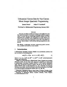
Figure 2.1: The top left picture shows an unbounded convex function without minima, the top right one shows a strictly convex function with a unique minimum, the bottom left one is a non-convex function and the bottom right one is a convex function with infinitely many minima. define y := x − t. We have that (x − y)> (∇f (x) − ∇f (y)) > 0 since f is strictly convex. By inserting the gradients we see that this is equivalent to t> Qt > 0. Furthermore, for a quadratic function we have the equivalence between strictly and uniformly convex. Lemma 2.15. A quadratic function f is strictly convex if and only if f is uniformly convex. Proof. Let λmin be the smallest eigenvalue of Q. We have λmin > 0, such that s> ∇2 f (x)s = 2s> Qs ≥ 2λmin ||s||2 for all s ∈ Rn . In particular Theorem 2.12 implies that any strictly convex quadratic program has a unique minimizer. The following theorem shows that any unconstrained nonconvex quadratic optimization problem is unbounded, while any strictly convex quadratic optimization problem has a unique minimizer that can be computed by solving a system of linear equations. A convex but not strictly convex quadratic optimization problem might have either infinitely many or no minima. In Figure 2.1, we illustrate the different cases for convex functions.

16


Theorem 2.16 ([70]). For UQP, it holds (i) x? is a local minimizer of UQP, if and only if Q is positive semidefinite and ∇f (x? ) = 2Qx? + c = 0. (ii) UQP has a unique solution, if and only if Q is positive definite. (iii) If Q is not positive semidefinite, then UQP is unbounded from below.

2.4.2

Quadratic Programming with Linear Constraints

We consider equality constrained quadratic programming problems, i.e., problems of the form min x> Qx + c> x + d s.t. Ax = b x ∈ Rn ,

(EQP)

where Q ∈ Rn×n , Q = Q> , c ∈ Rn , d ∈ R, A ∈ Rp×n and b ∈ Rp . Equality constrained quadratic programming problems are easy to solve if Q is assumed to be positive semidefinite since this implies f to be convex, and hence the KKTconditions are necessary and sufficient for optimality. Thus, if there exists a solution (x? , µ∗ ) ∈ Rn × Rp of the KKT-system, x? is also a minimizer of EQP, and vice versa. In particular, in this case the KKT-system is a system of linear equations: 2Q A> x −c = . (2.8) A 0 µ b From a practical point of view we have the following theorem. Theorem 2.17 ([91]). Let xk ∈ Rn be feasible for EQP. A pair (x? , µ∗ ) ∈ Rn ×Rp is a KKT-point of EQP if and only if x? = xk + ∆x? and (∆x? , µ∗ ) is a solution of the following system of linear equations 2Q A> ∆x −∇f (xk ) = . A 0 µ 0 This result will be used in standard active set methods, see Section 2.5.3. Concerning the existence and uniqueness of minima for EQP, we can state the following result. Theorem 2.18. If Q is positive definite and rk(A) = p ≤ n, there exists a unique solution (x? , µ∗ ) of (2.8) and x? is the unique minimizer of EQP.

2.4. QUADRATIC PROGRAMMING

17

Proof. Let f be the quadratic objective function of EQP. For any arbitrary vector z ∈ Rn the level sets Nf (z) = {x ∈ Rn | f (x) ≤ f (z)} of f are compact. Since rk(A) = p, we have that the feasible region is nonempty: let A = (A0 , A1 ), where A0 ∈ Rp×p , A1 ∈ Rp×(n−p) and rk(A0 ) = p (if necessary after permutation of the columns of A). Thus, > z0 = (A−1 0 b, 0) is a feasible point. According to Theorem 2.1 there exists a minimizer of EQP. Since f is strictly convex, it is also unique using Theorem 2.12. Again, like in the unconstrained case, it is sufficient to assume the objective function to be strictly convex and additionally the constrained matrix to be fullranked to have a unique solution. Solving the KKT-system (2.8) can be done in different ways. Besides solving it directly, it can be done by using Range-Space Methods or Null-Space Methods. We refer to [162] for details. If we allow inequality constraints, the problem becomes min f (x) := x> Qx + c> x + d s.t. Ax ≤ b x ∈ Rn ,

(QP)

where Q ∈ Rn×n , Q = Q> , c ∈ Rn , d ∈ R, A ∈ Rm×n and b ∈ Rm . By using the necessary optimality conditions (2.5) for NLP and taking into account that no constraint qualification is needed since all constraints are affinelinear [91], we get the following first-order necessary condition for QP. Theorem 2.19 ([162]). If x? is local minimizer of QP, then there exists (x? , λ∗ ) that satisfies the KKT-system: X

2Qx? + c +

λ∗i ai = 0

(Stationarity)

i∈A(x? )

gi (x) =

? a> i x ? a> i x

≤ bi , i ∈ N (x? ) ?

gi (x) = = bi , i ∈ A(x ) ∗ λi ≥ 0, i ∈ A(x? ) λ∗i = 0, i ∈ N (x? )

(Primal Feasibility) (Primal Feasibility) (Dual Feasibility, Complementarity) (Dual Feasibility, Complementarity)

Again, Theorem 2.12 and Lemma 2.15 imply the existence of a unique solution if Q is positive definite. Corollary 1. If Q is positive definite and the feasible region is nonempty, then there exists a unique solution for QP.

18


In this case, since the KKT-conditions are necessary and sufficient for optimality, we can conclude that the unique minimizer can be computed by the unique solution of the KKT-system. For general Q, we can at least give sufficient conditions under which there exists a minimizer. The result is the well-known theorem of Frank and Wolfe. Theorem 2.20 (Frank-Wolfe Theorem [70]). Let X ⊆ Rn be a nonempty polyhedron, then the optimization problem min{f (x) = x> Qx + c> x + d | x ∈ X} attains its global minimum on X, if and only if f is bounded from below. This theorem is not valid for arbitrary nonlinear functions. For example f (x) = ex does not have any minimizer although bounded from below. Using the FrankWolfe Theorem, it is possible to derive a sufficient condition for the existence of minima for QP, if Q is positive semidefinite but not definite. For any convex set C ⊆ Rn its recession cone is defined as the following cone rec(C) := {y ∈ Rn | x + λy ∈ C for all x ∈ C, λ ≥ 0}. Theorem 2.21 ([58]). Let C ⊆ Rn be the nonempty feasible polyhedral region of QP. Then it holds: (i) If QP has a solution, then x> Qx ≥ 0 for all x ∈ rec(C) and c> x ≥ 0 for all x ∈ rec(C) ∩ ker(Q).

(2.9)

(ii) If (2.9) holds and f is convex, QP has a solution. Without loss of generality assume the polyhedral set contains only inequalities. Otherwise the equations can be written as inequalities. It is interesting that the condition (2.9) can be checked in polynomial time by solving the following linear program: min{c> x | Ax ≤ 0, Qx = 0, x ∈ Rn },

(2.10)

since the recession cone of a polyhedron P = {x ∈ Rn | Ax ≤ b} is the set {x ∈ Rn | Ax ≤ 0}. Thus, if there exists an optimal solution x? of (2.10), such that c> x? < 0, QP is unbounded from below and there is no solution. On the other hand, if c> x? ≥ 0, the objective function is bounded from below and hence there exists at least one solution to the problem if f is convex. This shows that if Q is positive semidefinite (but not positive definite), we have a necessary and sufficient condition for the existence of an optimal solution for QP, which can be checked in polynomial time. In general, there are two common approaches for solving QP, namely interior point methods and active set methods. In interior point methods, a sequence

2.5. METHODS FOR NONLINEAR PROGRAMMING

19

of parameterized barrier functions is (approximately) minimized using Newton’s method. The main computational effort consists in solving the Newton system to get the search direction. In active set methods, at each iteration, a working set that estimates the set of active constraints at the solution is iteratively updated. They will be briefly described in the next Section.

2.5

Methods for Nonlinear Programming

This chapter is based on the books of Nocedal and Wright [162], Bazaraa et al. [17] and Geiger and Kanzow [91] which give a detailed insight into theory and practice of nonlinear optimization. For an overview of NLP software we refer to the work of Leyffer and Majahan [139]. We start with unconstrained optimization problems. They are of great interest since they are often used to solve subproblems in approaches for constrained optimization problems. After giving a brief description of the common approaches, we take a closer look at line search methods. After that, we concentrate on two quadratic programming algorithms, namely the conjugate gradient method for unconstrained convex quadratic programming problems and the active set method for linearly constrained convex quadratic programming problems. All three types of algorithms, line search method, conjugate gradient method and active set method will play an important role in the design of our fast active set algorithm for convex mixed-integer programming in Chapter 5. Finally we take a look at the Frank-Wolfe Algorithm for solving constrained convex optimization problems. We use an algorithm tailored to our branch-and-bound algorithm for a class of mixed-integer portfolio optimization problems in Chapter 7.

2.5.1

Unconstrained Nonlinear Optimization

All algorithms for unconstrained nonlinear optimization problems follow the idea of generating a sequence of iterates {xk }∞ k=0 such that for some iterate we can either verify optimality (up to a certain accuracy) or no progress can be made. The design of these algorithms differs in the way of deciding how to move from one iterate xk to the next xk+1 . There are mainly two categories of approaches of choosing the next iterate: line search methods and trust region methods. Line search methods are moving from the current iterate xk to a new one xk+1 with a better objective function value along some descent direction sk . To decide how far the step size along the descent direction should be they solve an one-dimensional optimization problem: minαk >0 f (xk + αk xk ). This is often done approximately, since solving this subproblem can already be expensive. If we solve the problem to optimality we call it an exact line search, otherwise an inexact line search.

20


Trust region methods are different, as in each iteration k they first approximate f (xk + s) by some (simpler) auxiliary function f¯k (s) and then minimize it locally in a trust region ∆k in which both are similar: min{f¯k (s) | ||s|| ≤ ∆k }.

(2.11)

Typically trust regions are chosen as either balls ∆k = {s ∈ Rn | ||s|| ≤ ∆}, where ∆ > 0, or boxes/ellipsoids. The auxiliary function is usually chosen as a quadratic function of the form f¯k (s) = f (xk ) + ∇f (xk )> s + 12 s> Bk s, where Bk is either the Hessian or an approximation of it. Depending on the ratio of actual and expected k )−f (xk +sk ) , either the solution sk is reduction of the objective function ρk = f (x f¯k (0)−f¯k (sk ) accepted and the new iterate is set to xk+1 = xk +sk or the trust region is modified and the problem is solved again. It is common to reject the step and decrease the trust region if ρk < 0 since it implies the objective function value to become worse in the current iteration. On the other hand if ρk ≈ 1, we can increase the trust region, and if ρk 1, the current trust region is kept. The fundamental question is how to solve the trust region problems (2.11). Well-known algorithms that solve the problem approximately are for example the dogleg method for positive definite Bk , and the two-dimensional subspace minimization for indefinite Bk , a method by Steinhaug, based on the CG Method, if Bk is chosen as the exact Hessian of f . In this section we are not going into further details about trust region methods since they are not needed in our approaches. A survey on trust region methods is given by Dennis and Schnabel [67]. Line Search Methods We start with the definition of a descent direction, i.e., directions in which we can improve our objective function. In fact, moving along any descent direction of f , we can guarantee an improvement of the objective function value. Definition 2.11 (Descent Direction). Let f : Rn → R be differentiable in x ∈ Rn . A vector s ∈ Rn is called a descent direction of f in x if we have ∇f (x)> s < 0. Lemma 2.22 ([9]). Let f : Rn → R be differentiable in x ∈ Rn and s ∈ Rn be a descent direction in x. Then there exists some α > 0, such that f (x + αs) < f (x). This leads to the following iterative procedure, sketched in Algorithm 1. The algorithm starts with an initial guess x0 and determines a feasible descent direction s0 as well as a feasible step size α0 to compute the new iterate x1 := x0 +α0 s0 with a reduced objective function value. This is repeated until a stopping criterion is satisfied. In practice the stopping criterion is ||∇f (xk )|| < ε, where 0 < ε 1.


21

Algorithm 1: Line Search input : differentiable function f : Rn → R output: stationary point x? of f Choose starting point x0 ∈ R. Set k = 0. while ∇f (xk ) 6= 0 do Compute descent direction sk . Compute step size αk > 0, such that f (xk + αk sk ) < f (xk ). Set xk+1 = xk + αk sk , k = k + 1.

The obvious questions are how to determine a suitable descent direction s and an appropriate step size α. Concerning the descent direction it is common to choose s = −B −1 ∇f for some symmetric and regular matrix B. Two specific choices for B are for example B = I or B = ∇2 f (x), if the Hessian is positive definite. The resulting descent directions are called Anti-Gradient and Newton-Direction, respectively. Assuming we are interested in an inexact line search, some common conditions on the step sizes then are: • Wolfe conditions: f (xk + αk sk ) ≤ f (xk ) + c1 αk ∇f (xk )> sk k

k > k

k > k

∇f (x + αk s ) s ≥ c2 ∇f (x ) s ,

(2.12) (2.13)

where 0 < c1 < c2 < 1. Condition (2.12) is also known as the Armijo condition and guarantees a sufficient decrease of the objective function. The second condition (2.13) is the curvature condition that ensures the line search to make reasonable progress since a sufficiently small step size would always satisfy the Armijo condition. Furthermore, it may be the case that some step size that satisfies the Wolfe conditions is not close to a minimizer of φ(α) = f (xk + αsk ). To ensure this, we can require the derivative φ0 (α) to be non-negative such that points far away from the minimizer are excluded by the following additional requirement (2.14). • Strong Wolfe conditions: f (xk + αk sk ) ≤ f (xk ) + c1 αk ∇f (xk )> sk |∇f (xk + αk sk )> sk | ≤ c2 |∇f (xk )> sk |,

(2.14)

22

CHAPTER 2. NONLINEAR PROGRAMMING where 0 < c1 < c2 < 1. A third pair of conditions are the • Goldstein conditions: f (xk ) + (1 − c)αk ∇f (xk )> sk ≤ f (xk + αk sk ) k

(2.15) k > k

≤ f (x ) + cαk ∇f (x ) s ,

(2.16)

where 0 < c < 21 . Again, the first inequality prevents to have a step size too small and the second inequality ensures the sufficient decrease. Often the sufficient decrease condition (2.12) is combined with a backtracking such that we do not need to consider (2.13). It starts with an initial step size and reduces it step by step until the sufficient decrease condition holds, see Algorithm 2. Algorithm 2: Backtracking Line Search input : iterate xk , search direction sk , step size αk output: feasible step size αk Choose αk > 0, ρ, c ∈ (0, 1). while f (xk + αk sk ) > f (xk ) + cαk ∇f (xk )> sk do Set αk = ραk .

If the descent directions and step sizes are chosen appropriately the line search algorithm converges to a stationary point. We therefore define feasible search directions and feasible step sizes. Definition 2.12 (Feasible Search Direction, Feasible Step Size). Let {sk }k , {xk }k and {αk }k be the the sequences of search directions, iterates and step sizes generated by Algorithm 1. The sequence {sk }k is called feasible, if for all {xk }k we have the implication: ∇f (xk )> sk = 0 ⇒ lim ∇f (xk ) = 0. k→∞ k→∞ ||sk || lim

(2.17)

The sequence {αk }k is called feasible, if for all {xk }k and {sk }k we have the implication: f (xk + αk sk ) < f (xk ) for all k ∈ N and ∇f (xk )> sk = 0. k→∞ ||sk ||

lim (f (xk ) − f (xk + αk sk )) = 0 ⇒ lim

k→∞


23

The condition (2.17) ensures that the descent direction does not tend to become orthogonal to the gradient. Both, the Anti-Gradient as well as the NewtonDirection are feasible search directions. On the other hand, it can be shown that under standard assumptions the Wolfe conditions as well as the Goldstein conditions are choosing step sizes that are both feasible. Under additional requirements, we can assure the convergence of the line search method to a minimizer. Theorem 2.23 ([9]). Let f : Rn → R be continuously differentiable, x0 be the starting point, the level set Nf (x0 ) be convex and compact and f strictly convex on Nf (x0 ). Furthermore, let the sequence of descent directions {sk }k and step sizes {αk }k be feasible. Then there exists a unique global minimizer x? of f and Algorithm 1 produces a sequence {xk }k that converges to x? . The assumptions made are quite restrictive since we require the objective function in a neighborhood of x? to be strictly convex and additionally that the starting point x0 has to be in that neighbourhood. One of the most important representatives of line search algorithms is the Newton Method that uses in its most general form the Newton Direction as a descent direction and step size 1. Assuming the starting point x0 is sufficiently close to a minimizer x? , it can be shown that if f is twice continuously differentiable and the Hessian of f is Lipschitz continuous in a neighbourhood of x? at which ∇f (x? ) = 0 and ∇2 f (x? ) is positive definite, then {xk }k converges to x? and {||∇f (xk )||}k converges to 0 quadratically. Several modifications can be made to get a practical global convergent version of the Newton Method. For example in the Modified Newton Method, whenever necessary, the Hessian is modified to be positive definite throughout the whole algorithm to guarantee descent directions. To save computational expenses, the computation of the Newton Direction can be done approximately, yielding an Inexact Newton Method. In particular, QuasiNewton type methods aim at reducing the computational effort by approximating the Hessian with some matrix that is easier to invert.

2.5.2

Unconstrained Quadratic Optimization

Conjugate Gradient Method The conjugate gradient method (CG) was introduced by Hestenes and Stiefel [110] in the 1950s for solving systems of linear equations Qx = b for any positive definite coefficient matrix Q ∈ Rn×n and right hand side vector b ∈ R. It is obvious that solving Qx = b is equivalent to minimizing the unconstrained quadratic programming problem 1 (2.18) min{f (x) = x> Qx − b> x | x ∈ Rn }. 2

24


Looking at this, we can consider unconstrained quadratic programming as an alternative way to solve systems of linear equations, if Q is positive definite. Theorems 2.12 and 2.13 guarantee the existence of a unique minimizer of the quadratic programming problem. CG Methods are specific line search algorithms, i.e., they iteratively create a sequence of points xk+1 = xk + αk sk by choosing appropriate step sizes αk and descent directions sk in each iteration. The method starts with the anti-gradient as an initial descent direction but continues with modified Anti-Gradients such that a certain property, called conjugacy holds for the set of search directions. Definition 2.13 (Q-Conjugacy). A set of nonzero vectors {p0 , p1 , . . . , p` } is called > Q-conjugate for a symmetric positive definite matrix Q ∈ Rn×n , if pi Qpj = 0 for all i 6= j. This property ensures that given an arbitrary starting point x0 ∈ Rn and a set of n nonzero Q-conjugate vectors pi ∈ Rn , i = 0, . . . , n − 1, the iterations xk+1 = xk + αk pk ,

(2.19)

k > k

) p , give a minimizer of (2.18) after at most n iterations. where αk = − ∇fpk(x> Qp k Note that any two eigenvectors of Q corresponding to distinct eigenvalues are Q-conjugate. But computing all the eigenvectors would be too expensive. Instead of computing all the Q-conjugate vectors a priori, it is possible to compute them iteratively. This leads to the question of how to determine a set of Q-conjugate vectors. The answer is given by the following constructive Lemma.

Lemma 2.24 ([90]). Let p0 ∈ Rn , p0 6= 0 be arbitrary and pk , k = 1, . . . , n − 1, be defined by pk = −∇f (xk ) + βk−1 pk−1 , where βk−1 =

∇f (xk )> Qpk−1 pk−1 > Qpk−1

and xk defined as in (2.19). Then p0 , . . . , pn−1 are Q-conjugate. Note that in the above construction of the set of Q-conjugate vectors, each vector xk is constructed by using the current iterate xk and the preceding conjugate vector pk−1 . In practice, the computation of αk and βk can be simplified by the following formulas αk =

||∇f (xk )||2 pk > Qpk

,

βk =

||∇f (xk+1 )||2 . ||∇f (xk )||2

In particular ∇f (xk )> pk = −||∇f (xk )||2 < 0 for all ∇f (xk ) 6= 0 implies that the CG Method in fact belongs to the class of line search methods. The CG Method in its most general form is given by Algorithm 3. Putting these results together, we can state the following convergence theorem.


25

Algorithm 3: Conjugate Gradient Method input : symmetric, positive definite matrix Q ∈ Rn×n , vector b ∈ Rn output: minimizer of f (x) := 12 x> Qx − L> x Choose x0 ∈ Rn , p0 = −∇f (x0 ), set k = 0. while ∇f (xk ) 6= 0 do (xk )||2 Set αk = ||∇f . > k p Qpk Compute xk+1 = xk + αk pk ∇f (xk+1 ) = ∇f (xk ) + αk Qpk βk = pk+1

||∇f (xk+1 )||2 ||∇f (xk )||2 = −∇f (xk+1 ) + βk pk

Set k = k + 1.

Theorem 2.25 ([90]). If Q is symmetric and positive definite, Algorithm 3 terminates after at most n iterations with the unique minimizer of (2.18).

The convergence rate of the CG Method is linear, since we have the following error estimation:

||xk − x? || ≤

!2k p κ(Q) − 1 p ||x0 − x? ||, κ(Q) + 1

(Q) where κ(Q) = λλmax is the condition of the matrix Q. We can see that the conmin (Q) vergence highly depends on the distribution of the eigenvalues of Q. Therefore, in practice CG Methods are often accelerated via Preconditioning: Instead of using the CG Method for the original problem we consider the transformation y = Cx and the resulting problem C −> QC −1 y = C −1 b, where C ∈ Rn×n is non-singular and κ(C −> QC −1 ) is smaller than κ(Q). Some common choice is the Incomplete ˜ > , where Q ≈ L ˜L ˜ > such that L ˜ is sparser than the Cholesky Factorization C = L the matrix in the exact Cholesky factorization. The idea of the CG Method is extendible to general unconstrained nonlinear optimization problems of the form min{f (x) | x ∈ Rn } with an arbitrary continuously differentiable objective function f : Rn → R. Popular versions are for example the Fletcher-Reeves Method and the Polak-Ribiere Method. For details, we refer to [162].

26

2.5.3


Constrained Quadratic Optimization

Essentially two classes of methods have been developed for solving linearly constrained quadratic programs of the form QP, namely active set methods (ASM) (see, e.g., [94, 168]) and interior point methods (IPM) (see, e.g., [95, 152]). For a detailed comparison, we refer to [162]. In this thesis, we will focus on inequality constrained convex problems, i.e., we assume Q to be positive semidefinite. Equality constrained quadratic programs of the form EQP do not require special algorithms to be solved, since solving its KKT-system, which is a system of linear equations, is sufficient (see Section 2.4). We therefore concentrate on quadratic programs with inequalities and describe a solution technique based on the reduction to equality constrained problems. Active Set Methods The main idea of active set methods is to solve a sequence of equality constrained quadratic programs by considering only the active constraints at the current iterate. For sake of simplicity, assume we have an optimization problem of the form QP without equations, i.e., m = 0. Recall that by Definition 2.3 the active and non-active sets at some point xk are denoted by k A(xk ) := {i | a> i x = bi }

and

N (xk ) := {1, . . . , m} \ A(xk ).

It is well known that active set methods are preferable to interior point methods in practice, if the number of constraints is small or medium. The basic idea of general active set methods for convex quadratic programming problems relies on the following observation. If x? is the minimizer of QP, we have x? = argmin f (x) s.t. Ax ≤ b ? = argmin f (x) s.t. a> i x = bi for all i ∈ A(x ).

Knowing the optimal active set of x? would solve the problem immediately by finding the solution to (2.8). Since this is not the case, the approach starts by choosing a working set Wk ⊆ {1, . . . , m} and computing xk+1 = argmin f (x) s.t. a> i x = bi for all i ∈ Wk . If the new iterate xk+1 is not the minimizer of QP, adjust Wk to Wk+1 in a clever way and solve the updated equality constrained quadratic programming problem. It is common to distinguish between primal and dual active set methods. While a primal active set method ensures primal feasibility of all iterates, a dual active set methods ensures dual feasibility.


27

Let Wk denote the current working set and Ak the matrix that consists of all rows of A belonging to Wk . We assume that the row vectors ai , i = 1, . . . , m, are linearly independent. Algorithm 4 gives a basic version of a primal active set method for quadratic optimization problems with linear inequalities. Theorem 2.26 ([91]). Consider Algorithm 4 for Problem QP. (i) If Q is positive definite and ai (i ∈ Wk ) are linear independent, (2.20) has a unique solution. (ii) If ai (i ∈ Wk ) are linear independent at any iteration k and the algorithm does not terminate after solving (2.20), this also holds for ai (i ∈ Wk+1 ). (c) If Q is positive definite and ∆xk 6= 0, we have ∇f (xk )> ∆xk < 0, i.e., ∆xk is a descent direction. In each iteration k, the algorithm considers the feasible iterate xk and checks if it minimizes the quadratic objective function in the subspace defined by the current working set Wk . If not, it computes a descent direction ∆xk by solving (2.20). This corresponds to solving the equality constrained quadratic program with constraints a> i x = bi for all i ∈ Wk while all other constraints are relaxed. From Theorem 2.17 we know that ∆xk 6= 0, since otherwise the iterate would already be optimal in that subspace. On the other hand (xk + ∆xk , λk+1 Wk ) is a KKT-point k of that equality constrained problem. Since Ak ∆x = 0, every constraint in the working set will still be satisfied with equality by the new iterate xk + ∆xk . If (c) holds, i.e., xk + ∆xk is feasible for all constraints, we update our iterate and the working set is not changed. If there are constraints i ∈ / Wk that are violated by the new iterate, we choose the step size αk as large as possible until the first constraint that is violated becomes active and any other constraints stays strictly k bi −a> i x feasible. Therefore we choose the step size as αk := mini∈W k >0 > ∆xk , / k , a> ∆x a i i

update our iterate by xk + αk ∆xk and add this blocking constraint to the working set. This iterative process is repeated until a point is reached that is optimal for the current working set, i.e., when ∆xk = 0. Then, either all of the multipliers in the working set Wk are non-negative and we can stop since (xk+1 , λk+1 ) is already a KKT-point of our original problem, or if there is a negative multiplier in the working set Wk , we remove this constraint. It can be shown that the solution of the resulting subproblem (2.20) gives a feasible direction for the constraint that has just been dropped. Assuming that it is always possible to take a nonzero step along a nonzero descent direction guarantees that the algorithm does not cycle. It can also be shown that no working set is considered twice. Since the number of different working sets is finite, the algorithm stops after a finite number of iterations with a KKT-point of the problem. Nevertheless active set methods can have exponential running time

28


Algorithm 4: Active Set Method input : symmetric, positive definite matrix Q ∈ Rn×n , matrix A ∈ Rm×n , vectors c ∈ Rn , b ∈ Rm output: minimizer of q(x) := x> Qx + c> x such that Ax ≤ b 0 Choose feasible x0 ∈ Rn for QP and λ0 ∈ Rm . Set W0 := {i | a> i x = bi }.

while (xk , λk ) is not a KKT-point do Set λk+1 := 0 for all i ∈ / Wk . Solve i ∆x −∇f (xk ) 2Q A> k = . A> 0 λA 0 k

(2.20)

Distinguish between: (a) If ∆xk = 0 and λk+1 ≥ 0 for all i ∈ Wk : STOP i (b) If ∆xk = 0 and min{λk+1 | i ∈ Wk } < 0: i choose q := arg min{λk+1 | i ∈ Wk } i and set xk+1 := xk , Wk+1 := Wk \ {q}. (c) If ∆xk 6= 0 and xk + ∆xk is feasible for QP: set xk+1 := xk + ∆xk , Wk+1 := Wk . (d) If ∆xk 6= 0 and xk + ∆xk is infeasible for QP: choose k b i − a> i x > k |i∈ / Wk s.t. ai ∆x > 0 r := arg min k a> i ∆x and set k b r − a> r x , k a> r ∆x := xk + αk ∆xk , := Wk ∪ {r}.

αk := xk+1 Wk+1 Set k := k + 1.


29

in the dimension of the problem [125], due to the existence of up to 2n possible working sets, but their practical performance is usually much better. A significant advantage of active set methods is that they can be easily warmstarted. We will profit from this fact in the design of our branch-and-bound algorithms.

2.5.4

Constrained Nonlinear Optimization

There are plenty of classical and well-studied approaches for solving constrained, but not necessarily convex, nonlinear optimization problems. We give a short overview without going into detail. At the end we focus on the Frank-Wolfe method that will be use in the last chapter of this thesis. Penalty Methods follow the idea of replacing the constrained problem by a sequence of unconstrained optimization problems Pk := min{f (x)+τk P (x)}, where P (x) is a non-negative penalty function that is zero if and only if x is feasible and τk > 0 is a positive penalty parameter. The use of penalty function and parameter ensures that the objective function is penalized by a perturbation if x is infeasible. The magnitude of perturbation for each unconstrained problem Pk is controlled by the parameter τk . For a strictly monotonically increasing sequence of penalty parameters {τk }k it can be shown that for suitable penalty functions every limit point of the sequence of minimizers {xk }k solves the originalP constrained problem. τk τ 2 2 Typically Pk is chosen as Pk := min{f (x) + 2 ||h(x)|| + 2 m i=1 max {0, gi (x)}}. Penalty Methods usually suffer from the fact that Pk becomes ill-conditioned for growing τk . Exact Penalty Methods overcome this disadvantage by considering a bounded sequence of penalty parameters. Exact penalty functions have the property that there exists τk¯ > 0, such that if x? is a minimizer of f , it is also a minimizer ¯ This makes it possible to tackle the problem by solving of Pk¯ for every k ≥ k. a single (or at least a small number of) unconstrained problem(s) instead of a whole sequence. The penalty functions Pq (x) := f (x) + τ ||(h(x), max{0, g(x)})||q , q ∈ [1, ∞), are standard choices in practice. It is known that Pq , q ∈ [1, ∞), is exact for convex optimization problems while they are even exact for general nonlinear optimization problems if in addition x? satisfies a constraint qualification. The disadvantage of exact penalty functions is that they are necessarily non-differentiable and methods of non-differentiable optimization, like the bundle method, are needed. A popular reference on non-differentiable methods, especially on bundle methods, is given by [124]. Barrier Methods for inequality constrained problems use a similar strategy. Again a sequence of unconstrained problems is considered. In contrast to Penalty Methods they compute a sequence of feasible instead of infeasible iterates by using barrier terms that keep the iterate in the interior of the feasible region. The barrier term is chosen in a way that it penalizes the function only if the iterate

30


is moving towards the boundary of the feasible region. For example logarithmic barrier terms are often used, resulting in unconstrained problems of the form Pm Bk := min{f (x) − τk i=1 ln(−gi (x))}. In this case, we solve Bk for a strictly monotonically decreasing sequence of barrier parameters τk > 0 and every limit point of a sequence {xk }k generated by a Barrier Method is a global minimizer of the original constrained problem. Unfortunately, Barrier Methods also suffer from ill-conditioned problems when τk is converges to zero from above. Augmented Lagrangian Methods, also known as Multiplier-Penalty Methods, combine Lagrangian multipliers with penalty functions. For constrained nonlinear programming problems the augmented Lagrangian can be chosen as Pm function 1 τ 2 > 2 La (x, λ, µ, τ ) := f (x) + 2 ||h(x))|| + µ h(x) + 2τ i=1 (max {0, λi + τ gi (x)} − λ2i ), which is a continuously differentiable function. It can be shown that there exists τ¯ > 0 such that any strict local minimizer x? of f is also a strict local minimizer of La (x, λ∗ , µ∗ , τ ) for all τ ≥ τ¯, where (λ∗ , µ∗ ) are the optimal Lagrangian multipliers. Since neither τ¯ nor (λ∗ , µ∗ ) are known a priori, one usually uses iterative procedures to approximate (λ∗ , µ∗ ) and τ¯ in each iteration. In general, Augmented Lagrangian Methods tend to be less vulnerable to ill-conditioning of the generated subproblems. Sequential Quadratic Programming (SQP) Methods are among the most popular methods for constrained nonlinear programming problems. Their essential idea is to successively model the problem at each iterate xk by a quadratic programming problem and use its solution to define the new iterate xk+1 . SQP Methods can be seen as an application of the Newton Method to the KKT-system and are therefore sometimes also called Newton-Lagrange Methods. To be more precise each iteration k consists of solving the quadratic program 1 > 2 s ∇xx L(xk , λ, µ)s + ∇f (xk )s 2 s.t. ∇hi (xk )> s + hi (xk ) = 0, i = 1, . . . , p

min

∇gj (xk )> s + gj (xk ) = 0, j = 1, . . . , m, and setting xk+1 = xk + s. This quadratic model consists of a quadratic approximation of the Lagrangian and a linear approximation of the constraints. It can be solved by using standard methods of constrained quadratic programming. Additional strategies inspired by line search and trust-region methods can be used to ensure global convergence from an arbitrary starting point, yielding a very effective instrument to tackle constrained nonlinear programs. In Chapter 7, we will deal with convex but not necessarily quadratic mixedinteger problems. To solve their continuous relaxations effectively we rely on the following classical method from convex optimization.


31

Frank-Wolfe Algorithm The Frank-Wolfe Algorithm, also known as the Conditional Gradient Method [85] was proposed in 1956 by Marguerite Frank and Philip Wolfe to originally solve convex quadratic optimization problems over a polygonal set and can be extended to convex problems of the more general form CP. This method was in fact one of the breakthroughs in convex optimization. It assumes that the problem: min{c> x | x ∈ C} can be solved effectively for any linear objective function c> x. We assume C to be compact, nonempty and f to be continuously differentiable. Again, the FrankWolfe Algorithm can be categorized as a line search method. In each iteration, the search direction is computed by solving a convex problem with a linear objective function. In case C is a polygonal region this is just a linear programming problem. The main idea is to replace the general convex objective function f by its first-order Taylor approximation. More precisely, given an iterate xk ∈ C, we consider the Taylor expansion of f about xk : f (xk ) + ∇f (xk )> (y − xk ) and minimize it over the feasible region C. Since f (xk ) and ∇f (xk )> xk are constant, we can replace the objective function by lk (y) = ∇f (xk )> (y − xk ), yielding the following subproblem that has to be solved in each iteration k: min{∇f (xk )> y | y ∈ C}.

(F Wk )

Let y k denote the minimizer of F Wk . Then y k − xk is a feasible direction. Moreover it is a descent direction. To see this, note that the variational inequality ∇f (y k )> (y − y k ) ≥ 0 for all y ∈ C is a sufficient condition for y k to be a minimizer of f over C. Since y k is the minimizer of F Wk , we have lk (y k ) ≤ lk (xk ) = ∇f (xk )> (xk − xk ) = 0. This means that lk (y k ) is either zero or negative. In the first case, we have 0 = lk (y k ) ≤ lk (y) = ∇f (xk )> (y − xk ) for all y ∈ C, meaning that xk is already stationary and we can stop. In the second case we have 0 > lk (y k ) = ∇f (xk )> (y k − xk ), implying sk := y k − xk to be a descent direction. We can improve our iterate by moving along sk with any step size αk ≤ 1, by the convexity of f . Some possible choices for the step sizes are:

32

CHAPTER 2. NONLINEAR PROGRAMMING • an exact step size αk := arg minα f (xk + αdk ) • an Armijo Rule, compare (2.12) • a constant step size αk = 1. • the simple step size αk =

2 . k+2

Assuming C to be compact, the existence of a limit point x¯ ∈ C is guaranteed and we can derive the following convergence theorem: Theorem 2.27 ([26]). Let {xk } be as sequence generated by the Frank-Wolfe Algorithm: xk+1 = xk + αk sk . If all step sizes αk satisfy (a) f (xk+1 ) < f (xk ), if ∇f (xk ) 6= 0, (b) If ∇f (xk ) 6= 0 for all k, then ∇f (xk )> sk = 0. k→∞ ||sk || lim

Then every limit point x¯ of {xk } is a stationary point. In Algorithm 5 we sketch the basic scheme of the Frank-Wolfe Algorithm. The Algorithm 5: Frank-Wolfe Algorithm input : convex function f : Rn → R and convex set C ⊆ Rn output: minimizer of f (x) such that x ∈ C Set k = 0, choose xk ∈ C. repeat Solve z k := min{∇f (xk )> y | y ∈ C}. Let y k be the minimizer. if (z k < 0) then Set sk := y k − xk . Choose αk ≤ 1 using any step size rule. Set xk+1 = xk + αk sk and k = k + 1. until z k = 0 STOP: xk is a stationary point. Frank-Wolfe algorithm is widely used for sparse greedy optimization in machine learning and signal processing problems. An overview about the history and recent variants of this algorithm is given in [115].

Chapter 3 Convex Mixed-Integer Nonlinear Programming In this chapter we are concerned with the solution of convex integer nonlinear optimization problems, i.e., problems of the form INLP, where f and g are assumed to be convex. The reason for considering convex mixed-integer optimization problems is that their continuous relaxation is a pure continuous convex problem, that can be handled effectively because of its good properties, see Section 2.3.2. Indeed, considered as a breakthrough in convex optimization, Nemirovski and Nesterov [161] showed that interior point methods can be used to solve convex optimization problems to a given accuracy with a number of operations that does not grow faster than a polynomial of the problem dimension. Special classes include linear programming (LP), second order cone programming (SOCP) and, under reasonable assumptions, also semidefinite programming (SDP). We note that many convex optimization problems can be cast as one of these. For modern interior point methods in convex optimization, we refer to the book of Ben-Tal and Nemirovski [20]. On the contrary, for many non-convex optimization problems, in the worst case, all known algorithms require a number of operations that is exponential in the problem dimension, e.g., global quadratic optimization is already NP-hard [173]. In fact all algorithms for solving mixed-integer nonlinear programming problems are based on the solution of subproblems which are either integer linear programming (ILP) problems or continuous nonlinear programming (NLP) problems, as we will see in Section 3.2. In both cases the underlying subproblem should be easier to solve than the original problem. Therefore convexity is crucial to tackle the NLP problems. It is also worth to mention that convexity is often used to deal with non-convex problems, especially for computing dual bounds, e.g., in the context of branchand-bound. This is often done by convexifying the constraints or using Lagrangian relaxation that is always a convex optimization problem. A detailed survey about non-convex mixed-integer nonlinear programming is given by Burer and Letch33

34

CHAPTER 3. CONVEX MIXED-INTEGER PROGRAMMING

ford [45]. We will not discuss any problems with non-convexity besides integrality in this work. To motivate integer programming, let us consider the following two dimensional integer linear optimization problem, taken from [191]. Example 3.1. max 1.00x1 + 0.64x2 s.t. 50x1 + 31x2 ≤ 250 3x1 − 2x2 ≥ −4 x1 , x2 ≥ 0 x1 , x2 ∈ Z This integer linear optimization problem has the optimal solution x¯? = (5, 0)> . If 376 950 > we relax the integrality restriction on x, i.e., to x ∈ R2 , we get x¯ = ( 193 , 193 ) as the optimal solution of the LP-relaxation. Intuitively, one might think of rounding the continuous minimizer to obtain the optimal integer solution. In our small example this does not help since rounding the components of x¯ to the nearest integer gives xˆ = (2, 5)> which is first of all far away from the optimal integer solution but also infeasible, while rounding x¯ to the nearest feasible point gives x˜ = (2, 4). Figure 3.1 illustrates this problem. Unless the underlying optimization problem has a special structure, rounding does not give an optimal integer solution. Although in general it is not true, there exist special classes of optimization problems where clever rounding of the LP-solution gives the optimal integer solution [112]. This small motivating example gives rise to the question how we can design algorithms to handle integrality and solve integer optimization problems to optimality. We start this chapter with a section about Mixed-Integer Linear Programming problems, i.e., we assume f and g to be linear. After introducing the machinery to deal with such kind of problems, we continue with convex but nonlinear functions f and g and explain how theory and algorithms for the linear case can be adapted and used for convex Mixed-Integer Nonlinear Programming.

3.1

Basic Methods for Mixed-Integer Linear Programming

If in MINLP, we require both the objective function f and the constraints g to be linear, it reduces to a Mixed-Integer Linear Program: min {c> x + d> y | Ax + By ≤ b, x ∈ X ∩ Zn , y ∈ Y },

(MILP)

3.1. MIXED-INTEGER LINEAR PROGRAMMING

35

y

cont. min.

2y + x ≤ 10

x c = (1.00, 0.64)> Figure 3.1: The feasible region of the LP-relaxation (blue lines), the integer feasible points (red dots) and its convex hull (red lines), the continuous minimizer x¯ = (376/193, 950/193)> (blue dot), the integer minimizer x? = (5, 0)> (yellow dot), a cutting plane (orange dashed line) and the level set {x ∈ R2 | c> x = 5} (black dashed line). where c ∈ Rn , d ∈ Rp , A ∈ Rm×n , B ∈ Rm×p , b ∈ Rm and X ⊆ Rn , Y ⊆ Rp are polyhedra. Integer linear programming is known to be NP-hard. In the last decades mainly two algorithmic approaches have been developed to handle integer linear and also nonlinear programming problems: branch-and-bound [59, 132, 144], cutting planes [63, 96, 97] and branch-and-cut [164] as a mixture of both. In nearly every state-of-the-art software at least one of these approaches is implemented. We refer to [159, 175, 191] for a comprehensive overview in the theory of mixedinteger linear programming. Surveys about software for solving mixed-integer linear programming problems are given by [141, 142, 145].

3.1.1

Branch-and-Bound Algorithm

Mixed-Integer Linear Programming problems are generally solved using a linear programming based branch-and-bound algorithm. This is due to the fact that linear programming problems can be solved efficiently in theory by the ellipsoid method [123] as well as by the interior point method [120]. In practice

36


linear programming problems are solved effectively, since the Simplex Algorithm was introduced by Dantzig in late sixties [62]. Basic LP-based branch-and-bound is nowadays used in nearly every state-of-the-art MIP software. The main idea of branch-and-bound is based on the concept of relaxations. Instead of solving the original mixed-integer programming problem, we remove all integrality restrictions, resulting in a linear programming problem, called the LP-relaxation, usually also known as the continuous relaxation of the original mixed-integer problem. More generally, relaxing the integrality condition x ∈ Zn in an integer nonlinearoptimization problem INLP results in a problem of the form NLP, i.e., a continuous optimization problem that can be handled by algorithms for nonlinear optimization problems. In particular if the underlying problem is convex it is likely that we can find an efficient algorithm to solve the subproblem. In this way, we obtain a lower bound on the optimal objective function value of the mixed-integer problem. More generally, there are many ways to compute lower bounds for mixed-integer nonlinear programming problems by using the concept of relaxation. To be more precise, a relaxation is defined as follows. Definition 3.1 (Relaxation). For a given minimization problem f ∗ := min{f (x) | x ∈ F}

(P)

we call the optimization problem ¯ f¯∗ := min{f¯(x) | x ∈ F}

(R)

a relaxation for P, if the following two conditions hold: (i) F ⊆ F¯ and (ii) f¯(x) ≤ f (x), for all x ∈ F. There are two possibilities to relax an optimization problem. The first one is to enlarge the feasible set F, the second one is to find an underestimator for the objective function, such that it always has a value less or equal than the original one. Of course, one is interested in finding relaxations which are easy to solve, but are also close to the original problem. Since there is no need to simplify f , the first possibility is more promising in our case. It follows directly that solving a relaxation always gives a lower bound on f ∗ = f (x? ). During the branch-andbound process, the following properties hold: (P1) For any relaxation R of P, we have f¯∗ ≤ f ∗ . (P2) If any relaxation R of P is infeasible, P is also infeasible. (P3) If for any relaxation R of P we have f¯∗ = f ∗ , then x? is also optimal for P. On the other hand, we observe that for any feasible x ∈ F, f (x) gives an upper bound on f ∗ . The goal in branch-and-bound will be to find good lower and upper bounds on f ∗ .


37

Algorithm 6: LP-based branch-and-bound for MILP input : Polyhedron P = {(x, y) ∈ X × Y | Ax + By ≤ b}, c ∈ Rn output: min c> x s.t. (x, y) ∈ P ∩ (Zn × Rp ) Set P = {(x, y) ∈ X × Y | Ax + By ≤ b}, L = {P }, U = ∞. while L 6= ∅ do Choose P ∈ L and set L := L \ {P }. Solve min{c> x + d> y | (x, y) ∈ P }. if (?) is infeasible then Set f ∗ = ∞. else Let (x? , y ∗ ) denote the optimal solution of (?) and set f ∗ = c> x? + d> y ∗ . if f ∗ ≥ U then Continue if (x? , y ∗ ) ∈ P ∩ (Zn × Rp ) then if f ∗ < U then Set (¯ x, y¯) = (x? , y ∗ ) and U = f ∗ . Continue Choose i ∈ {1, . . . , n} such that x?i ∈ / Z and let P1 := {(x, y) ∈ P | xi ≥ dx∗i e} and P2 := {(x, y) ∈ P | xi ≤ bx∗i c}. Set L = L ∪ {P1 , P2 }. if U = ∞ then STOP: The problem is infeasible. else STOP: (¯ x, y¯) is optimal with objective function value U .

(?)

38


Reduced Enumeration by Branching and Bounding Since complete enumeration in combinatorial optimization leads to a combinatorial explosion, meaning that for increasing problem dimension, the number of potential optimal solutions is increasing exponentially in the dimension, we are seeking for some more intelligent algorithms for finding the optimal solution. The basic principle of branch-and-bound is to create a reduced enumeration tree of all feasible candidates by excluding those in advance for which it is known that they cannot be optimal. This can be achieved by using the divide and conquer strategy combined with a Bounding procedure: the original problem P is divided into k more restrictive subproblems P1 , . . . , Pk such that F=

k [

Fi ,

i=1

where F, F1 , . . . , Fk are the feasible sets of P , P1 , . . . , Pk , respectively. Usually the union is chosen to be disjunct. It is clear that z = min{zi , . . . , zk }, where z is the optimal objective function value of P and zi is the optimal objective function values of Pi for all i = 1, . . . , k. In other words the sets of feasible solutions form a (disjunctive) union of the original set of feasible solutions. Since this leads to k different branches in the tree, we call this step Branching. Every subproblem created in this way is called a node in the branch-and-bound tree. The original mixed-integer problem is therefore called the root node. In Algorithm 6, we describe an LP-based branch-and-bound scheme, where the number of subproblems generated at each node is two. This formulation was proposed by Dakin [59] in 1965 and that way of branching is known as dichotomy branching. Every time we find a feasible mixed-integer solution this is a valid upper bound for the optimal objective function value z. On the other hand every relaxation yields a lower bound. We have the following observation. If z¯k and z k denote the upper and lower bound on zk , respectively, we can conclude that z¯ = mink z¯k is an upper bound on z. Therefore we can successively compare upper and lower bounds to potentially exclude branches of the tree. If no upper bound is known at the root node, it is set to infinity. Usually the expressions primal bound and dual bound are used instead of upper and lower bounds to be consistent if switching from minimization to maximization problems. For each subproblem i we solve an appropriate relaxation. Three different cases may occur: (i) the solution is feasible for P . (ii) the solution is feasible for Pi but not feasible for P .


39

(iii) Pi is infeasible. Everytime case (i) occurs, we have found a feasible solution to the original mixedinteger problem and according to property (P2) it is not necessary to continue branching on this node. This is due to the fact that in every consecutive node, originating from the current one, the objective function value is non-decreasing since we restrict the set of feasible solutions. We further check if the solution provides an improved solution, i.e., it has a better objective function value than the best one known so far. If so, it yields an improved primal bound and we update our best solution. For any upcoming node we know that we will never have to accept a feasible mixed-integer solution of value worse than our best primal bound. Otherwise, if we do not get an improved solution, we simply proceed with the tree search. If case (ii) occurs, we use the fact that every relaxation yields a dual bound. We can compare it to the best primal bound found so far. Now, if the dual bound is greater or equal to the best known primal bound, we do not need to consider that branch of the tree and therefore cut it off from the search space. This process of comparing dual and primal bounds is known as Bounding. Cutting off a branch is denoted also as Pruning. In the other case, i.e., the dual bound is strictly less than the primal bound, that branch may still contain a better solution and the current subproblems are again divided into k more restrictive ones. This procedure is continued until we either reach a point at which we have solved or pruned all of those subproblems. The best solution at the end is proven to be optimal for the original mixed-integer problem, or if no feasible solution has been found, the problem is infeasible. Finally, if case (iii) occurs, we can prune the node due to property (P3), since there will be for sure no feasible solution for the original problem in that branch. A typical branch-and-bound tree is illustrated in Figure 3.2. To sum up, there are mainly three crucial components that can improve the performance of a generic branch-and-bound algorithm, namely the Branching Strategy, the Node Selection and the Bound Computation. We will shortly discuss the possibilities. Branching Strategies Besides a random branching strategy, where a random fractional variable is chosen, Most-Fractional-Branching is the most intuitive branching strategy, picking some fractional variable in the LP-solution whose distance to the next integer is maximal. In Strong Branching [10] one aims at maximizing the expected increase of the lower bound to prune as early as possible. This is done by solving all nodes originating from branching on each fractional variable. Looking at the optimal objective function value of the current node and comparing it to the solution values of the nodes generated by branching on one of the fractional variables, the branching rule chooses a variable that is promising.

40


xi ≤ bx∗i c

z¯ = 10: new upper bound

xi ≥ dx∗i e .. .

.. .

infeasible .. . z k+1 = 9.5: branch

z k = 10.5: dominated by z¯ .. .

Figure 3.2: Illustration of a branch-and-bound tree using dichotomy branching: the red node indicates the infeasibility of the node relaxation, thus it can be pruned. The green node indicates that a feasible (mixed-)integer solution has been found. In the upper green node a new primal bound of value 10 has been found. In the blue node the dual bound of value 10.5 exceeds the current primal bound and we can also prune, while in the yellow node we need to continue branching.

This strategy requires the exact solution of a lot of nodes at every level of the branching tree. The computational effort can be reduced by solving the nodes only approximately. A similar strategy is devised in [21], called Pseudo-Cost Branching and can be seen as a computationally cheaper version of strong branching. The idea is to replace the exact solution values at the nodes by an estimation of these values, gained from the branchings on that variable done so far in the search tree. Every time a variable has been chosen for branching, the change in the objective function is stored. Then a variable that is predicted to have the biggest change in the objective function based on stored values is chosen. Reliability Branching, introduced by Achterberg et al. [3], combines strong branching and pseudo-cost branching. Since in pseudo-cost branching no data is available for initializing the estimated costs, it is useful to perform strong branching at the beginning, until every variable has been branched on k times, and then switch to pseudo-cost branching. Again the computational effort can be controlled by limiting the number of variables for which strong branching will be executed, if k ≥ 2. For example this can be done by ranking the variables by some score


41

number and taking the best ones. Node Selection Strategies After processing the current node, we have to decide which open node will be processed next. Two common node selection strategies are depth-first search and best-first search. For a fixed branching strategy, depth-first search selects the last node put in the list, which corresponds to the deepest node of the enumeration tree. Best-first search selects the node with the smallest lower bound since it might be more promising to search for the optimal solution in that branch. While a depth-first search leads to a quick initial primal bound, a best-first search might reduce the number of nodes in the enumeration tree. Clearly, on the other hand, depth-first may result in the enumeration of many nodes if no good primal bound can be found quickly while a best-first search might take longer to find any feasible solution before reaching the bottom of the enumeration tree. Both strategies can also be combined in Two-Phase-Methods, e.g., Diving Methods, as proposed in [143]. After starting with a depth-first search, until one or a few feasible solutions have been found, it continues with a best-first search aiming at proving local optimality. Bound Computation Strategies We have to choose which appropriate relaxation for the nodes we want to use to compute the dual bounds. It is intuitive that tighter bounds are more costly to compute but can lead to a smaller overall search tree. In case of an integer linear programming problem it is obvious to use the continuous relaxation. The same trade-off holds for the primal bound. The usage of Primal Heuristics, i.e., algorithms that compute feasible solutions quickly without assuring optimality, can lead to good approximative solutions that can be used as primal bounds to reduce the gap between dual and primal bounds but can be time consuming.

3.1.2

Cutting Plane Algorithm

The motivation of the Cutting Plane Algorithm for mixed-integer linear programming problems comes from a well-known result in integer programming, namely that minimizing a linear function over an arbitrary set is the same when replacing the set by its convex hull: Theorem 3.1 ([191]). Let X ⊆ Rn and c ∈ Rn . Then we have min{c> x | x ∈ X} = min{c> x | x ∈ conv(X)}. In particular, if X = P ∩ Zn , where P is a polyhedron, P 0 := conv(X) is also a polyhedron, i.e., there exists a matrix A˜ and a vector ˜b of appropriate size ˜ ≤ ˜b}. Knowing A˜ and ˜b in advance, would give a such that P 0 = {x ∈ Rn | Ax

42


complete description of the convex hull and in theory such an integer program could be reformulated as a linear programming problem and solved by using any algorithm for linear programming. But in general P 0 might need an exponentially large number of linear inequalities to be described. In practice it is often hard to find an explicit description of P 0 for a set X due to numerical issues, so one is interested in approximating P 0 . The above result is also true for any mixed-integer linear program MILP. The Cutting Plane Algorithm aims at approximating P 0 by the usage of cutting planes. Definition 3.2 (Valid Inequality, Cutting Plane). Let P be a polyhedron and P 0 := conv(P ∩ Zn ). A linear inequality π > x ≤ π0 is a valid inequality for P if it holds for all x ∈ P . A linear inequality is a Cutting Plane for P , if it is valid for P 0 but not for P . In Figure 3.1 a possible cutting plane is shown. There are mainly two reasons why adding cutting planes to P from the beginning is not always reasonable. First, there is generally an exponential number of such additional constraints. Second, by adding additional constraints the LP-relaxations become successively harder to solve. We only want to add these constraints if they are violated by any fractional solution not contained in P 0 . Therefore it is important to study ways of generating cutting planes for P whenever needed. Definition 3.3 (Separation Problem). For a polyhedron P a separation problem is the following problem: Given any x? ∈ Rn , find a valid inequality π > x ≤ π0 for P 0 such that π > x? > π0 or decide that none exists. For any x? ∈ / P 0 , the separation algorithm gives a cutting plane for P . In general, efficient optimization and efficient separation are equivalent, i.e., the following theorem holds: Theorem 3.2 ([191]). For a given class of optimization problems with a linear objective function min{c> x | x ∈ X ⊆ Rn }, there exists an efficient (polynomial) algorithm, if and only if there exists an efficient algorithm for the separation problem associated with the problem class. The main idea of the cutting plane algorithm is to tighten the original formulation of the LP-relaxation by removing undesired fractional solutions during the solution process without the undesired side effect of creating additional subproblems, such as in a branching process. Given the fractional LP solution x? ∈ P found by solving the LP-relaxation, it is tested for being feasible in the integer components. If it is not, the separation problem is solved, i.e., a valid linear inequality for P 0 is determined which cuts off the non-integer point x? . Once such a cutting plane is found, it is added to the LP-relaxation to tighten the feasible set and


43

the relaxation is solved once again. In an iterative fashion, we alternate between adding cutting planes and solving the LP-relaxation with the aim of finding an integer solution. Each time a cutting plane is added, the current feasible set gets closer to the desired convex hull. In Algorithm 7, we sketch a general cutting plane algorithm for problems of the form MILP. It might be the case that Algorithm 7 terminates without finding an integer solution because no further cutting plane can be found. In this case the improved formulation can still be passed to any branch-and-bound algorithm. Algorithm 7: Generic Cutting-Plane Algorithm input : Polyhedron P = {(x, y) ∈ X × Y | Ax + By ≤ b}, c ∈ Rn output: min c> x s.t. (x, y) ∈ P ∩ (Zn × Rp ). repeat Minimize c> x + d> y over P . Let (x? , y ∗ ) ∈ P denote its optimal solution. if x? ∈ Zn then STOP: x? is optimal. else Solve the separation problem for P . if a cutting plane π > (x, y) ≤ π0 is found then Set P := {(x, y) ∈ P | π > (x, y) ≤ π0 }. until no cutting plane was found It remains the question of how to find a cutting plane in Step 3 of Algorithm 7. In the 1950s Ralph Gomory and Vaclav Chvátal independently found out that the following observation holds: Lemma 3.3 ([191]). Given X = PP∩ Zn , where P = {x ∈ Rn | Ax ≤ b, x ≥ 0} n > > and u ∈ Rm + , the linear inequality j=1 bu aj cxj ≤ bu bc is valid for X, where a1 , . . . , an ∈ Rm denote the columns of A ∈ Rm×n . These linear inequalities are known as Chvátal-Gomory Cuts. Adding one of them to P is called the Chvátal-Gomory Procedure. It can be shown that these cuts are sufficient to generate all possible valid inequalities for X. Theorem 3.4 ([191]). Every valid inequality for P ∩ Zn can be obtained by applying the Chvátal-Gomory procedure a finite number of times. The first cutting plane algorithm was introduced by Dantzig, Fulkerson and Johnson in 1954 [63], to solve a 54-city instance of the Traveling Salesman Problem. In 1958 Ralph Gomory [96] formulated an algorithm, based on the Chvátal-Gomory Procedure, for successively generating Chvátal-Gomory Cuts directly out of the

44


optimal simplex tableau for any fractional LP solution found in Step 1, cutting it off. It was the first finite cutting plane algorithm presented for solving general pure integer linear programming problems of the form min{c> x | x ∈ P ∩ Zn }, where P is defined by linear inequalities Ax ≤ b, and A, b are required to be integer valued. Later, in 1960 Gomory [97] introduced the Gomory Mixed-Integer Cuts and extended the algorithm to general mixed-integer linear programming problems. These cuts are based on a disjunctive argument. However, iteratively adding Gomory Mixed-Integer Cuts will only guarantee finite convergence if also the objective function is required to be integer valued. In the last decades, different types of cutting planes have been studied besides the Chvátal-Gomory Cuts and Gomory Mixed-Integer Cuts, e.g., Mixed-Integer Rounding Cuts [150], Lift-and-Project (Disjunctive) Cuts [13, 14], Split Cuts [54], Intersection Cuts [12], {0, 21 }-Cuts [49]. A detailed survey on cutting planes for mixed-integer linear programming is given by Cornuéjols [55]. Their effectiveness depends on the underlying problem and usually different types of cuts are combined. The theory of cutting planes is deep and extensive. It is also generally accepted to be the most important contributor to the computational advances that have been made in integer programming over the last several years. An interesting study by Bixby [31] shows the improvements in solving mixed-integer problems using all innovations over the last decades.

3.1.3

Branch-and-Cut Algorithm

Combining branch-and-bound with the cutting plane algorithm results in the socalled branch-and-cut algorithm and merges the advantages of both approaches. In the root node the LP-relaxation is solved. If the solution is not integer feasible, the separation problem is solved and cutting planes are added to the problem if possible and we repeat as in a cutting plane algorithm. If no cutting plane can be found we switch to a branching procedure as in branch-and-bound. In commonly used optimization software for integer linear programming problems branch-andcut algorithms can be considered as state-of-the-art, see Section 3.3.

3.2

Methods for Convex Mixed-Integer Nonlinear Programming

We are now interested in convex mixed-integer nonlinear programming problems, i.e., problems of the form MINLP: zCM IN LP := min f (x, y) x,y

s.t. g(x, y) ≤ 0 x ∈ X ∩ Zn , y ∈ Y,

(CMINLP)

3.2. CONVEX MIXED-INTEGER NONLINEAR PROGRAMMING

45

where additionally the objective function f , the constraint functions g and the sets X, Y are assumed to be convex. Many optimization problems arising in real world applications can be formulated as convex mixed-integer nonlinear programs of the form CMINLP. Allowing both integrality and nonlinearity makes this class of problems extremely hard. In fact, MINLP comprises the NP-hard subclasses of mixed-integer linear programming (MILP) and general nonlinear programming (NLP). The restriction to convex MINLP preserves NP-hardness, as MILP is still contained as a special case. In literature, there are mainly five approaches for this kind of problems, which we will explain in the following subsections: NLP-based branch-and-bound [105], outer approximation [75, 80], general benders cecomposition [92], extended cutting planes [188] and LP/NLP-based branch-and-bound [169]. A detailed survey of algorithms and software for solving convex MINLP is given by Bonami, Kilin¸c and Linderoth [36]. Especially branch-and-bound and outer approximation will build the main components for our quadratic outer approximation algorithm, presented in Chapter 6. The idea is always to reduce the original problem to a sequence of ILP and/or NLP problems and use the methodology of Chapter 2.

3.2.1

Branch-and-Bound

NLP-based branch-and-bound works analogously to Algorithm 6. Instead of considering its linear programming relaxation, the following nonlinear programming relaxation is used to to compute the dual bounds in Step 4: min f (x, y) x,y

s.t. g(x, y) ≤ 0 x ∈ X, y ∈ Y.

(NLP-R)

This relaxation is also known as the NLP-relaxation of a mixed-integer programming problem. Therefore one may think of choosing any algorithm from nonlinear programming that can solve the continuous relaxation. For this purpose, all algorithms presented in the following chapters make use of one or more algorithms presented in Section 2.5.

3.2.2

Outer Approximation

Outer approximation was introduced by Duran and Grossmann in 1986 [75] and extended to general convex mixed-integer nonlinear programming problems by Fletcher and Leyffer in 1994 [80]. The basic concept is to successively build up a mixed-integer linear programming problem that is equivalent to the original problem by linearizing both the objective function as well as the constraints at

46


y

y

x

x

Figure 3.3: Polyhedral outer approximation of the feasible region (left) and objective function (right).

certain points. Figure 3.3 illustrates an outer approximation of feasible region and objective function. The approach requires the following assumptions: A1 X 6= ∅ is compact. A2 f, g are convex and continuously differentiable. A3 for any fixed integer x¯ ∈ X ∩ Zn , a constraint qualification, e.g., Slater’s condition, holds at the solution of the resulting NLP-relaxation: zN LP (¯x) := min f (¯ x, y) s.t. g(¯ x, y) ≤ 0 y ∈ Y,

(NLP(¯ x))

or, in case NLP(¯ x) is infeasible, at the solution of the following feasibility problem, that minimizes the violation of the constraints g:

zN LP F (¯x) := min

m X

gj (¯ x, y)+

(NLPF(¯ x))

j=1

s.t. y ∈ Y, with gj (¯ x, y)+ := max{0, gj (¯ x, y)}. Introducing a real variable η and using the convexity of f and g, we end up with a mixed-integer linear programming problem for which it can be shown that it is


47

equivalent to CMINLP:. zOA := min η x − x¯ ≤ η, ∀ x¯ ∈ T ∗ s.t. f (¯ x, y(¯ x)) + ∇f (¯ x, y(¯ x)) y − y(¯ x) x − x¯ > ≤ 0, ∀ j = 1, . . . , m, ∀ x¯ ∈ T ∗ gj (¯ x, y(¯ x)) + ∇gj (¯ x, y(¯ x)) y − y(¯ x) (MILP-OA) x − x˜ gj (˜ x, y(˜ x)) + ∇gj (˜ x, y(˜ x))> ≤ 0, ∀ j = 1, . . . , m, ∀ x˜ ∈ S ∗ y − y(˜ x) >

x ∈ X ∩ Zn , y ∈ Y, η ∈ R where T ∗ = {x ∈ X ∩ Zn | NLP(x) is feasible} consists of all integer points in X for which the subproblem is feasible, S ∗ = {x ∈ X ∩ Zn | NLP(x) is infeasible} consists of those for which it is infeasible and y(x) denotes an optimal solution of NLP(x) or NLPF(x), respectively. Theorem 3.5 ([36, 75, 80]). Assuming A1-A3 hold, then zOA = zCM IN LP . All optimal solutions of CMINLP are optimal solutions of MILP-OA. From a practical point of view formulating MILP-OA requires the a priori knowledge of T ∗ and S ∗ , thus also the knowledge of the solutions of all the NLP subproblems for each xk ∈ X ∩ Zn at some iteration k of the outer approximation scheme. Algorithmically, it is therefore convenient to build up the mixed-integer linear problem step by step, alternating between solving the nonlinear programming problem NLP(xk ), yielding a point (xk , y k ) about which we linearize the objective and the constraint functions, and the resulting relaxation MILP-OAk of the mixed-integer linear programming problem MILP-OA at each iteration k:

zOAk := min η x − xh s.t. f (x , y ) + ∇f (x , y ) ≤ η, h ∈ T k y − yh h h h h h > x−x gj (x , y ) + ∇gj (x , y ) ≤ 0, j = 1, . . . , m, h ∈ T k y − yh (MILP-OAk ) x − xl gj (xl , y l ) + ∇gj (xl , y l )> ≤ 0, j = 1, . . . , m, l ∈ S k y − yl h

h

h

h >

x ∈ X ∩ Zn , y ∈ Y, η ∈ R, where T k := {h ≤ k | y h is the optimal solution of NLP(xh )} and analogously S k := {l ≤ k | y l is the optimal solution of NLP(xl )}. It is clear that on the

48


one hand the solution of every feasible problem NLP(xk ) gives a primal bound for CMINLP since it is feasible and on the other hand the solution of MILP-OAk gives an increasing sequence of dual bounds for CMINLP. The iterative procedure stops when primal and dual bounds are within a specified tolerance. Finite convergence is ensured by the following theorem. Theorem 3.6 ([75, 80]). If assumptions A1-A3 hold and |X| < ∞, then Algorithm 8 terminates in a finite number of iterations at the optimal solution of CMINLP or with an indication that it is infeasible. We finally give a sketch of the general outer approximation scheme in Algorithm 8. Note that there exist instances for which Algorithm 8 needs exponentially many Algorithm 8: Outer approximation algorithm input : f : Rn × Rp → R, g : Rn × Rp → Rm convex and differentiable output: min{f (x, y) | g(x, y) ≤ 0, (x, y) ∈ X ∩ Zn × Y } Set k := 0, T k := ∅, S k := ∅, U k := ∞, Lk := −∞ and ε > 0. Choose xk ∈ X ∩ Zn . repeat Solve NLP(xk ) (or NLPF(xk ), if subproblem is infeasible). Let y k be the solution. Linearize f and g about (xk , y k ), set T k+1 := T k ∪ {k} (or S k+1 := S k ∪ {k}, if subproblem is infeasible). if NLP(xk ) is feasible and f (xk , y k ) < U k then Set (x? , y ∗ ) = (xk , y k ) and U k+1 = f (xk , y k ). else U k+1 = U k . Solve MILP-OAk . Let (xk+1 , y k+1 ) be the solution and Lk+1 := zOAk . Set k = k + 1. until U k − Lk < ε STOP: (xk , y k ) is the optimal solution. iterations to converge, see, e.g., [111], meaning we need to solve exponentially many mixed-inter linear programming problems. Figure 3.4, taken from [111], Pn n shows the empty set Bn := {x ∈ {0, 1} | i=1 (xi − 21 )2 ≤ n−1 } as the intersection 4 √ n−1 of the vertices of an n-dimensional hypercube with a ball of radius 2 centered in ( 12 , . . . , 12 ). Algorithm 8 would need 2n iterations to converge, since only one vertex can be cut by an outer approximation constraint in each iteration.

3.2.3

Generalized Benders Decomposition

Generalized Benders Decomposition for CMINLP was devised by Geoffrion [92] in 1972, and is very similar to the presented outer approximation algorithm, but


49

Figure 3.4: Worst-case example: exponentially many iterations are needed by outer approximation to detect infeasibility [111]. was proposed earlier. The difference between both approaches is the construction of the mixed-integer linear programming problems for computing the dual bounds. At iteration k, having solved NLP(xk ) with the corresponding solution y k , instead of adding all linearizations of g about (xk , y k ), the idea is to add a cut that turns out to be an aggregation of these linearizations, thus yielding a potentially weaker bound than the one resulting from outer approximation. This is why the majority of available solvers prefer outer approximation to the Generalized Benders Decomposition to solve convex MINLP (see Section 3.3). In [1], Abishek, Leyffer and Linderoth use the resulting Benders cuts to aggregate inequalities in their LP/NLP-based branch-and-bound software FilMINT. We will give a brief derivation of the MILP. Again, we require the assumptions A1-A3 on CMINLP and use arguments from nonlinear duality theory. We start with the dual representation of NLP(xk ). According to Definition 2.7 the Lagrangian dual is zDN LP (xk ) := max min f (xk , y) + λ> g(xk , y). m λ∈R+ y∈Y

(DNLP(xk ))

Using assumptions A1-A3 we have that strong duality holds for NLP(xk ), i.e., zN LP (xk ) = zDN LP (xk ) . Thus, we have zCM IN LP = min zN LP (xk ) xk ∈V k = min max min L(x , y, λ) m xk ∈V

λ∈R+ y∈Y

= min{α | α ≥ min L(xk , y, λ) ∀λ ≥ 0, α ∈ R, xk ∈ V }, y∈Y

where V := {x ∈ X ∩ Zn | ∃ y ∈ Y : g(x, y) ≤ 0} is the set of all feasible integer assignments for which there exists a feasible continuous part. Since V is

50


not known explicitly, xk ∈ V has to be reformulated by inequality constraints. This is done by the feasibility problem NLPF(xk ), knowing that xk ∈ V if and only if NLPF(xk ) has a positive minimum. Considering its Lagrangian dual and again using strong duality yields the condition xk ∈ V if and only if m X > k m 0 ≥ min µ g(x , y) for all µ ∈ Λ := {µ ∈ R+ | µi = 1}. y∈Y

i=1

Finally, we get the following MILP which is equivalent to CMINLP zGBD := min η s.t. min L(x, y, λ) ≤ η ∀λ ≥ 0 y∈Y

min µ> g(x, y) ≤ 0 ∀µ ∈ Λ

(MILP-GBD)

y∈Y

x ∈ X ∩ Zn , η ∈ R. Also here, it is not useful to solve this problem directly, since there are infinitely many constraints. By linearization, we get the relaxation min η s.t. L(xh , y h , λh ) + ∇x L(xh , y h , λh )> (x − xh ) ≤ η, h ∈ T k (µl )> g(xl , y l ) + ∇x g(xl , y l )> (x − xl ) ≤ 0, l ∈ S k x ∈ X ∩ Zn , η ∈ R,

(MILP-GBDk )

where T k and S k are defined as for MILP-OAk . Finally we want to show that the cut, added to the mixed-integer linear programming problem, is an aggregation of those in outer approximation. From the KKT-conditions of NLP(xk ) we have ∇y f (xk , y k ) + (λk )> ∇y g(xk , y k ) = 0 k >

k

k

(λ ) g(x , y ) = 0,

(3.1) (3.2)

where (y k , λk ) is the pair of primal and dual solution. The linearizations used in outer approximation are:

k

k

k

k >

k

k

k

k >

f (x , y ) + ∇f (x , y ) g(x , y ) + ∇g(x , y )

x − xk y − yk

x − xk y − yk

≤η

(3.3)

≤ 0.

(3.4)

Using the equations (3.1),(3.2), and adding the inequalities of (3.3),(3.4) where the second one is multiplied by λk yields f (xk , y k ) + ∇x f (xk , y k )> (x − xk ) + (λk )> ∇x g(xk , y k )(x − xk ) ≤ η ⇔L(xk , y k , λk ) + ∇x L(xk , y k , λk )> (x − xk ) ≤ η.


51

Algorithm 9: General Benders Decomposition input : f : Rn × Rp → R, g : Rn × Rp → Rm convex and differentiable output: min{f (x, y) | g(x, y) ≤ 0, (x, y) ∈ X ∩ Zn × Y } Set k := 0, T k := ∅, S k := ∅, U k := ∞. Choose xk ∈ X ∩ Zn . repeat Solve NLP(¯ x) (or NLPF(¯ x), if subproblem is infeasible). Let y k be the solution. Linearize f and g about (xk , y k ), set T k+1 := T k ∪ {k} (or S k+1 := S k ∪ {k}, if subproblem is infeasible). if NLP(¯ x) is feasible and f (xk , y k ) < U k then Set (x? , y ∗ ) = (xk , y k ) and U k+1 = f (xk , y k ). else U k+1 = U k . Solve MILP-GBDk . if MILP-GBDk is feasible then Let (xk+1 , y k+1 ) be the solution. Set k = k + 1. until MILP-GBDk is infeasible STOP: (xk , y k ) is the optimal solution.

These inequalities are also known as Benders Cuts. Since they are aggregations of the cuts from the outer approximation procedure, the resulting dual bounds are weaker. We give a detailed scheme of the algorithm in Algorithm 9 that is identical to outer approximation, except of exchanging the problems MILP-OAk by MILP-GBDk . Analogously we have the following optimality and convergence theorem. Theorem 3.7 ([92]). Assuming A1-A3 hold, then zCM IN LP = zGBD and the algorithm terminates in a finite number of steps at the optimal solution of CMINLP or with an indication that it is infeasible.

3.2.4

Extended Cutting Planes

In 1960, Kelley [122] devised his cutting plane algorithm for solving convex NLPs. 35 years later, Westerlund and Pettersson [188] presented an extension of this algorithm for CMINLP. The difference to outer approximation and Generalized Benders Decomposition is that it iteratively solves a mixed-integer linear programming problem that is tightened by cuts without solving any NLP-relaxation. The cuts added at each iteration are chosen as the linearizations of the most violated constraint gj , j = 1, . . . , m and the objective function about the current

52


iterate solution point xk . The solutions generated by MILP-ECPk are therefore non-decreasing. In every iteration the following MILP is solved: zECPk := min η x − xk ≤ η, (xk , y k ) ∈ K s.t. f (x , y ) + ∇f (x , y ) y − yk k k k k k > x−x gj (x , y ) + ∇gj (x , y ) ≤ 0, (xk , y k ) ∈ K, j = J(xk , y k ) y − yk (MILP-ECPk ) k

k

k

k >

x ∈ X ∩ Zn , y ∈ Y, η ∈ R, (xk , y k ) ∈ K, where J(xk , y k ) := argmaxj=1,...,m gj (xk , y k ) for every solution (xk , y k ) ∈ K, the set of solutions to (MILP-ECPk ). Algorithm 10: Extended Cutting Plane Algorithm input : f : Rn × Rp → R, g : Rn × Rp → Rm convex and differentiable output: min{f (x, y) | g(x, y) ≤ 0, (x, y) ∈ X ∩ Zn × Y } Choose ε > 0 and (x0 , y 0 ) ∈ X ∩ Zn . Set K = ∅ and k = 0. repeat Solve MILP-ECPk . Let (xk , y k , η k ) denote its optimal solution. Update K = K ∪ {(xk , y k )}, t = argmaxj gj (xk ), J(xk , y k ) = {t} Set k = k + 1. until (gj (xk−1 , y k−1 ) ≤ ε for all j = 1, . . . , m) or (f (xk−1 , y k−1 ) − η k−1 ≤ ε) STOP: (xk , y k ) is optimal. Note that in case we want to solve a MILP, the ECP-method converges in one iteration since the ECP MILP-model is exactly the original problem. Nevertheless the convergence might be very slow if the nonlinearity of the underlying problem is very high. Variants of the ECP-method where more than one linearization is added in each iteration are also possible. The ECP-method is sketched in Algorithm 10. Theorem 3.8 ([188]). Assuming A1 and A2 hold, then zECPk converges to zCM IN LP .

3.2.5

LP/NLP-based Branch-and-Bound

LP/NLP-based branch-and-bound is a concept developed by Quesada and Grossmann [169] and extended for CMINLP by Leyffer in his PhD Thesis [137]. Its key


53

idea is to combine branch-and-bound with outer approximation and can be considered as a branch-and-cut procedure. It starts to solve the initial MILP-OAk of outer approximation by branch-and-bound using its continuous relaxation. Each time an integer solution xk is found, it solves NLP(xk ) and successively adds linearizations of objective functions and constraint functions about (xk , y k ) to MILP-OAk , where y k is the corresponding optimal solution of NLP(xk ). The branch-and-bound tree is continued with the updated problem MILP-OAk , i.e., the cuts are considered for every upcoming node. The main feature of LP/NLPbased branch-and-bound is the possibility to keep track of a single enumeration tree. This leads to a reduced number of nodes to be enumerated but nevertheless increases the number of NLP subproblems to be solved. Convergence properties are the same as for outer approximation. We give an outline in Algorithm 11.

Algorithm 11: LP/NLP-based branch-and-bound input : f : Rn × Rp → R, g : Rn × Rp → Rm convex and differentiable output: min{f (x, y) | g(x, y) ≤ 0, (x, y) ∈ X ∩ Zn × Y } Set U = ∞, k = 0. Choose xk ∈ Zn . Solve NLP(xk ) and build MILP-OAk . Solve MILP-OAk by branch-and-bound: if The solution (¯ x, y¯) of any node is integer feasible then STOP branching, solve NLP(xk ) (or NLPF(xk ) with xk = x¯ to modify MILP-OAk , set k = k + 1,. Continue branch-and-bound with the new MILP-OAk .

3.2.6

Hybrid Methods

Bonami et al. [34] developed a hybrid method that combines branch-and-bound with outer approximation. In a first phase, for a given time limit τ , the classical OA algorithm is executed. At the end of this phase, we are given the current MILP-OAk and an incumbent primal bound U k . Starting from that, a modified version of the LP/NLP-based branch-and-bound algorithm of Quesada and Grossmann is performed. The difference is that at every fixed number κ of nodes the nonlinear programming problem NLP(xk ) is solved and independent of the integrality of xk the linearizations about (xk , y k ) are added to MILP-OAk to strengthen its formulation, unlike in Algorithm 11, where NLP(xk ) is only solved when xk is integral. Choosing τ = ∞ gives the classical outer approximation, while choosing τ = 0 and κ = 1 gives a classical branch-and-cut algorithm.

54

3.2.7


Primal Heuristics

In the context of CMINLP there are two categories of primal heuristics, originally designed for MILP and extended to convex MINLP, that have been studied. The first one is Diving Heuristics [33] where successively integer variables are fixed from the root node to a leaf of the tree to quickly get primal bounds. Diving follows the idea of a depth-first search strategy. The second one is Feasibility Pumps [35] where in alternation two sequences of iterates are generated: one consists of iterates x¯i which satisfy all constraints except of integrality and the other consists of iterates xî which are integral but do not necessarily satisfy the remaining constraints. The two P sequences are generated in such a way that the distance on the integer variables j∈I |¯ xij − xî+1 j | between two consecutive iterates x¯i and xî+1 is non-increasing. Here I denotes the index set of all integer variables. The process is iterated until some integer feasible solution is found. A good survey on heuristics for convex mixed-integer nonlinear programming problems is given by Bonami and Gon¸calves [33].

3.3

Software for Convex Mixed-Integer Nonlinear Programming

In this section, we present the most used general-purpose software packages for solving CMINLP to optimality. All of them are mainly based on one or more of the algorithmic frameworks presented in Section 3.2. For each solver, we give a short explanation of the used algorithm(s) and, if important, some additional information. In Table 3.1, we summarize all the information, including five stateof-the-art software packages for convex mixed-integer quadratically constrained programming problems (MIQCP). Note that in nearly every presented solver a bunch of sophisticated enhancements are used, like primal heuristics, domain propagation, presolving techniques, enhanced branching strategies and node selection strategies (see Section 3.1.1) or cutting plane separation (see Section 3.1.2). In our overview, we are not considering more general software, e.g., the wellknown solvers α-BB, LaGO, LINDO-Global, ANTIGONE and GloMIQO designed to solve general non-convex mixed-integer problems. We refer to the surveys of Burer and Letchford [45], Bussieck and Vigerske [46] and D’Ambrosio and Lodi [60]. We just mention Baron and Couenne that are most popular among the software for general non-convex MINLP.

3.3.1

Solvers

α-ECP (α-Extended Cutting Plane) [187] is based on the ECP Method (see Section 3.2.4) by Westerlund and Petersson [188] at the ˚ Abo Akademi University

3.3. SOFTWARE FOR CONVEX MINLP

55

Table 3.1: Most used software packages for solving CMINLP. solver α-ECP

Baron

Bonmin

DICOPT

FilMINT

KNITRO MINLPBB MINOPT

MINOTAUR

SBB

CPLEX GUROBI FICO Xpress MOSEK SCIP

algorithm(s) implemented ECP [188]

opensource no

author(s)/companies

T. Westerlund and K. Lundqvist website: users.abo.fi/twesterl/A-ECPManual.pdf branch-and-reduce [171, 182] no N. Sahinidis and M. Tawarmalani website: http://archimedes.cheme.cmu.edu/?q=baron B&B [105], OA [75, 80], yes P. Bonami et al. LP/NLP-based B&B [169], Hybrid Methods [34] website: https://projects.coin-or.org/Bonmin OA [75, 80] no J.Viswanathan and I.E. Grossmann

website: www.gams.com/dd/docs/solvers/dicopt.pdf LP/NLP-based B&B [169] no K. Abishek, S. Leyffer and J. Linderoth website: www.mcs.anl.gov/~leyffer/papers/fm.pdf LP/NLP-based B&B [169] no Ziena Optimization LLC website: http://www.ziena.com/knitro.htm B&B [105] no S. Leyffer website: www-unix.mcs.anl.gov/~leyffer/solvers.html GBD [92], OA [75, 80] no C.A. Schweiger C.A. Floudas website: http://titan.princeton.edu/MINOPT/ NLP-based B&B [105], yes S. Leyffer, J. Linderoth LP/NLP-based B&B [169], J. Luedtke, A. Mahajan branch-and-reduce [171], T. Munson website: http://wiki.mcs.anl.gov/minotaur/index.php/MINOTAUR B&B [105] no ARKI Consulting and Development website: www.gams.com/solvers/solvers.htm#SBB B&B no IBM website: http://www.cplex.com/ B&B no Gurobi Optimization, Inc. website: http://www.gurobi.com/ B&B no Fair Isaac Corporation website: http://www.fico.com/xpress B&B no MOSEK ApS website: http://www.mosek.com/ Spatial B&B yes Zuse Institut Berlin (ZIB) website: http://scip.zib.de

dependencies GAMS, CPLEX CPLEX, Minos/Snopt Cbc/CPLEX, Ipopt/filterSQP

GAMS, any MILP/NLP solver under GAMS MINTO, filterSQP

filterSQP, bqpd CPLEX/LPsolve, Minos/NPsol/ Snopt filterSQP/IPOPT

GAMS, CONOPT/ Minos/Snopt under GAMS SoPlex/CPLEX, CppAD/IPOPT

56


in Finland and was extended by Westerlund and Pörn [167, 189] for pseudoconvex objective functions and constraints. At every iteration the underlying Problem MILP-ECPk is solved by calling CPLEX [57], an optimization software suite maintained by IBM, or any other MILP solver. The resulting cuts are added to the MILP formulation until the algorithm converges. A major difference to all other software is that α-ECP does not require any NLP solver. Baron (Branch-And-Reduce Optimization Navigator) [172, 183] is a computational system for solving general non-convex optimization problems to global optimality. Purely continuous, purely integer, and also mixed-integer nonlinear problems can be solved with the software. Baron implements algorithms of the branch-and-bound type enhanced with a variety of constraint propagation and duality techniques for reducing ranges of variables in the course of the algorithm. Furthermore, the implementation includes heuristics for the approximate solution of optimization problems to tighten the variable bounds. Originally the software was created by Nick Sahinidis during his time as Assistant and Associate Professor at the University of Illinois at Urbana-Champaign. Currently it is developed by Sahinidis at Carnegie Mellon University and M. Tawarmalani at Purdue University. Bonmin (Basic Open-source Nonlinear Mixed INteger programming) [34] consists of four solvers: B-BB is an NLP-based branch-and-bound algorithm (see Section 3.2.1), B-OA uses the outer approximation algorithm (see Section 3.2.2), B-QG is an implementation of the LP/NLP-based branch-and-bound algorithm by Quesada and Grossmann (see Section 3.2.5) and B-Hyb is a hybrid version of B-BB and B-OA (see Section 3.2.6). The standard solvers for solving NLP and MILP problems are Ipopt (Interior Point OPTimizer) [186] and Cbc (COIN-OR branch-and-cut) but other solvers like filterSQP or CPLEX may also be chosen by the user. Ipopt is an interior point solver for large-scale NLP problems, written by A. Wächter and C. Laird and Cbc is a branch-and-cut framework for MILP problems, originally developed by J. Forrest. Both solvers are open-source and are part of the COIN-OR (Common Optimization Interface for OR) [147] initiative. Bonmin was written and is maintained by P. Bonami et al. in cooperation with researchers from Carnegie Mellon University and IBM Research. DICOPT (Discrete Continuous OPTimizer) was implemented by I.E. Grossmann and J. Viswanathan [126, 127] from the Carnegie Mellon University and is based on an extension of the outer approximation algorithm and is used within the GAMS (General Algebraic Modeling System) [87] interface. GAMS is a commercial modeling system for mathematical programming and optimization including a huge variety of solvers by D. Kendrick and A. Meerhaus. For solving the occur-


57

ring series of NLP and MILP problems the user may therefore choose between all available solvers under GAMS, e.g., CONOPT for NLP problems and CPLEX for MILP problems. A complete list can be found at [87]. A major restriction of DICOPT is that it can handle only integer variables that appear linearly in the constraints and objective function. FilMINT (Filter-Mixed Integer Optimizer) [1] is a solver written by K. Abishek, S. Leyffer and J. Linderoth from the Argonne National Laboratory and Lehigh University. It is another implementation of the LP/NLP-based branch-and-bound algorithm and uses the solvers filterSQP [82] and MINTO (Mixed INTeger Optimizer) [160]. MINTO was developed by M. Savelsbergh and G. Nemhauser and is an LP-based branch-and-bound software for solving MILP problems and filterSQP is a sequential quadratic programming trust region solver by R. Fletcher and S. Leyffer for solving NLP problems. filterSQP itself uses the QP solver named bqpd that is an active set solver and was developed by the same authors. KNITRO (Nonlinear Interior point Trust Region Optimization) [47] is a commercial software package for solving large scale mathematical optimization problems by R. Waltz, J. Nocedal, T. Plantenga and R. Byrd, first introduced in 2001 and now sold through Ziena Optimization LLC. KNITRO is specialized for nonlinear optimization, but can also handle mixed-integer nonlinear programming problems, both convex and non-convex. KNITRO implements a branchand-bound algorithm, offering three different optimization algorithms for solving the NLP-relaxation. Two algorithms are of the interior point type, and one is of the active set type. Special features of KNITRO are the possibility of crossovers during the solution process from one algorithm to another and a multistart option. MINLPBB (Mixed-Integer Nonlinear Programming Branch-and-Bound) [138] implements an NLP-based branch-and-bound algorithm and uses, like FilMINT, the NLP solver filterSQP. It was also developed by R. Fletcher and S. Leyffer at the University of Dundee. MINOPT (A Modeling Language and Algorithmic Framework for Linear, Mixed-Integer, Nonlinear, Dynamic, and Mixed-Integer Nonlinear Optimization) is a software package by C.A. Schweiger [176] and C.A. Floudas from Princeton University and can handle many general optimization problems besides convex MINLP, including problems with differential and algebraic constraints or optimal control problems. Some algorithms implemented are outer approximation in many variants and the Generalized Benders Decomposition (see Section 3.2.3). MINOPT also includes a modeling language.

58


MINOTAUR (Mixed-Integer Nonconvex Optimization Toolbox - Algorithms, Underestimators, Relaxations) [148, 149] is developed by S. Leyffer, J. Linderoth, J. Luedtke, A. Mahajan and T. Munson at Argonne National Laboratory and the University of Wisconsin-Madison. It is open-source and can be used through AMPL and implements an NLP-based branch-and-bound algorithm, where the NLP relaxations are solved by IPOPT or filterSQP. Additionally, it offers an option to replace the NLP relaxations by faster-to-solve QP approximations. MINOTAUR also features a technique to check if the feasible region of certain nonlinear functions can be represented as a union of few convex regions, aiming at branching in a specific way to create convex subproblems of these nonlinear problems. SBB (Simple Branch-and-Bound) [88] is a commercial software package by ARKI Consulting & Development A/S, running under GAMS. It uses standard NLP-based branch-and-bound and may therefore utilize several NLP solvers available under GAMS, e.g., the large-scale nonlinear optimization solver CONOPT [72] and MINOS [158] by B. Murtagh and M. Saunders or SNOPT (Sparse Nonlinear OPTimizer) [93] by P. Gill, W. Murray and M. Saunders. The following solvers are capable of solving linear programming (LP), quadratic programming (QP), quadratically constrained programming (QCP), mixed integer linear programming (MILP) and mixed-integer (quadratically constrained) programming (MIQ(C)P) problems. If the MIQ(C)P problem has only binary variables in the indefinite quadratic matrices, the problem is usually reformulated to an equivalent convex MIQ(C)P problem by most of the solvers. All MIQ(C)P solvers implement a branch-and-bound algorithm that uses Q(C)P relaxations for computing the bounds. CPLEX (IBM ILOG CPLEX Optimization Studio) [57] is a commercial optimization software package by IBM. It was named for the simplex method as implemented in the C programming language. It was originally developed by R. Bixby in 1988 for CPLEX Optimization Inc., which was acquired by ILOG in 1997; ILOG was subsequently acquired by IBM in 2009. Very recently, a nonconvex MIQP solver was added, which uses a spatial branch-and-bound algorithm. In a generic spatial branch-and-bound algorithm a lower and upper bound to the optimal solution value is computed for a subspace of the feasible region. In case the gap between those bounds are not sufficiently close, the subspace is further split and the process is repeated until all nodes can be pruned. GUROBI (Gurobi Optimizer) [106] is a commercial optimization software package named for its founders: Z. Gu, E. Rothberg and R. Bixby. The former two were also involved in the CPLEX-development team. Together with CPLEX it is considered the most effective MIQ(C)P solver available nowadays.


59

FICO Xpress (FICO Xpress Optimization Suite) [78] was developed by Dash Optimization, later acquired by FICO. Besides CPLEX and GUROBI, it is also considered as one of the state-of-the-art solver for MIQ(C)P problems. MOSEK (MOSEK optimization software) [156] was developed by MOSEK ApS. In particular, MOSEK is known for its effective interior point SOCP solver. SCIP (Solving Constraint Integer Programs) [177] was developed by the optimization department at the Zuse Institute Berlin (ZIB), in particular by T. Achterberg [2], and its collaborators. Originally it was developed as a MILP solver, but it was constantly extended to handle also general non-convex MINLP problems [22, 23]. In contrast to the other MIQCP solvers SCIP is open-source. It implements a spatial branch-and-bound algorithm including sophisticated primal heuristics and preprocessing techniques like bound-tightening. Currently, SCIP is often considered as one of the fastest non-commercial solvers for mixed-integer nonlinear programming (MINLP) problems.

3.3.2

Performance Benchmarks and Collection of Test Instances

Recent benchmark tests of all these solvers for convex mixed-integer nonlinear programming problems are regularly provided by Hans Mittelmann from Arizona State University. Detailed results on the performance of different state-of-the-art solvers on a set of standard benchmark instances can be found on the website: http://plato.asu.edu/bench.html. In summary, the most recent results conclude that the outer approximation algorithm of Bonmin, B-OA, combined with CPLEX as the required LP solver has the best overall performance in terms of the average running times run on a test bed of 155 convex MINLP instances, see http://plato.asu.edu/ftp/minlp.html. For the 25 MIQ(C)P instances it is shown that GUROBI and CPLEX are by far the most effective solvers currently available, see http://plato.asu.edu/ftp/miqp.html. Justified by these results, we will choose Bonmin and CPLEX as competitors in the following Chapters 5 to 7. The results are taken from the links above and are summarized in the Tables 3.2 and 3.3. Table 3.2: Benchmark Results of Hans Mittelmann for MIQP problems: Scaled shifted geometric means of running times in cpu-seconds. Bonmin 89

Mixed-Integer Quadratic Programming Solver Couenne CPLEX GUROBI SCIP XPRESS MINOTAUR 325 1.28 1 20.6 2.65 42.2

CBC 31.4

60


Table 3.3: Benchmark Results of Hans Mittelmann for convex MINLP problems: Scaled shifted geometric means of runtimes cpu-seconds. Convex Mixed-Integer Nonlinear Programming Solver KNITRO SCIP α-ECP B-OA B-Hyb DICOPT MINOPT 12.4 1.59 4.11 1 3.36 2.7 3.66

SBB 14.4

To provide algorithm developers with a large set of both theoretical and practical test models, researchers started to gather benchmark instances. Recently the most popular public available libraries for MINLP are: • MacMINLP Library: A collection of MINLP test problems is available at http://wiki.mcs.anl.gov/leyffer/index.php/MacMINLP. The library is maintained by Sven Leyffer from the Argonne National Laboratory and consists of 51 instances, from which 15 are convex. The website also provides additional information like the number of integer variables, the optimal objective value or best solution found. • CMU/IBM Library: This collection of convex MINLP instances was created within a cooperation between researchers of Carnegie Mellon University and IBM. It contains 41 instances. The collection is publicly available at http://egon.cheme.cmu.edu/ibm/page.htm. • MINLPLib(2) Library: Michael R. Bussieck from GAMS Development Corporation introduced this collection of 266 instances in GAMS format, all available at http://www.gamsworld.org/minlp/minlplib.htm. They include additional information like optimal solution value and origin of the instance. Very recently, the library started to get enlarged, now also containing NLP instances. The current version can be accessed at http://www.gamsworld.org/minlp/minlplib2/html/. • QPLIB2014: This very recent library, still under construction, is specifically conceived for (mixed-integer) quadratic programming problems. It is intended to be a standard test set for the computational comparison of different generic quadratic optimization softwares. Currently no instances are available yet. However, the authors announced the release of more than 8000 instances at http://www.lamsade.dauphine.fr/QPlib2014/doku.php in the near future. The library is maintained by many researchers all over the world.

Chapter 4 Convex Quadratic Mixed-Integer Programming In this chapter, we consider strictly Convex Quadratic Mixed-Integer Programming (CQIP) problems with box-constraints of the form min{f (x) = x> Qx + c> x + d | x ∈ [l, u]n , x1 , . . . , xn1 ∈ Z},

(CBMIQP)

where Q ∈ Rn×n is symmetric and positive definite, c ∈ Rn , li ∈ R ∪ {−∞}, ui ∈ R∪{∞} for all i = 1, . . . , n, d ∈ R and n1 ∈ {0, . . . , n}. This problem can be classified as a convex mixed-integer programming problem CMINLP, discussed in Chapter 3. From a methodological point of view it is natural to study CBMIQP as a first step towards generalizing MILP-methods for CMINLP. Moving from mixed-integer linear programming to mixed-integer convex quadratic programming does not change the overall complexity in theory, however solving these two types of problems in practice makes a huge difference. Similarly, this is also true when comparing the effort of solving CBMIQP and general convex nonlinear mixed-integer problems. Being aware of this, it is reasonable to take advantage of the given problem structure. Since the convex quadratic objective function and the box-constraints are much more specific than general convex mixed-integer programs it is not useful to apply the general methods presented in Section 3.3 directly to our problem. Instead, it is reasonable to develop an algorithm that fully exploits the problem structure and adjusts the existing methods to CBMIQP. This convex quadratic mixed-integer problem has several applications. One practical application in electronics, known as Filtered Approximation [48], is to synthesize periodic waveforms by either bipolar or tripolar pulse codes. The problem can be modeled in form of CBMIQP, where all variables are required to be binary or ternary, i.e., x ∈ {−1, 0, 1}n . Another more theoretical application is the so-called Closest Vector Problem (CVP) [184]: given a basis b1 , . . . , bn of Rn and an additional vector v ∈ Rn , it asks for an integer linear combination of the basis vectors which is as close as possible to v with respect to the Euclidean distance. 61

62

CHAPTER 4. CONVEX QUADRATIC INTEGER PROGRAMMING

It can be shown that this problem is equivalent to the unbounded version of CBMIQP where n1 = 0, i.e., additionally all variables are required to be integer. In the literature CVP is sometimes also known as the Integer Least Squares Problem (ILS). It has several applications in the areas of wireless communication, cryptography, Monte-Carlo second moment estimation, radar imaging and global navigation satellite systems, see e.g., [7, 107, 157]. The general box-constrained version is therefore called Box-constrained Integer Least Squares Problem. A common approach for solving ILS consists of a two-stage enumeration strategy. First, a reduction phase is performed, where Q is transformed to an upper triangular matrix using an orthogonal transformation, followed by a search phase. Typically they are based on either the Schnorr-Euchner algorithm [174] or the Fincke-Pohst algorithm [79]. A survey on search methods for ILS is given by [7]. Similarly, BILS is usually solved by extending one of the search algorithms to so-called sphere decoding methods, where a tree search is performed only on the lattice points within a hypersphere of a chosen radius around v, see, e.g., [40, 52, 61]. In order to speed up the search algorithm the columns are reordered in a preprocessing phase. This chapter is organized as follows. After giving a short proof that the problem CBMIQP is NP-hard, we give an outline and the main ideas of a branchand-bound scheme in Section 4.2. After this, in Section 4.3, we explain the major running time improvements, leading to a linear running time per node algorithm.

4.1

Complexity of CQIP

Solving CBMIQP is NP-hard. There are two straightforward ways to see this. The first one follows from the special case of CBMIQP where all the variables are required to be binary, i.e., xi ∈ {0, 1} for all i = 1, . . . , n. In this case we have a close connection between CBMIQP and two classical and well-studied combinatorial optimization problems, namely Unconstrained Binary Quadratic Programming (UBQP) and Max-Cut (MC). To be precise, UBQP is a special case of CBMIQP since convexity of the objective function can be assumed without loss of generality. Both UBQP and MC are NP-hard [121, 165] and it is also proven that UBQP and MC have the same polyhedral description [181], so that the underlying Boolean Quadric Polytope and the Cut Polytope can be mapped to each other under a linear transformation. In fact, MC can be modeled as an unconstrained quadratic minimization problem over the set of {−1, 1} variables. Therefore the algorithmic approaches for UBQP and MC may also be applied to CBMIQP in the case of binary variables. Here, we alternatively derive NP-hardness of CBMIQP by considering the special case of CBMIQP where all variables are integer and unbounded, i.e., xi ∈ Z for all i = 1, . . . , n. We show that this problem is equivalent to the already mentioned Closest Vector Problem

4.2. A BRANCH-AND-BOUND ALGORITHM FOR CQIP

63

which is also NP-hard itself [184]. Theorem 4.1. The problem CBMIQP is NP-hard. Proof. We consider the following decision variant of CVP: given: a basis b1 , . . . , bn of Rn , an additional vector v ∈ Rn and a scalar d ∈ R. question: does there exist an integer linear combination of b1 , . . . , bn such that its Euclidean distance to the vector v is less or equal d? We show the reduction CVP ≤T CQIP: Given an for integer scalars λ1 , . . . , λn ∈ Z, such P instance of CVP, we are looking ˜ := B > B, c˜ := B > v and d˜ := v > v, where that || ni=1 λi bi − v||2 ≤ d. We choose Q B ∈ Rn×n consists of the columns b1 , . . . , bn , and get an instance for CBMIQP. We have that ˜ + c˜λ + d˜ ≤ d ∃λ ∈ Zn : λ> Qλ ⇐⇒∃λ ∈ Zn : λ> B > Bλ − 2v > Bλ + v > v ≤ d ⇐⇒∃λ ∈ Zn : ||Bλ − v||2 ≤ d n X n ⇐⇒∃λ ∈ Z : || λi bi − v||2 ≤ d. i=1

As we have shown that the unconstrained version of CBMIQP is NP-hard, the result follows immediately since this is the special case of CBMIQP where the bounds are l = {−∞}n and u = {∞}n .

4.2

A Branch-and-Bound Algorithm for CQIP

The following branch-and-bound algorithm for solving CBMIQP was presented by Buchheim, Caprara and Lodi [43]. It is a tailored version of an NLP-based branch-and-bound algorithm, as described in Section 3.2.1, and uses the following ingredients, mostly already explained in Section 3.1.1: • simple primal bound computation using a depth-first enumeration strategy • easy dual bound computation by using the continuous relaxation • possible bound improvement by lattice-free ellipsoids • fast incremental computation of the dual bounds • branching by fixing variables to integer values • sophisticated preprocessing phase by using a predetermined branching order

64


For simplicity, we assume without loss of generality, that the variables are sorted in a way such that the integer variables are x1 , . . . , xn1 and the continuous variables are xn1 +1 , . . . , xn . Branching At every node in our branch-and-bound scheme, we branch by fixing a single variable in increasing distance to its value in the solution of the continuous relaxation x¯. The branching strategy works as follows. In a generic node of the search tree, we assume that the next variable to be fixed is xi . The subsequent values to which we fix xi are determined by the value x¯i in the continuous minimizer of the current node. For example, if the closest integer value to x¯i is b¯ xi c, we fix xi to integer values b¯ xi c, d¯ xi e, b¯ xi c − 1, d¯ xi e + 1, and so on. After each branching step, the resulting subproblem is a mixed-integer quadratic programming problem of type CBMIQP again, with a problem dimension decreased by one. We are not explicitly imposing bound constraints on the integer variables (i.e., xi ≤ b¯ xi c and xi ≥ b¯ xi c), since they are implicitly taken into account as fixings (i.e., xi = b¯ xi c) in the construction of the reduced subproblem by adapting properly the matrices Q` , the linear term c¯ and the constant term d¯ (see Section 4.3). The branching order of these variables at every level 0 ≤ ` ≤ n1 is set to x1 , . . . , xn1 −` , assuming that ` variables are already fixed. Hence, at every level we have a predetermined branching order. Let x¯i be the value of the next branching variable in the continuous minimizer. Then, by the convexity of f , all consecutive lower bounds obtained by fixing xi to integer values in increasing distance to x¯i , on each side of x¯i , are non-decreasing. Thus, we can cut off the current node of the tree and all its outer siblings as soon as we fix a variable to some value for which the resulting lower bound exceeds the current best known upper bound. Since f is strictly convex we get a finite algorithm even in the case where the variables are unbounded. Dual Bounds We know from Theorem 2.16 that there exists a unique minimum x¯ for the continuous relaxation of the unbounded version of CBMIQP, since Q is positive definite. At every depth ` we have 1 c¯ 2Q` x¯ + c¯ = 0 ⇔ x¯ = − Q−1 2 ` and 1 1 −> 1 f (¯ x) = − c¯> Q−> ¯) + c¯> (− Q−1 c¯) ` Q` (− Q` c 2 2 2 ` 1 1 = Q−1 ¯ − c¯> Q−1 ¯ + d¯ ` c ` c 4 2 1 = d¯ − c¯> Q−1 ¯. ` c 4

(4.1)

4.3. IMPROVEMENT TO LINEAR RUNNING TIME PER NODE

65

Thus, the continuous minimum can be used as a dual bound for CBMIQP. Its direct computation simply asks for solving a system of linear equations which takes cubic running time in the reduced dimension n−`. We remark that the boxconstraints are taken into account implicitly by the branch-and-bound scheme. We prune all nodes with invalid variable fixings outside of the box, instead of computing the box-constrained continuous minimizer, since the latter problem is much harder to solve in practice. Only at depth n1 , after all integer variables have been fixed, we need to compute a feasibles point within the box. This can be done by any common method for box-constrained QP, for example active set or interior point methods. Primal Bounds Since the problem is only box-constrained, any mixed-integer point x ∈ Zn1 × Rn−n1 ∩ [l, u]n is feasible and therefore at level n1 of the enumeration tree, meaning all integer variables have been fixed, we get a primal bound. Alternatively, one can try to improve the primal bound during the enumeration by using primal heuristics. The authors use a genetic algorithm for 0-1 programming to improve primal bounds [146].

4.3

Improvement to Linear Running Time per Node

Preprocessing Since the dual bounds obtained by the continuous relaxation may be weak, the enumeration tree might become very large. Therefore the strategy of the branch-and-bound scheme is to enumerate the nodes quickly. Before starting the enumeration it takes advantage of a preprocessing phase that performs the most time-consuming computations in every node in advance. This is possible due to the fact that at every level ` of the branching tree, certain data that is needed to compute the continuous minimizer does not depend on the specific fixings but only on the current depth. To explain this, we first describe a useful effect of their way to branch by fixing. After each branching a new subproblem of the same form in a reduced dimension is built by updating the problem data. In this way, no constraint needs to be added for the new fixing. In particular having fixed ` variables x1 , . . . x` to integer values r1 , . . . , r` , we get the reduced objective function f : Rn−` → R of the form ¯ f¯(x) = x> Q` x + c¯> x + d, P P P where the reduced constant term d¯ = ì=1 ci ri + ì=1 `j=1 qij ri rj contains the fixings from the quadratic P and linear part and the components of the reduced linear part c¯j−d = cj + 2 ì=1 qij ri , j = ` + 1, . . . , n, contain the fixings from the quadratic part. The reduced matrices Q` are obtained from Q by deleting the first

66


Algorithm 12: Basic Branch-and-Bound Scheme for CBMIQP input : a strictly convex function f : Rn → R, f (x) = x> Qx + c> x + d output: a vector x? ∈ Zn1 × Rn−n1 minimizing f determine a variable order x1 , . . . , xn1 , set ` := 0, ub := ∞ let Q` be the submatrix of Q for rows and columns ` + 1, . . . , n while 0 ≤ ` ≤ n1 do define f¯ : Rn−` → R by f¯(x) := f (r1 , . . . , r` , x1 , . . . , xn−` ) compute c¯ and d¯ such that f¯(x) = x> Q` x + c¯> x + d¯ // compute lower bound if ` = n1 then compute x¯ := argmin{f (x) | a ≤ x ≤ b} else compute x¯ = − 12 Q−1 ¯ ∈ Rn−` and set lb := f¯(¯ x) ` c // compute upper bound set rj := x¯j−` for j = ` + 1, . . . , n1 to form r ∈ Zn1 × Rn−n1 // update solution if f¯(r`+1 , . . . , rn ) < ub then set r∗ = r set ub = f¯(r`+1 , . . . , rn ) // prepare next node if lb < ub then // branch on variable x`+1 set ` := ` + 1; if l1 ≤ b¯ x1 e ≤ b1 then set r` := b¯ x1 e; else // prune current node set ` := ` − 1; if ` > 0 then // go to next node increment r` in increasing distance to the value in the continuous relaxation (see paragraph branching above);


67

` rows and columns, and are therefore again positive definite. To compute the dual bounds according to (4.1) we need the inverse matrices Q−1 ` . An important −1 observation is that Q` and therefore also Q` does not depend on the values ri , i = 1, . . . , `, to which the first ` variables are fixed. Exploiting this useful fact, we do not change the order of fixing the variables in the branch-and-bound tree at each level `, i.e., we always fix the variables according to an order that is determined a priori, before starting the enumeration. On the one hand, we do not have the freedom to use sophisticated branching rules. But on the other hand, this implies that, in total, we only have to consider the n different matrices Q` during the whole enumeration tree, which we know in advance, since the fixing order is predetermined. Thus, we avoid to compute an exponential number of reduced matrices that would be needed if the order of variables to be fixed were allowed to be chosen freely. The basic branch-and-bound scheme is outlined in Algorithm 12. Using the preprocessing phase, every node in the enumeration tree can be processed in quadratic running time in the reduced dimension n − `. Here, the most time-consuming operation is still the computation of the continuous minimum and its corresponding objective function value, given the precomputed inverse matrix Q−1 ` . In a first step, using the preprocessing leads to a reduction of the running time per node from O(n − `)3 to O(n − `)2 . Lemma 4.2 ([43]). After a polynomial-time preprocessing, the running time per node of Algorithm 12 can be reduced to O(n − `)2 . (n−`)×(n−`) Proof. Since the inverse matrices Q−1 are computed in polynomial ` ∈ R time in the preprocessing, the running time is dominated by the computation of c¯> Q−1 ¯ which is quadratic in the reduced dimension n − `. ` c

Incremental Computations Apart from precomputing the reduced matrices Q` , the preprocessing phase can be used to further decrease the running time of every node at level ` to O(n−`). Again, this is achieved by improving the running time for the computation of the continuous minima of f¯. To do this, the authors propose an incremental technique. It determines the new continuous minimum from the old one in linear time whenever a new variable is fixed. For this, the authors make use of the surprising fact that in a given node, the continuous minima corresponding to all possible fixings of the next variable lie on a line and the direction of this line only depends on which variables have been fixed so far, but not on the values to which they were fixed. Again, this allows to shift some expensive computations into the preprocessing since the direction of this line is fully determined by the level of the current node. This observation is illustrated in Figure 4.1. Recall that f¯(x) = x> Q` x + c¯> x + d¯ denotes the function obtained from f by fixing variable xi to ri for i = 1, . . . , `, and x¯ ∈ Rn−` is its continuous minimum, noting that x¯1 corresponds to the value of the original variable x`+1 .

68

CHAPTER 4. CONVEX QUADRATIC INTEGER PROGRAMMING y z`

x Figure 4.1: Incremental computation of the minimizer y (red dots), depending on the fixings of x by moving along the direction z ` (blue arrow). If we define the vectors > n−` z ` := (1, (q`+1,`+2 , q`+1,`+3 , . . . , q`+1,n )Q−1 , `+1 ) ∈ R

for every ` = 1, . . . , n1 , we finally get the following result. Proposition 4.3 ([43]). If we fix variable x`+1 to r`+1 and reoptimize f¯, the resulting continuous minimum is given by x¯ + (r`+1 − x¯1 )z ` . Proof. Let c¯(u) ∈ Rn−`−1 denote the linear term of f¯ : Rn−`−1 → R after fixing x`+1 to u and removing the associated component. We have c¯(u)j−`−1 = cj + 2

` X

qi,j ri + 2q`+1,j u, j = ` + 2, . . . , n.

i=1

Moreover, we denote by x¯ ∈ Rn−` the continuous minimizer of f¯ after fixing variable x`+1 to the value r`+1 and keeping the associated component. This means for the first component we have x¯1 = r`+1 , yielding 1 ¯ −1 c¯(r`+1 ))> )> . x¯ = (r`+1 , (− Q 2 `+1 It is clear that in case r`+1 = x¯1 , we have x¯ = x¯, since in that case x`+1 is fixed to its optimal continuous value and the continuous minimum is unchanged. Thus, we can write x¯ as 1 ¯ −1 x¯ = (¯ x1 , (− Q c¯(¯ x1 ))> )> . 2 `+1 If follows that 1 ¯ −1 x¯ = x¯ + (r`+1 − x¯1 , (− Q c(r`+1 ) − c¯(¯ x1 )))> )> . `+1 (¯ 2


69

It remains to show that 1 ¯ −1 (r`+1 − x¯1 )z ` = (r`+1 − x¯1 , (− Q (¯ c(r`+1 ) − c¯(¯ x1 )))> )> , 2 `+1 or equivalently > (r`+1 − x¯1 )(1, −(q`+1,`+2 , q`+1,`+3 , . . . , q`+1,n )Q−1 `+1 ) 1 ¯ −1 =(r`+1 − x¯1 , (− Q (¯ c(r`+1 ) − c¯(¯ x1 )))> )> . 2 `+1 The equality for the first component is clear. For the other components, we observe that

c¯(r`+1 ) − c¯(¯ x1 ) = (2q`+1,`+2 (r`+1 − x¯1 ), . . . , 2q`+1,n (r`+1 − x¯1 ))> ∈ Rn−`−1 and hence we get 1 ¯ −1 (− Q (¯ c(r`+1 ) − c¯(¯ x1 ))> 2 `+1 ¯ −1 (q`+1,`+2 , . . . , q`+1,n )> (r`+1 − x¯1 ))> =(−Q `+1 ¯ −> (q`+1,`+2 , . . . , q`+1,n )> )> =(r`+1 − x¯1 )(−Q `+1 ¯ −1 ). =(r`+1 − x¯1 )(−(q`+1,`+2 , . . . , q`+1,n )Q `+1

To guarantee sublinear running time of O(n − `) per node, we also have to reduce the running time for the evaluation of the objective function values of the continuous minima, since a simple evaluation would take quadratic time and therefore dominate the rest of the computations. As to this, if we define v ` := 2Q` z ` ∈ Rn−` ,

s` := (z ` )> Q` z ` ∈ R,

we can state the following analogous result for the incremental computation of the associated optimal objective function value. Proposition 4.4 ([43]). If we fix variable x`+1 to r`+1 and reoptimize f¯, the resulting optimal objective function value is given by f¯(¯ x + αz ` ) = f¯(¯ x) + α(¯ x> v ` + c¯> z ` ) + α2 s` , where α = r`+1 − x¯1 . Proof. We have ¯ ` (¯ f (¯ x + αz ` ) = (¯ x + αz ` )> Q x + αz ` ) + c¯> (¯ x + αz ` ) + d¯ ¯ ` z ` + c¯> x¯ + α¯ ¯ ` x¯ + α2 z ` > Q ¯ ` z ` + 2α¯ x> Q c> x¯ + α¯ c> z ` + d¯ = x¯> Q ¯ ` z ` + c¯> z ` ) + α2 z ` > Q ¯ `z` = f¯(¯ x) + α(¯ x> 2Q = f¯(¯ x) + α(¯ x> v ` + c¯> z ` ) + α2 s`

70


Since c¯ can be computed incrementally in O(n−`) time, the last two propositions can be summarized in the following main result. Theorem 4.5 ([43]). If, in the preprocessing phase of Algorithm 12, we compute z ` , v ` and s` as defined above for ` = 0, . . . , n − 1, then the computation of the continuous minimizer and the associated lower bound can be carried out in O(n − `) time per node. Proof. The result follows directly from Theorems 4.3 and 4.4. We close this chapter with an example. Example 4.1. Consider the following unconstrained integer quadratic program min{x> Qx + c> x | x ∈ Z3 }, where



   2 −1 −3 1 4  < 0 and c = 3 . Q = −1 2 −3 4 9 2

The continuous minimizer is x¯ = − 21 Q−1 c = (1.5, −7, 3.5)> . Suppose we fix x1 to r1 = 2. For the first iteration we compute in a preprocessing phase the vectors 2 4 0 −1 > > ¯ z = (1, −(q1,2 , q1,3 )Q1 ) = (1, 1.5, 1) , where Q1 = , 4 9 >

v 0 = 2Qz 0 = (1, 0, 0)> and the scalar s0 = z 0 Qz 0 = 21 . Hence the new minimizer is x¯ = x¯ + (r1 − x¯1 )z 0 = (2, −7.75, 4)> and its objective function value is f¯ = f¯(¯ x) + (r1 − x¯1 )(¯ x> v 0 + c¯> z 0 ) + (r1 − x¯1 )2 s0 = −6.125.

Buchheim et al. [43] showed by extensive numerical experiments that for the unconstrained case (x ∈ Zn ) and the ternary case (x ∈ {−1, 0, 1}n ) of CBMIQP the branch-and-bound algorithm outperforms all competitive software on a test set of randomly generated instances as well as real-world instances from an application in electronics. They conclude that CPLEX as the most competitive solver was outperformed by even several orders of magnitude.

Chapter 5 Active Set Based Branch-and-Bound In this chapter we aim at extending the branch-and-bound Algorithm 12 of the previous Chapter 4 for mixed-integer optimization problems with strictly convex quadratic objective functions to the presence of additional linear inequalities: min f (x) = x> Qx + c> x + d s.t. Ax ≤ b xi ∈ Z, i = 1, . . . , n1 xi ∈ R, i = n1 + 1, . . . , n

(CMIQP)

where Q ∈ Rn×n is a positive definite matrix, c ∈ Rn , d ∈ R, A ∈ Rm×n , b ∈ Rm , and n1 ∈ {0, . . . , n}. Therefore, we will present a generalization of the approach for CBMIQP. Up to now, all solution methods for convex mixed-integer quadratic programming are based on the methods presented in Section 3.2. Agrawal [6] presented a cutting plane algorithm that starts from the solution of the QPrelaxation. If the solution has a non-integral component that is required to be integer it adds a Chvátal-Gomory cut to the existing constraints and applies the Parameter t-Algorithm by Beale [18] to find its optimal integral value. The procedure is repeated until integrality for all integer variables is obtained. Bienstock [29] proposed a branch-and-cut algorithm using disjunctive cuts for solving a family of mixed-integer quadratic programming problems arising in a portfolio optimization application. By reformulating the original problem, Lazimy [133, 134] applied the Generalized Benders Decomposition method yielding Benders cuts that are linear instead of quadratic in the integer variables. The original mixed-integer quadratic problem is decomposed into a finite sequence of integer linear master programs, and quadratic programming subproblems. Al-Khayyal and Larsen [8] developed a branch-and-bound algorithm that uses different types of piecewise affine convex functions to underestimate the objective function. The relaxed linear problems are used to compute lower bounds. Instead of using linearizations 71

72

CHAPTER 5. ACTIVE SET BASED BRANCH-AND-BOUND

Leyffer [137] showed how improved lower bounds from the QP-relaxations can be used within a branch-and-bound algorithm. In particular Fletcher and Leyffer [81] compute lower bounds by parametrically taking one step of the dual active set method in every node of the search tree. Their numerical experiments also show that branch-and-bound is the most effective approach out of all the common methods to solve MIQP problems, since the convex QP-relaxations are easy to solve, e.g., by methods outlined in Section 2.4. Standard commercial solvers that can handle mixed-integer quadratically constrained programs (MIQCP), and therefore in particular also CMIQP, include CPLEX [57], Xpress [78], Gurobi [106] and MOSEK [156], while Bonmin [34] and SCIP [2] are well-known non-commercial software packages being capable of solving CMIQP, compare Section 3.3. Recent benchmarks show that Gurobi and CPLEX perform best on MIQP problems, both implementing state-of-the-art branch-and-bound algorithms. We propose an extended version of the branch-and-bound algorithm 12 of Chapter 4 to solve CMIQP. Since dualizing the continuous relaxation yields another convex quadratic programming problem with only non-negativity constraints, as we will see in Section 5.4, a new feasible active set method for quadratic programs of that form is specifically designed to compute lower bounds. The main feature of the branch-and-bound algorithm 12 for solving CBMIQP, i.e., the sophisticated preprocessing phase, leading to a fast enumeration of the branch-andbound nodes, can be easily adapted by small modifications to handle CMIQP. Moreover, our feasible active set method takes advantage of this preprocessing phase and is also well suited for reoptimization. Following the ideas of the branchand-bound scheme sketched in the last chapter, we keep the fixed branching order that is determined in advance. Recall that on the one hand, we lose the flexibility of choosing sophisticated branching strategies usually used in recent state-of-the art software packages, as shortly reviewed in Section 3.1, but on the other hand, we gain the possibility of shifting expensive computations into a preprocessing phase. As one of the main ideas that differs from standard approaches, our algorithm solves the dual problem of the continuous relaxation in each node in order to determine a local lower bound. Using the concept of duality theory in nonlinear programming, as seen in Section 2.3, strong duality holds if the primal problem is feasible, since all constraints of the continuous relaxation of CMIQP are affine. Thus, computing a lower bound by the dual is useful since on the one hand it can be solved effectively by exploiting its structure and on the other hand we get a lower bound that is as strong as by solving the primal. If additionally the primal problem has a small number of constraints, the dual problem has a small dimension. Extending the sophisticated incremental computations of Chapter 4, the overall running time per node in our approach is still linear in the dimension n if the number of constraints is fixed and if we assume that the solution of the dual problem, which is of fixed dimension in this case, can be computed in constant time. In this sense our approach can be seen as an extension of the

73 Algorithm 12 without increasing the order of running time per node. For the solution of the dual problem we investigate the performance of two active set methods. The first one, discussed in Section 5.2, is an infeasible active set method by Kunisch and Rendl [129], denoted by KR. It computes a KKT-point by relaxing primal and dual feasibility while requiring stationarity and complementary slackness at every iteration. This relaxation leads to a simplification of the KKT-system to a system of linear equations in the dimension of the set of inactive variables. A theoretical limitation of this algorithm is that it requires a strictly convex objective function. However, this problem can be tackled by adding a small multiple of the identity matrix to the diagonal of Q. To overcome this disadvantage, we propose as a second method, a new feasible active set method FAST-QPA, discussed in detail in Section 5.3. A key feature of that active set method is that each of its iterates is feasible. Combining this with properties of duality theory, it suffices to find an approximate solution, as each dual feasible solution yields a valid lower bound. We can thus prune the branch-and-bound node as soon as the current upper bound is exceeded by the value of any feasible iterate produced in a solution algorithm for the dual problem. Another feature that is used in both active set algorithms within the branch-andbound is the use of warmstarts: after each branching, corresponding to the fixing of a variable, we pass the optimal active set from the parent node as starting point to the child nodes. This leads to a significant reduction in the average number of iterations needed to solve the dual problem to optimality. This chapter is organized as follows. In Section 5.1 we give a short overview of existing methods for non-negativity constrained convex quadratic programming problems. In Section 5.2 we discuss the infeasible active set method by Kunisch and Rendl for solving this kind of problem. In Section 5.3 we present our own alternative active set method. The properties of the proposed active set estimation are discussed and the convergence of the algorithm is analyzed. Section 5.4 presents an outline of the branch-and-bound algorithm: we discuss the advantages of considering the corresponding dual problem instead of the primal one. Afterwards, we explain the idea of reoptimization, i.e., using warmstarts within the branch-and-bound scheme. The end of the section deals with some tricks to speed up the algorithm by exploiting incremental computations and an intelligent preprocessing similar to Chapter 4. In Section 5.5 we present our computational results. We compared the performance of both active set methods used within our branch-and-bound framework to the MIQP solver of CPLEX 12.6 on a set of randomly generated instances. We will show that this new approach significantly outperforms the MIQP solver of CPLEX 12.6 for instances with a small number of constraints. Section 5.6 summarizes the results of this chapter.

74

5.1


Quadratic Programming Problems with Nonnegativity Constraints

In the following two sections, we consider non-negatively constrained QP problems of the form ˜ + c> x + d min q(x) = x> Qx (QP) s.t. x ≥ 0 m x∈R , ˜ ∈ Rm×m is positive definite, c ∈ Rm and d ∈ R, implying that the where Q minimum of QP is finite. The vast majority of solution methods for (purely continuous) quadratic programs can be categorized into either interior point methods [192] or active set methods [25]. Besides the references in Section 2.5.3, we refer also to [162] and the references therein for further details. In interior point methods, a sequence of parameterized barrier functions is (approximately) minimized using Newton’s method. The main computational effort consists in solving the Newton system to get the search direction. Some noteworthy contributions based on interior point methods for the solution of QP are made by Heinkenschloss, Ulbrich and Ulbrich [108] and D’Apuzzo and Marino [64]. In active set methods, at each iteration a working set that estimates the set of active constraints at the solution is iteratively updated. Usually, only a single active constraint is added or deleted to the active set at each iteration. However, when dealing with simple constraints, one can use projected active set methods. These methods usually add/delete more than one constraint at each iteration to/from the current estimated active set to find the optimal active set in a finite number of steps. Among the more recent work on active set based methods for solving QP, we mention the algorithms by Kunisch and Rendl [129], Moré and Toraldo [154, 155] and Dostál and Schöberl [71]. We will discuss the first one in more detail in Section 5.2. The last two algorithms both use the conjugate gradient method to explore the face of the feasible region defined by the current iterate and the reduced gradient projection method to expand the active set. An advantage of active set methods is that they are well-suited for warmstarts, where a good estimate of the optimal active set is used to initialize the algorithm. This is particularly useful in applications where a sequence of QP problems is solved, e.g., in a sequential quadratic programming method. Since in our branchand-bound framework we need to solve a large number of closely related quadratic programs, using active set strategies seems to be a reasonable choice. In the next two sections we will use the following notation. Given a matrix M , we denote by λmax (M ) the maximum eigenvalue of M . Furthermore, given a vector v ∈ Rm and an index set I ⊆ {1, . . . , m}, we denote by vI the subvector with components vi with i ∈ I. Analogously, given the matrix H ∈ Rm×m

5.2. THE KUNISCH-RENDL ACTIVE SET ALGORITHM

75

we denote by HI I the sub-matrix with components hi,j with i, j ∈ I. Finally, given two vectors v, y ∈ Rm we denote by max{v, y} the vector with components max{vi , yi }, for i ∈ {1, . . . , m}. For our specific problem QP, recall that the active and non-active sets of variables are defined by the following: Definition 5.1. Let x? ∈ Rm be an optimal solution for Problem (QP). We define as active set at x? the following: A(x? ) = i ∈ {1, . . . , m} : x?i = 0 . We further define as non-active set at x? the complementary set of A(x? ): N (x? ) = {1, . . . , m} \ A(x? ) = i ∈ {1, . . . , m} : x?i > 0 . The idea behind active set methods in constrained nonlinear programming is that of correctly identifying the set of active constraints at the optimal solution x? , which then yields x? by the solution of an equality constrained QP, see Theorem 2.17. In the following, two specific algorithms to obtain A(x? ) are presented.

5.2

The Kunisch-Rendl Active Set Algorithm

The first algorithm is a tailored active set method by Kunisch and Rendl [129] for solving QP. According to Definition 2.2 the KKT-System of QP is given by ˜ +c−λ=0 2Qx −λi xi = 0 ∀ i = 1, . . . , m −x ≤ 0 λ ≥ 0.

(5.1) (5.2) (5.3) (5.4)

Using Theorems 2.14 and 2.13 we have that a pair (x? , λ? ) is a solution of that (nonlinear) system if and only if x? is a global minimizer of QP. The active set method uses a reduced KKT-system by relaxing both primal and dual feasibility, i.e., relaxing the constraints (5.3) and (5.4) and choosing xA = 0 and λN = 0, where A and N denote the current estimates for A(x? ) and N (x? ), respectively. This a valid choice for the nonlinear equations (5.2), so that a system of linear equations remains. By partitioning (5.1) according to the active and inactive variables, we get ˜ A,A 2Q ˜ A,N 2Q xA cA −λA + + = 0. (5.5) ˜ N ,A 2Q ˜ N ,N xN cN −λN 2Q

76


Then we solve this system for xN , yielding 1 ˜ −1 xN = − Q cN 2 N ,N

(5.6)

˜ A,N xN . λ A = cA + 2 Q

(5.7)

We can then compute λA by

Before resolving the updated reduced system (5.5), we compute a new guess for the optimal active set as follows A(x) = {i ∈ {1, . . . , m} | xi < 0 ∨ λi > 0}. The choice of the updated active set can be justified by the following observation. On the one hand, if λi > 0, the solution is dual feasible, so our previous choice i ∈ A is confirmed and we keep the index in the subsequent active set. On the other hand, if xi < 0, the solution is primal infeasible and we add the index to our subsequent active set. For the starting guess of the optimal active set A(x? ), we choose A(x? ) = {1, . . . , m}, which gives x = 0 and λ = c. Another ˜ −1 c or simply possible choice would be A = ∅, such that λ = 0 and x = − 12 Q choosing A randomly. The KR-algorithm is sketched in Algorithm 13. Note that in each iteration of Algorithm 13 the main effort consists of solving one system of linear equations of dimension |N |, i.e., if |N | is small the solution process will be cheap. For a more detailed description of the algorithm and convergence results, see [129]. Algorithm 13: Infeasible Active Set Algorithm (KR) ˜ ∈ Rm×m symmetric and positive definite matrix, c ∈ Rm , input : Q A ⊆ {1, . . . , m} output: optimal solution (x? , λ? ) of (5.1)–(5.4) while (x, s) not optimal do solve (5.5), i.e., set xA = 0, λN = 0 and compute xN from (5.6) and (5.7). Set A(x) = {i | xi < 0 ∨ λi > 0}

A drawback of the KR-algorithm is that it constructs iterates that are not necessarily feasible. Therefore not every arbitrary iterate can be used to construct a primal solution. There are two easy ways to adapt this algorithm to turn it into a feasible active set algorithm. The first way is to project any iterate xk which is not feasible to the non-negative orthant, i.e., for any i ∈ {1, . . . , m} such that xki < 0, we simply set xki = 0. A similar idea is studied by Hungerländer and Rendl [113]. They obtain primal feasibility by iteratively adding all infeasible components of xk to the subsequent active set and resolving the system of

5.3. THE FAST-QPA ACTIVE SET ALGORITHM

77

linear equations (5.6) for xI until primal feasibility is attained. For the cost of resolving (5.6) several times, we gain primal feasible iterates. Nevertheless both approaches do not improve the performance essentially [113], such that we devise a new feasible active set algorithm in the next section.

5.3

The FAST-QPA Active Set Algorithm

As an alternative to Algorithm 13, we describe a projected active set method for the solution of QP that tries to exploit the information calculated in a preprocessing phase at each level of the branch-and-bound tree. Our method is inspired by the work of Bertsekas [24], where a class of active set projected Newton methods is proposed for the solution of nonlinear problems with non-negativity constraints. The main difference between the two approaches is in the way the active variables are defined and updated. While the method described in [24] uses a line search procedure that both updates active and non-active variables at each iteration, our method, at a given iteration, first sets to zero the active variables (guaranteeing a sufficient reduction of the objective function), and then tries to improve the objective function in the space of the non-active variables. This gives us more freedom in the choice of the step size along the search direction, since the active variables are not considered in the line search procedure. In this section we denote by ∇q(x) ∈ Rm and ∇2 q(x) ∈ Rm×m the gradient vector and the Hessian matrix of the objective function q(x) in Problem QP, respectively. Explicitly, we have ˜ + c, ∇q(x) = 2Qx

˜. ∇2 q(x) = 2Q

The open ball with center x and radius ρ > 0 is denoted by Bρ (x). Finally, we ] denote the projection of a point z ∈ Rm onto Rm + by [z] := max{0, z}.

5.3.1

Active Set Estimate

Our aim is to find a rule that leads us to the identification of the optimal active set A(x? ) for Problem QP as quickly as possible. The rule we propose is based on the use of multiplier functions and follows the ideas reported in [77]. Definition 5.2. Let x ∈ Rm . We define the following sets as estimates of the non-active and active sets at x: N˜ (x) = {i ∈ {1, . . . , m} : xi > ε ∇qi (x)} and ˜ A(x) = {1, . . . , m} \ N˜ (x), where ε > 0 is a positive scalar.

78


The following result is taken from [77]: Theorem 5.1. Let x? ∈ Rm be an optimal solution of Problem QP. Then, there exists a neighborhood of x? such that, for each x in this neighborhood, we have ˜ A+ (x? ) ⊆ A(x) ⊆ A(x? ), with A+ (x? ) = A(x? ) ∩ {i ∈ {1, . . . , m} : ∇qi (x? ) > 0}. Proof. To show the first inclusion, let i belong to A+ (x? ). Then by definition of A+ (x? ), we have x?i = 0 and ∇qi (x? ) > 0. Then, since both x and ∇qi are continuous, the result follows immediately. To show the second inclusion, let i ∈ / A(x? ). Noticing that, according to (5.1), for the optimal multiplier λ? of QP we have λ? = ∇q(x? ), and by using the complementarity condition (5.2) we get x?i > 0 and ∇qi (x? ) = 0, ˜ so that again by continuity of x and ∇qi , we conclude i ∈ / A(x), and the second inclusion is proved. Furthermore, if strict complementarity holds, i.e., λ?i > 0 for all i ∈ A(x? ), we can state the following: Corollary 2. Let x? ∈ Rm be a an optimal solution of Problem QP where strict complementarity holds. Then, there exists a neighborhood of x? such that, for each x in this neighborhood, we have ˜ A(x) = A(x? ).

5.3.2

Outline of the Algorithm

We now give an outline of our Feasible Active SeT Quadratic Programming Algorithm (FAST-QPA) for solving Problem QP; see Algorithm 14 below. At each iteration k the algorithm first determines the two sets N k := N˜ (xk ) ˜ k ) according to Definition 5.2. Then, the variables belonging to and Ak := A(x Ak are set to zero, thus obtaining a new point x˜k , and a search direction dk is calculated. More specifically dkAk , the components of dk related to Ak , are set to zero, while a gradient related direction dkN k is calculated in N k . Here we define that a direction dN˜ (xk ) is gradient related in x˜k (see, e.g., [26]) if there exist σ1 , σ2 > 0 such that dN˜ (xk ) satisfies the following two conditions: d> xk )N˜ (xk ) ≤ −σ1 k∇q(˜ xk )N˜ (xk ) k2 , ˜ (xk ) ∇q(˜ N kdN˜ (xk ) k ≤ σ2 k∇q(˜ xk )N˜ (xk ) k.

(5.8) (5.9)

5.3. THE FAST-QPA ACTIVE SET ALGORITHM Algorithm 14: Feasible Active SeT Quadratic Programming Algorithm (FAST-QPA) input : a quadratic programming problem of the form QP output: a minimizer x? ∈ Rn of QP Fix δ ∈ (0, 1), γ ∈ (0, 12 ), ε > 0 and maxit > 0. Choose x0 ∈ Rn+ , set k = 0. for k = 0, 1, . . . , maxit do ˜ k ) and N k := N˜ (xk ). Compute Ak := A(x Set x˜kAk = 0 and x˜kN k = xkN k . Set dkAk = 0. Compute a gradient related direction dkN k in x˜k (Algorithm 15). Set αk = δ j where j is the first non-negative integer for which q([˜ xk + δ j dk ]] ) ≤ q(˜ xk ) + γ δ j ∇q(˜ xk )> dk . Set xk+1 = [˜ xk + α k d k ] ] .

Algorithm 15: Calculation of the direction dkN k input : a current iterate x˜k of Algorithm 14 output: a gradient related direction dkN k in x˜k Choose y 0 = x˜kN k . ˜ 0 + c, d0 = −∇q 0 and l = 0. Set ∇q 0 = 2Qy while Stopping Condition not satisfied do Compute step size along the search direction dl : 2

α

l

k∇q l k = ˜ l dl > Qd

Update point y l+1 = y l + αl dl . ˜ dl . Update gradient of the quadratic function ∇q l+1 = ∇q l + αl Q Compute coefficient β l+1 =

k∇q l+1 k2 . k∇q l k2

Determine new conjugate direction dl+1 = −∇q l+1 + β l+1 dl . Set l = l + 1. Set dkN k = y l − y 0 .

79

80


In order to obtain the direction dkN k , we apply Algorithm 15, a conjugate gradient method, to the following unconstrained quadratic problem in the subspace of nonactive variables, ˜ N k N k y + c> k y min q k (y) = y > Q N (QPk ) k s.t. y ∈ R|N | . When the minimum of Problem QPk is finite, it follows from Theorem 2.25 that the conjugate gradient method produces an optimal solution y of Problem QPk in at most |N k | iterations. Otherwise, the algorithm stops after a finite number of iterations with a vector y which is a combination of the conjugate directions generated along the iterations by the conjugate gradient method. In both cases, once a vector y is calculated, we choose dkN k := y − x˜kN k . Using standard results [66, 101] it can be proven that dkN k satisfies (5.8) and (5.9) and hence is gradient related. Finally, the new point xk+1 is computed by means of a pro˜ jected Armijo line search along the direction dk . Note that, even if the matrix Q is ill-conditioned, the conjugate gradient method embedded into Algorithm 14 still generates a gradient related direction at each iteration. In case one wants to exactly solve Problem QPk , suitable preconditioning techniques can be applied to the conjugate gradient method.

5.3.3

Convergence Analysis

The convergence analysis of FAST-QPA is based on two key results, namely Proposition 5.2 and Proposition 5.3 stated below. These results show that the algorithm obtains a significant reduction of the objective function both when fixing to zero the variables in the active set estimate and when we perform the projected Armijo line search. Proposition 5.2 completes the properties of the active set identification strategy defined in Section 5.3.1. More specifically, it shows that, for a suitably chosen value of the parameter ε appearing in Definition 5.2, a decrease of the objective function is achieved by simply fixing to zero one or more variables whose indices belong to the estimated active set. Proposition 5.2. Assume that the parameter ε appearing in Definition 5.2 satisfies 1 . (5.10) 0 (y − xk )Ay + (y − xk )> Ay (∇ q)Ay Ay (y − x )Ay . 2 Since ∇2 q = 2Q, the inequality ˜ k(y − xk )Ay k2 q(y) ≤ q(xk ) + ∇qAy (xk )> (y − xk )Ay + λmax (Q) holds. Using (5.10) we obtain q(y) ≤ q(xk ) + ∇qAy (xk )> (y − xk )Ay +

1 k(y − xk )Ay k2 2ε

and hence > 1 1 q(y) ≤ q(xk ) + ∇qAy (xk ) + (y − xk )Ay (y − xk )Ay − k(y − xk )Ay k2 . ε 2ε It thus remains to show > 1 ∇qAy (xk ) + (y − xk )Ay (y − xk )Ay ≤ 0 , ε which follows from the fact that, for all i ∈ Ay , > 1 ∇qi (xk ) + (yi − xki ) (yi − xki ) ≤ 0. ε Indeed, for all i ∈ Ay we have xki ≥ 0 and yi = 0, hence xki − yi = xki ≤ ε ∇qi (xk ), so that 1 ∇qi (xk ) + (yi − xki ) ≥ 0 . ε

The following result shows that the projected Armijo line search performed in Algorithm 14 terminates in a finite number of steps, and that the new point obtained guarantees a decrease of the objective function of QP. Proposition 5.3. Let γ ∈ (0, 12 ). Then, for every x¯ ∈ Rn+ with ∇q(¯ x)N˜ (¯x) 6= 0, there exist ρ > 0 and α ¯ > 0 such that q([x + αd]] ) − q(x) ≤ γ α d> ∇q(x)N˜ (¯x) ˜ (¯ N x)

(5.11)

for all x ∈ Rn+ with x ∈ Bρ (¯ x) and for all α ∈ (0, α ¯ ], where d ∈ Rn is the direction used at x satisfying (5.8) and (5.9).

82


Its proof is similar to the proof of Proposition 2 in [24]. Proof. From the continuity of the objective function of problem QP, we have that the gradient ∇q is Lipschitz continuous on Rn+ , so that there exists L < ∞ such that, for s ∈ [0, 1] k∇q(x) − ∇q(x − s[x − x(α)])k ≤ sLkx − x(α)k ∀ x ∈ Bρ (¯ x) ∩ Rn+ , where x(α) := (x + αd)] . Furthermore, ∇q is bounded on Bρ (¯ x) ∩ Rn+ , hence, there exists σ > 0 such that k∇q(x)k ≤

σ , σ2

∀ x ∈ Bρ (¯ x) ∩ Rn+

and by (5.9) d is also bounded on Bρ (¯ x) ∩ Rn+ . For x(α) ∈ Bρ (¯ x) ∩ Rn+ we have q(x(α)) − q(x) = ∇q(x)> (x(α) − x) Z 1 > + ∇q(x − s[x − x(α)]) − ∇q(x) x(α) − x ds 0 Z 1 > ≤ ∇q(x) (x(α) − x) + kx(α) − xk sLkx(α) − xkds 0

L = ∇q(x)> (x(α) − x) + kx(α) − xk2 . 2 Then, from the definition of dA(¯ ˜ x) in Algorithm 14, we have x(α)A(¯ ˜ x) . ˜ x) = xA(¯ Therefore, it is possible to write q(x(α)) − q(x) ≤ ∇q(x)> (x(α) − x)N˜ (¯x) + ˜ (¯ N x)

L k(x(α) − x)N˜ (¯x) k2 . (5.12) 2

We now majorize the terms in the right hand side. of (5.12). We first analyze the term k(x(α) − x)N˜ (¯x) k2 . Let x ∈ Bρ (¯ x) ∩ Rn+ . We distinguish between di ≥ 0 and di < 0. • If di ≥ 0, we have xi (α) = xi + αdi for all α ≥ 0. Thus, (xi (α) − xi )2 = α2 d2i .

(5.13)


83

• If di < 0, we have xi (α) ≥ xi + αdi for all α ≥ 0. Hence, 0 ≤ xi − xi (α) ≤ −αdi , so that 0 ≤ (xi − xi (α))2 ≤ α2 d2i .

(5.14)

Then by (5.13) and (5.14) we have k(x(α) − x)N˜ (¯x) k2 ≤ α2 kdN˜ (¯x) k2 . Using (5.8) and (5.9) k(x(α) − x)N˜ (¯x) k2 ≤ α2 kdN˜ (¯x) k2 ≤ α2 σ22 k∇q(x)N˜ (¯x) k2 ≤ −α2

σ22 > ∇q(x)N˜ (¯x) . d σ1 N˜ (¯x) (5.15)

Now we consider the first term in the right hand side of (5.12). By condition (5.9) on the search direction we have that for all x ∈ Bρ (¯ x) ∩ Rn+ and for all i ∈ N˜ (¯ x): |di | ≤ kdN˜ (¯x) k ≤ σ2 k∇q(x)N˜ (¯x) k ≤ σ. Then we introduce ω=

min i:∇qi (x)>0

ε∇qi (x).

Consider first the case that i ∈ N˜ (¯ x) and ∇qi (x) = 0. For such indices we have of course that ∇qi (x)(x(α)i − xi ) = α ∇qi (x)di . When i ∈ N˜ (¯ x) and ∇qi (x) 6= 0 according to our estimation of the non-active set, we have two different subcases: • If ∇qi (x) > 0, then by choosing α ∈ (0, ω/σ] we have that: xi (α) − xi = αdi .

(5.16)

• If ∇qi (x) < 0, we have for all α > 0 xi (α) − xi ≥ αdi , so that multiplying by ∇qi (x) < 0 we have ∇qi (x) x(α)i − xi ≤ α ∇qi (x)di .

(5.17)

84


Therefore, choosing α ∈ (0, ω/σ] we have, from (5.16) and (5.17), that ∇q(x)> (x(α) − x)N˜ (¯x) ≤ α ∇q(x)> d ˜ (¯x) . ˜ (¯ ˜ (¯ N x) N N x)

(5.18)

Substituting (5.15) and (5.18) into (5.12) we obtain that for all α ∈ (0, ω/σ] and x(α) ∈ Bρ (¯ x) ∩ Rn+ d ˜ (¯x) . q(x(α)) − q(x) ≤ α (1 − ασ22 L/2σ1 ) ∇q(x)> ˜ (¯ N x) N

(5.19)

Hence from (5.19) we see that (5.11) is satisfied by choosing α in such a way that the following inequality holds: 1−α

L σ22 > γ. 2σ1

We can conclude that the statement holds for all x ∈ Bρ (¯ x) ∩ Rn+ , α ∈ (0, α ¯ ], where ( ) ω 2σ1 (1 − γ) α ¯ = min , . (5.20) σ σ22 L

Proposition 5.4. Suppose that (5.10) holds and that FAST-QPA produces an infinite sequence {xk }. Then the sequence {q(xk )} converges. Proof. Let x˜k be the point produced in Algorithm 14. By setting y = x˜k in Proposition 5.2, we have q(˜ xk ) ≤ q(xk ) −

1 k k˜ x − xk k 2 . 2ε

Furthermore, by the fact that we use an Armijo line search in Algorithm 14 and by Proposition 5.3, we have that the chosen point xk+1 satisfies inequality (5.11), that is q(xk+1 ) − q(˜ xk ) ≤ γ α d > xk ) N k . N k ∇q(˜ By taking into account (5.8), we thus have q(xk+1 ) − q(˜ xk ) ≤ γ α d > xk )N k ≤ −σ1 k∇q(˜ xk )N k k2 . N k ∇q(˜ In summary, we obtain q(xk+1 ) ≤ q(˜ xk ) − σ1 k∇q(˜ xk )N k k2 ≤ 1 k ≤ q(xk ) − k˜ x − xk k2 − σ1 k∇q(˜ xk )N k k2 . 2ε

(5.21)

In particular, the sequence {q(xk )} is monotonously decreasing and bounded from below by the minimum of QP, which by our assumption is finite. Hence it converges.


85

Finally, we are able to prove the main result concerning the global convergence of FAST-QPA. Theorem 5.5. Assume that the parameter ε appearing in Definition 5.2 satisfies (5.10). Let {xk } be the sequence produced by Algorithm FAST-QPA. Then either ¯ an integer k¯ ≥ 0 exists such that xk is an optimal solution for Problem QP, or the sequence {xk } is infinite and every limit point x? of the sequence is an optimal solution for Problem QP. Proof. Let x? be any limit point of the sequence {xk } and let {xk }K be the subsequence with lim xk = x? . k→∞, k∈K

By considering an appropriate subsequence, we may assume that there exist subsets A¯ ⊆ {1, . . . , m} and N¯ = {1, . . . , m} \ A¯ such that Ak = A¯ and N k = N¯ for all k ∈ K, since the number of possible choices of Ak and N k is finite. In order to prove that x? is optimal for Problem QP, it then suffices to show ¯ and (i) min {∇qi (x? ), x?i } = 0 for all i ∈ A, (ii) ∇qi (x? ) = 0 for all i ∈ N¯ . In order to show (i), let ˆı ∈ A¯ and define a function Φˆı : Rm → R by Φˆı (x) = min {∇qˆı (x), xˆı } , we thus have to show Φˆı (x? ) = 0. For k ∈ K, define y˜k ∈ Rm as follows: 0 if i = ˆı k y˜i = xki otherwise.

(5.22)

¯ we have Recalling that x˜kA¯ = 0, as set in Algorithm 14, and using ˆı ∈ A, k˜ y k − xk k2 = (˜ y k − xk )ˆ2ı = (˜ xk − xk )ˆ2ı ≤ k˜ xk − xk k2 . From (5.21) and Proposition 5.4 we obtain lim

k→∞, k∈K

k˜ xk − xk k 2 = 0 ,

hence lim

k→∞, k∈K

y˜k = x? .

(5.23)

By Definition 5.2, we have 0 ≤ xˆkı ≤ ε ∇qˆı (xk ) for all k ∈ K. Using Assumption (5.10), there exists ξ ≥ 0 such that ε≤

1 . ˜ 2Qˆıˆı + ξ

86


As y˜ˆık = 0, we obtain xˆkı − y˜ˆık = xˆkı ≤ ε ∇qˆı (xk ) ≤

1 ˜ˆıˆı + ξ 2Q

∇qˆı (xk )

and hence ˜ˆıˆı + ξ)(xk − y˜k ) ≤ ∇qˆı (xk ), (2Q ˆı ˆı which can be rewritten as ˜ˆıˆı (˜ ∇qˆı (xk ) + 2Q yˆık − xˆkı ) ≥ ξ(xˆkı − y˜ˆık ) ≥ 0, y k ) = 0. By (5.23) and yielding ∇qˆı (˜ y k ) ≥ 0. Together with y˜ˆık = 0, we obtain Φˆı (˜ ? the continuity of Φˆı , we derive Φˆı (x ) = 0, which proves (i). To show (ii), assume on contrary that ∇q(x? )N¯ 6= 0. By Proposition 5.3, there exists α ¯ > 0 such that for k ∈ K sufficiently large X q([˜ xk + αdk ]] ) − q(˜ xk ) ≤ γα ∇qi (˜ xk )dki i∈N k

for all α ∈ (0, α ¯ ], as x˜kN¯ converges to x?N¯ . As we use an Armijo type rule in Algorithm 14, we thus have δ j−1 ≥ α ¯ and hence αk = δ j ≥ δ α ¯.

(5.24)

Again by the Armijo rule, using (5.8) and (5.24), we obtain X q(˜ xk ) − q([˜ xk + αk dk ]] ) ≥ −γαk ∇qi (˜ xk )dki i∈N k k

≥ γσ1 α k∇q(˜ xk )N k k2 ≥ γσ1 δ α ¯ k∇q(˜ xk )N k k2 . As the left hand side expression converges to zero by Proposition 5.4, while the right hand side expression converges to γσ1 δ α ¯ k∇q(x? )N¯ k2 > 0 , we have the desired contradiction. Corollary 3. If (5.10) holds, then the sequence q(xk ) converges to the minimum of QP. As a final result, we prove that, if strict complementarity holds, FAST-QPA finds an optimal solution in a finite number of iterations. Theorem 5.6. Assume that there exists an accumulation point x? of the sequence {xk } generated by FAST-QPA such that


87

(i) strict complementarity holds in x? and (ii) the problem ˜ N N y + c> y min y > Q N s.t. y ∈ R|N | ,

(5.25)

with N = N (x? ), admits a finite solution. Then FAST-QPA produces a minimizer of Problem QP in a finite number of steps. Proof. Let {xk } be the sequence generated by FAST-QPA and let {xk }K be a converging subsequence. By Theorem 5.5, the limit point x? of {xk }K is a minimizer of Problem QP. Now define ξ = min? {x?i } > 0 . i∈N (x )

From Corollary 2, we have that for k ∈ K sufficiently large Ak = A(x? )

(5.26)

and min {xki } = min {˜ xki } ≥

i∈N k

i∈N k

ξ . 2

The search direction dkN k computed in Algorithm 14 is gradient related and, since lim

k→∞, k∈K

k∇qN k (˜ xk )k = 0,

(5.27)

we have lim

k→∞, k∈K

kdkN k k = 0.

Therefore, for k sufficiently large, (xk + dk )N k = (˜ xk + d k ) N k and (˜ xk + d k ) i ≥

ξ > 0, 2

∀i ∈ N k .

This means that [(˜ xk + dk )N k ]] = (˜ xk + dk )N k , and x˜k +dk is feasible for Problem QP. For k sufficiently large, k ∈ K, Corollary 2, (5.26) and (5.27) ensure that A(x? ) = Ak = Ak+1

(5.28)

N (x? ) = N k = N k+1 .

(5.29)

and

88


Since, taking into account (5.29) and point ii) in our assumptions, (˜ xk + dk )N k is the optimal solution for problem QPk , we have ∇qN k (˜ xk + dk ) = 0, q(˜ xk + dk ) = q(˜ xk ) +

(5.30) 1 ∇q(˜ xk )> dk . 2

(5.31)

By (5.31), the test in the projected Armijo line search of Algorithm 14 is satisfied with α = 1. Hence, at the end of Algorithm 14, we set xk+1 = x˜k + dk . By (5.30), we obtain ∇qN k (xk+1 ) = 0, so that xk+1 is stationary with respect to the nonactive variables. To conclude the proof, we need to show that xk+1 is stationary with respect to the active variables, too. By (5.28), we have xk+1 = 0, Ak

∇qAk (xk+1 ) ≥ 0,

and the stationarity of xk+1 with respect to the active variables is also proved.

5.4

A Branch-and-Bound Algorithm for CMIQP

In this section we shortly summarize the key ingredients of our branch-and-bound algorithm, called FAST-QPA-BB, that can be used with any active set algorithm for the node relaxations. In particular we analyze its performance in combination with the infeasible KR algorithm and the feasible FAST-QPA algorithm, presented in Sections 5.2 and 5.3. The branch-and-bound framework we consider is based on the one discussed in Chapter 4 where the unconstrained case is addressed. As this branch-and-bound scheme aims at a fast enumeration of the nodes, it is reasonable to use a relaxation that can be solved quickly to compute the lower bound, e.g., the continuous relaxation of CMIQP. These computations can be improved by using duality theory for nonlinear programming. Instead of considering the primal formulation of the continuous relaxation of CMIQP, we deal with the dual one. The resulting non-negativity constrained convex quadratic programming problems are solved by either KR or FAST-QPA. We use the solution as a lower bound for f over all feasible integer points. The obtained lower bounds are as strong as the ones obtained by solving the primal problem, since strong duality holds. Our branching strategy and its advantages are discussed in Section 5.4.1. In Section 5.4.2, we have a closer look at the relation between the primal and the dual problem, while in Section 5.4.3 we shortly discuss the advantage of reoptimization. Using a predetermined branching order, some of the expensive calculations can be moved into a preprocessing phase, as described in Section 5.4.4.

5.4. A BRANCH-AND-BOUND ALGORITHM FOR CMIQP

5.4.1

89

Branching

We adapt our branching strategy of Algorithm 12 in Section 4.2 to FAST-QPA-BB. As explained in this section, at every node in our branch-and-bound scheme, we branch by fixing a single primal variable in increasing distance to its value in the solution of the continuous relaxation x¯. The branching order is kept predetermined. Besides adapting properly Q` , c¯ and d¯ at every level according to Section 4.3, we now also adapt A` and ¯b of the reduced linear constraints. This is done directly by deleting the corresponding columns of A and moving the values of the fixed variables to the right hand side. Recall that the resulting subproblems are again quadratic programming problems of type CMIQP with a dimension decreased by one. Analogously to the bound-constrained case, due to the strict convexity of f , we get a finite branch-and-bound algorithm.

5.4.2

Dual Approach

In the following, we derive the dual problem of the continuous relaxation of CMIQP and point out some advantages when using the dual approach in the branch-andbound framework. The connection between a convex quadratic program and its dual was first investigated by Dorn [69]. The dual can be computed by first forming the Lagrangian of the relaxation L (x, λ) = x> Qx + c> x + d + λ> (Ax − b) and then, for fixed λ, minimizing L with respect to the primal variables x. As Q is assumed to be positive definite, the unique minimizer can be computed from the stationarity condition of the KKT-system, see Definition 2.2. 1 ∇x L (x, λ) = 2Qx + c + A> λ = 0 ⇐⇒ x = − Q−1 (c + A> λ). 2

(5.32)

Having x as a function of λ, we can insert it into the Lagrangian L yielding the following dual function 1 1 1 L (λ) = λ> − AQ−1 A> λ − b> + c> Q−1 A> λ − c> Q−1 c + d. 4 2 4 ˜ := 1 AQ−1 A> , c˜ := 1 AQ−1 c + b and d˜ := 1 c> Q−1 c − d, we can thus Defining Q 4 2 4 write the dual of the continuous relaxation of CMIQP as ˜ + c˜> λ + d˜ − min λ> Qλ s.t. λ ≥ 0 λ ∈ Rm . ˜ is positive semidefinite. Note that (5.33) is again a convex QP, since Q

(5.33)

90


The first crucial difference in considering the dual problem is that its dimension changed from n to m, which is beneficial if m n. The second one is that λ = 0 is always feasible for (5.33). Finally, note that having the optimal solution λ? ∈ Rm of (5.33), it is easy to reconstruct the corresponding optimal primal solution x? ∈ Rn using the first order optimality condition (5.32). Within a branch-and-bound framework, a special feature of the dual approach is early pruning: we can stop the iteration process and prune the node as soon as the current iterate λk is feasible and its objective function value exceeds the current upper bound, since each dual feasible solution yields a valid bound. Note however that, in case we cannot prune, an optimal solution of the dual problem is required, since it is needed for the computation of the corresponding primal solution x? which in turn is needed to decide the enumeration order in the branchand-bound scheme. During the tree search it may occur that a node relaxation is infeasible due to the current fixings. In this case infeasibility of the primal problem implies the unboundness of the dual problem. Therefore, during the solution process of the dual problem, an iterate will be reached such that its objective function value exceeds the current upper bound and the node can be pruned. This is why in our implementation of FAST-QPA we set the following stopping criterion: the algorithm stops either if the norm of the projected gradient is less than a given optimality tolerance, or if an iterate is computed such that its objective function value exceeds the current upper bound. In case the primal problem has no feasible solution, no finite upper bound is available. This has to be decided in advance, e.g., by using a phase-1 approach. In our implementation we used CPLEX for this. We want to emphasize two advantages of FAST-QPA compared to KR. First, while we can always use FAST-QPA directly to solve (5.33), the algorithm KR of Kunisch and Rendl can only handle strictly convex objective functions. In case the function becomes positive semidefinite during the search tree, it is needed to make it artificially positive definite by adding a small multiple of the identity matrix to ˜ From a numerical and practical point of view that does the quadratic matrix Q. not make any difference, nevertheless the problem gets slightly modified by the ˜ Second, FAST-QPA generates feasible iterates in contrast to KR. pertubation of Q. This is very useful for the early pruning.

5.4.3

Reoptimization

At every node of the branch-and-bound tree, we use our algorithm FAST-QPA described in Section 5.3 for solving Problem (5.33). A crucial advantage of using an active set method is the possibility of working with warmstarts, i.e., of passing information on the optimal active set from a parent node to its children. In the dual approach the dimension of all subproblems is m, independently of the depth `

5.4. A BRANCH-AND-BOUND ALGORITHM FOR CMIQP

91

in the branch-and-bound tree. When fixing a variable, only the objective function ˜ So as the starting guess in a child node, we choose ˜ c˜ and d. changes, given by Q, ˜ ? ), i.e., we use the estimated active set for the optimal solution λ? of A0 := A(λ the parent node. We also pass the solution λ? to the child nodes to initialize the variables in the line search procedure in Algorithm 14, that is we set x˜0N 0 = λ?N 0 . Our experimental results presented in Section 5.5 show that this warmstarting approach reduces the average number of iterations of FAST-QPA significantly.

5.4.4

Incremental Computations and Preprocessing

Analogously to the ideas of Section 4.3, a remarkable speed-up can be achieved by exploiting the fact that the subproblems enumerated in the branch-and-bound tree are closely related to each other. Let ` ∈ {0, . . . , n1 − 1} be the current depth in the branch-and-bound tree and recall that after fixing the first ` variables, the problem reduces to the minimization of f¯: Zn1 −` × Rn−n1 → R, x 7→ x> Q` x + c¯> x + d¯ over the feasible region F¯ = {x ∈ Zn1 −` × Rn−n1 | A` x ≤ ¯b}, where Q` 0 is obtained by deleting the corresponding ` rows and columns of Q and c¯ and d¯ are adapted properly by c¯j := cj + 2

` X

qij ri , for j = 1, . . . , n − `

i=1

and d¯ := d +

` X i=1

ci ri +

` X ` X

qij ri rj ,

i=1 j=1

where r = (r1 , . . . , r` ) ∈ Z` is the current fixing at depth `. Similarly, A` is obtained by deleting the corresponding ` columns of A and the reduced right hand side ¯b is updated according to the current fixing. In our algorithm, we predetermine the order in which variables are fixed. By this, the reduced matrices Q` , Q−1 and A` only depend on the depth `, but ` not on the specific fixings. Along with the reduced matrix Q` , the quadratic ˜ ` can then be computed in the parts of the reduced dual objective function Q preprocessing phase, because they only depend on Q` and A` . The predetermined ˜ `) fixing order also allows the computation of the maximum eigenvalues λmax (Q in the preprocessing phase, needed for ensuring proper convergence of our active set method as described in Section 5.3; compare (5.10). Concerning the linear part c˜ and the constant part d˜ of the dual reduced problem, both can be computed incrementally in linear time per node: Again, let r ∈ Zl

92


be the current fixing at depth `. By definition of c˜, we have 1 c˜(r) = A` Q−1 ` c(r) + b(r) , 2 where the suffix (r) always denotes the corresponding data after fixing the first ` variables to r. Theorem 5.7. After a polynomial time preprocessing, the vector c˜(r) can be constructed incrementally in O(n − ` + m) time per node. Proof. Defining y(r) := − 21 Q−1 ` c(r), we have 1 A` Q−1 ` c(r) = −A` y(r). 2 Note that y(r) is the unconstrained continuous minimizer of f (r). In Section 4.3, it was shown in Proposition 4.3 that y(r) can be computed incrementally by y(r) := [y(r0 ) + αz `−1 ]1,...,n−` ∈ Rn−` for some vector z `−1 ∈ Rn−`+1 and α := r` −y(r0 )` ∈ R, where r0 = (r1 , . . . , r`−1 ) is the fixing at the parent node. This is due to the observation that the continuous minima according to all possible fixings of the next variable lie on a line, for which z `−1 is the direction. As defined in description of the preprocessing phase in Section 4.3, the vectors z `−1 only depend on the depth ` and can be computed before the enumeration of the nodes. Updating y thus takes O(n − `) time. We now have c˜(r) = −A` [y(r0 ) + αz `−1 ]1,...,n−` + b(r) = −A` [y(r0 )]1,...,n−` − αA` [z `−1 ]1,...,n−` + b(r) = −(A`−1 y(r0 ) − y(r0 )n−`+1 · A·,n−`+1 ) − αA` [z `−1 ]1,...,n−` + b(r). In the last equation, we used the fact that the first part of the computation can be taken over from the parent node by subtracting column n − ` + 1 of A, scaled by the last component of y(r0 ), from A`−1 y(r0 ), which takes O(m) time. The second part A` [z `−1 ]1,...,n−` can again be computed in the preprocessing. The result then follows from the fact that also b(r) can easily be computed incrementally from b(r0 ) in O(m) time. ˜ Theorem 5.8. After a polynomial time preprocessing, the scalar d(r) can be constructed incrementally in O(n − `) time per node. Proof. Recalling that ˜ = 1 c(r)> Q−1 c(r) − d(r) , d(r) ` 4 this follows from the fact that y(r) = − 21 Q−1 ` c(r) and c(r) can be computed in O(n − `) time per node by Proposition 4.3.

5.5. EXPERIMENTAL RESULTS

93

Corollary 4. After a polynomial time preprocessing, the dual problem (5.33) can be constructed in O(n − ` + m) time per node. Besides the effort for solving the QP with the active set method, computing the optimal solution of the primal problem from the dual solution is the most time consuming task in each node. The following observation is used to speed up its computation. Theorem 5.9. After a polynomial time preprocessing, the optimal primal solution x? (r) can be computed from the optimal dual solution λ? (r) in O(m · (n − `)) time per node. Proof. From (5.32) we derive 1 x? (r) = − Q−1 2 ` = y(r) +

m X

λ? (r)i ai + c(r)

i=1

m X i=1

!

1 −1 λ (r)i − Q` ai . 2 ?

The first part can again be computed incrementally in O(n−`) time per node. For the second part, we observe that − 12 Q−1 ` ai can be computed in the preprocessing phase for all i = 1, . . . , m. The above results show that the total running time per node is linear in n − ` when the number m of constraints is considered a constant and when we make the reasonable assumption that Problem QP is solved in constant time in fixed dimension.

5.5

Experimental Results

We performed extensive numerical experiments to show the effectiveness of the three key components in FAST-QPA-BB: duality, warmstarts and fast active set based lower bound computation. To emphasize the stepwise improvements we compared different versions of our branch-and-bound algorithm implemented in C++/Fortran 90 to the MIQP solver of CPLEX 12.6 on randomly generated instances. We considered the following active set based algorithms, that were used within FAST-QPA-BB: (P) The branch-and-bound algorithm with a standard active set method [162] for solving the QP relaxations (D) as (P) but considering the dual problems of the QP relaxations, as described in Section 5.4.2

94


(D+w) as (D) but with reoptimization, as described in Section 5.4.3 (KR) as (D+w) but using the KR algorithm as described in Section 5.2 (QPA) as (D+w) but using the FAST-QPA algorithm as described in Section 5.3 Whenever applicable, the incremental computations described in Section 5.4.4 have been used in all approaches. The differences between D+w, KR and QPA consist in the choice of the active set method to solve the node relaxations. All experiments were carried out on Intel Xeon processors running at 2.60 GHz. We used an absolute optimality tolerance and of 10−6 for all algorithms. Concerning the feasibility tolerance, we experienced some numerical issues for FAST-QPA-BB. If the dual problem is bounded, strong duality guarantees the existence of a primal feasible solution. However, in practice, computing the primal solution by (5.32) can affect its feasibility. This numerical problem is negligible in the pure integer case. On the other hand it is relevant in the mixed-integer case, in the nodes where all integer variables have been fixed, as the optimal solution has to be obtained in one of these nodes. In order to overcome this difficulty we implemented an adaptive feasibility tolerance control. In the mixed-integer case, every time when all integer variables have been fixed, the optimality tolerance of our active set method is iteratively increased until a desired precision for the feasibility of the primal solution is reached. Starting from 10−3 , the optimality tolerance of the active set solver is successively divided by 10 until the feasibility tolerance is achieved, stopping however at an optimality tolerance of 10−8 . Unfortunately, this was not always sufficient to obtain the desired feasibility accuracy: we were able to guarantee primal feasibility within a tolerance of 10−5 only for problems with up to 10 constraints. Hence, for a fair comparison, we set the feasibility tolerance for FAST-QPA-BB to 10−3 so that primal feasibility was reached for all instances. Altogether, we randomly generated 1600 different problem instances for CMIQP, considering percentages of integer variables p := nn1 ∈ {0.25, 0.50, 0.75, 1.0}. For p = 0.25 we chose n ∈ {50, 100, 150, 200, 250}. For p = 0.5/0.75/1.0, we chose n ∈ {50, 75, 100, 125, 150} / {50, 60, 70, 80, 90} / {50, 55, 60, 65, 70}, respectively. The number of constraints m was chosen in {1, 10, 25, 50}. For each combination of p, n and m, we generated 10 instances. For every group of instances with a given percentage of integer variables p, the parameter n was chosen up to a number such that at least one of the tested algorithms was not able to solve all of the 10 instances to optimality for m = 1 within our time limit of 3 cpu-hours. For generating the positive definite matrix Q, we chose n eigenvalues λi uniformly at random from [0, 1] and orthonormalized n random vectors vi , each Pn entry >of which was chosen uniformly at random from [−1, 1], then we set Q = i=1 λi vi vi . The entries of c were chosen uniformly at random from [−1, 1], moreover we set d = 0. For the entries of A and b, we considered two different choices:


95

(a) the entries of b and A were chosen uniformly at random from [−1, 1], (b) the entries Pn of A were chosen uniformly at random from [0, 1] and we set 1 bi = 2 j=1 aij , i = 1, . . . , m. The constraints of type (b) are commonly used to create hard instances for the knapsack problem. All generated instances are publicly available online [153]. To evaluate the performance of all active set methods, they have been compared to each other on the 200 pure integer instances, i.e., where p = 1.0 and n ∈ {50, 55, 60, 65, 70}, since they are by far the hardest instances. The results for these instances can be found in the Table 5.1. We compared all active set based methods to see all the improvement steps achieved by the different key components. From the results we can see that instances with up to 10 linear inequalities and up to 55 variables can be effectively solved to optimality by the dual approach using the tailored active set method, while the simple primal approach as well as CPLEX 12.6 both suffer from the increasing number of variables. As expected, for larger number of inequalities the running times of our algorithm increase rapidly, it is generally outperformed by CPLEX 12.6 for m ≥ 10. By comparing the running times of (P), (D), (D+w), (KR) and (QPA), one can observe the stepwise improvement obtained by considering the dual problem, by reoptimization, and by using the special active set method of Kunisch and Rendl. It is also worth to mention that the average number of systems of linear equations needed to be solved at each node stays very small, independently of n and m. Again, a decrease in the number of such systems to be solved is observed in each of the improvement steps. We can see that the overall running times of our approach are much faster for moderate sizes of m, emphasizing both the quick enumeration process within the branch-and-bound tree and the benefit of using reoptimization. The dominating algorithm (QPA), in the following referred to as FAST-QPA-BB, was then also run on all mixed-integer instances and compared to the most recent version of the MIQP solver of CPLEX 12.6 to further demonstrate its effectiveness. We also tested the branch-and-bound solver B-BB of Bonmin 1.74 on our instances. However, we did not include the running times for the latter into the tables since its performance was not competitive at all, not even for mixed-integer instances with a few number of integer variables. The results for instances of type (a) can be found in Tables 5.2–5.5. We do not include the tables for instances of type (b), since there are no significant differences in the results, except that they are in general easier to solve for our algorithm as well as for CPLEX 12.6. All running times are measured in cpu-seconds. The tables include the following data for the comparison between FAST-QPA-BB and CPLEX 12.6: numbers of instances solved within the time limit, average preprocessing time,

CHAPTER 5. ACTIVE SET BASED BRANCH-AND-BOUND 96

# 10 8 0 0 9 1 0 0 4 0 0 0 1 0 0 0 0 0 0 0

P time 926.43 5708.45 4302.08 8214.78 7222.25 3408.13 # 10 9 0 0 10 6 0 0 10 1 0 0 10 0 0 0 8 0 0 0

Active D time 43.90 2151.94 169.54 4814.54 742.50 5524.25 1918.30 4410.96 # 10 10 0 0 10 9 0 0 10 4 0 0 10 0 0 0 9 0 0 0

Set Based Methods D+w KR time # time 30.24 10 9.55 864.46 10 225.60 7 5433.36 0 115.58 10 36.17 2129.98 10 1192.06 2 1183.17 0 518.73 10 161.36 7405.43 7 3596.24 0 0 1388.65 10 438.11 6 5486.61 0 0 3531.64 10 1347.01 1 9354.72 0 0 -

# 10 10 9 0 10 10 4 0 10 8 2 0 10 8 0 0 10 4 0 0

QPA time 6.83 83.15 2337.87 28.47 427.66 3843.30 133.32 1894.81 8963.19 349.11 4010.42 1113.47 6915.67 -

CPLEX 12.6 # time 10 53.50 10 189.50 10 2413.50 0 10 210.71 10 1154.91 5 3949.40 0 9 353.89 7 3477.91 1 6149.31 0 10 2105.36 4 5503.84 0 0 7 5133.59 0 0 0 -

Table 5.1: Comparison between all active set based methods and CPLEX 12.6 on randomly generated pute integer instances of type (a): For each algorithm, the first column shows the numbers of instances solved within the time limit. The second column shows the average running times in cpu-seconds. All averages are taken over the set of instances solved within the time limit.

m 1 10 25 50 1 10 25 50 1 10 25 50 1 10 25 50 1 10 25 50

inst n 50 50 50 50 55 55 55 55 60 60 60 60 65 65 65 65 70 70 70 70


97

average running times, average number of branch-and-bound nodes, average number of iterations of FAST-QPA in the root node and average number of iterations of FAST-QPA per node in the rest of the enumeration tree. All averages are taken over the set of instances solved within the time limit. From our experimental results for the pure integer case (p = 1.0), we can conclude that most instances with up to ten linear inequalities and up to 65 variables can be effectively solved to optimality by FAST-QPA-BB, using the tailored active set method FAST-QPA, while CPLEX 12.6 suffers from an increasing number of variables. As expected, for larger number of inequalities the running times of our algorithm increase rapidly, but FAST-QPA-BB nevertheless still clearly outperforms CPLEX 12.6 for m up to 25 if p ∈ {0.25; 0.50} and is at least competitive to CPLEX 12.6 if p = 0.75. For the mixed-integer case we can see that the average running times of FAST-QPA-BB compared to CPLEX 12.6 are better the bigger the percentage of continuous variables is, even with a larger number of constraints. For the pure integer case we still outperform CPLEX 12.6 for m up to 10. For all instances, the preprocessing time is negligible. This experimental study shows that FAST-QPA-BB is able to solve 644 instances of type (a) to optimality, while CPLEX 12.6 can only solve 593 instances. Note that the average number of branch-and-bound nodes in our dual approach is approximately 30 times greater than that needed by CPLEX 12.6. Nevertheless the overall running times of our approach are much faster for moderate sizes of m, emphasizing both the quick enumeration process within the branch-andbound tree and the benefit of using reoptimization. Note that the performance of our approach highly depends on m. As the number of constraints grows, the computational effort for both solving the dual problem and recomputing the primal solution (see Theorem 6.3), is growing as well. In Table 5.6 we compare the performance of FAST-QPA-BB with FAST-QPA-BB-NP, a version in which the early pruning is not implemented (see Section 5.4.2). We show the results for the pure integer instances of type (a) with p = 1.0. The benefits from the early pruning are evident: the average number of iterations of FAST-QPA is decreased leading to faster running times so that 9 more instances can be solved. Our experimental results also underline the strong performance of FAST-QPA. The number of iterations of FAST-QPA needed in the root node of our branchand-bound algorithm is very small on average: for m = 50 it is always below 60 and often much smaller. Using warmstarts, the average number of iterations drops to 1–6. Besides the tables of average running times, we visualized our results by performance profiles in Figure 5.1, as proposed in [68]. They confirm the result that FAST-QPA-BB outperforms CPLEX 12.6 significantly.

98

CHAPTER 5. ACTIVE SET BASED BRANCH-AND-BOUND Table 5.2: Results for instances of type (a) with p = 1.0.

inst n m 50 1 50 10 50 25 50 50 55 1 55 10 55 25 55 50 60 1 60 10 60 25 60 50 65 1 65 10 65 25 65 50 70 1 70 10 70 25 70 50

# 10 10 9 0 10 10 4 0 10 8 2 0 10 8 0 0 10 4 0 0

ptime 0.00 0.00 0.01 0.00 0.00 0.01 0.00 0.01 0.02 0.01 0.01 0.01 0.01 -

FAST-QPA-BB time nodes 6.83 9.24e+6 83.15 3.16e+7 2337.87 1.62e+8 28.47 3.62e+7 427.66 1.46e+8 3843.30 3.37e+8 133.32 1.60e+8 1894.81 6.86e+8 8963.19 7.55e+8 349.11 4.13e+8 4010.42 1.50e+9 1113.47 1.30e+9 6915.67 2.38e+9 -

it root 1.50 3.80 8.56 1.60 3.40 7.50 1.30 2.62 5.50 1.40 2.75 1.60 2.50 -

it 1.16 1.54 2.09 1.25 1.48 1.86 1.11 1.51 2.00 1.15 1.48 1.27 1.51 -

# 10 10 10 0 10 10 5 0 9 7 1 0 10 4 0 0 7 0 0 0

CPLEX 12.6 time nodes 53.50 5.06e+5 189.50 1.45e+6 2413.50 1.25e+7 210.71 1.75e+6 1154.91 7.53e+6 3949.40 1.82e+7 353.89 2.61e+6 3477.91 2.04e+7 6149.31 2.68e+7 2105.36 1.31e+7 5503.84 2.83e+7 5133.59 2.88e+7 -

Table 5.3: Results for instances of type (a) with p = 0.75. inst n m 60 1 60 10 60 25 60 50 70 1 70 10 70 25 70 50 80 1 80 10 80 25 80 50 90 1 90 10 90 25 90 50 100 1 100 10 100 25 100 50

# 10 10 10 10 10 10 10 10 10 10 10 7 10 10 10 1 6 6 1 1

ptime 0.00 0.01 0.02 0.08 0.01 0.01 0.03 0.08 0.02 0.03 0.04 0.09 0.03 0.04 0.06 0.09 0.05 0.06 0.06 0.11

FAST-QPA-BB time nodes 1.75 2.01e+6 5.54 1.82e+6 30.98 2.36e+6 580.05 6.64e+6 11.92 1.30e+7 26.39 8.19e+6 153.71 1.23e+7 2047.06 2.79e+7 63.38 6.51e+7 149.43 4.37e+7 930.12 7.06e+7 3070.16 5.38e+7 413.50 3.79e+8 1505.40 4.36e+8 4347.03 3.55e+8 4883.54 1.02e+8 1824.11 1.69e+9 5797.23 1.52e+9 4734.57 3.95e+8 3348.44 8.05e+7

it root 1.30 2.80 9.10 55.80 1.60 3.40 9.20 18.60 1.40 3.80 10.30 15.29 1.30 3.00 5.90 10.00 1.33 4.83 5.00 15.00

it 1.11 1.44 1.65 2.14 1.20 1.43 1.60 1.96 1.12 1.42 1.60 1.82 1.11 1.40 1.55 1.72 1.10 1.39 1.51 1.74

# 10 10 10 10 10 10 10 10 10 10 10 9 10 10 9 3 4 0 0 1

CPLEX 12.6 time nodes 16.27 1.22e+5 22.26 1.33e+5 34.27 1.53e+5 161.88 4.83e+5 105.08 6.63e+5 101.17 5.10e+5 241.66 9.10e+5 751.75 1.92e+6 563.33 2.83e+6 491.01 2.08e+6 990.54 3.18e+6 2379.88 5.22e+6 3004.33 1.24e+7 3504.12 1.25e+7 3891.51 1.07e+7 4963.04 9.62e+6 6703.76 2.31e+7 3460.59 5.50e+6


99


# 10 10 10 10 10 10 10 10 10 10 10 10 10 10 10 10 9 6 3 0

ptime 0.00 0.00 0.01 0.06 0.01 0.02 0.02 0.09 0.05 0.05 0.07 0.13 0.11 0.13 0.14 0.21 0.22 0.24 0.24 -

FAST-QPA-BB time nodes 0.01 9.83e+3 0.02 5.46e+3 0.08 4.68e+3 0.98 8.30e+3 0.20 1.76e+5 0.64 1.65e+5 2.14 1.68e+5 11.13 1.70e+5 13.48 1.08e+7 14.37 3.46e+6 56.13 4.35e+6 311.71 5.39e+6 189.76 1.33e+8 516.64 1.15e+8 1321.35 1.03e+8 4344.63 9.28e+7 3953.23 2.34e+9 6749.47 1.29e+9 9332.23 6.65e+8 -

it root 1.50 3.80 8.20 21.40 1.60 3.60 9.80 17.00 1.50 4.80 8.50 51.80 1.40 3.40 8.80 52.60 1.78 3.50 7.33 -

it 1.16 1.48 1.71 2.35 1.21 1.42 1.57 1.88 1.15 1.39 1.53 1.72 1.13 1.37 1.46 1.62 1.25 1.38 1.46 -

# 10 10 10 10 10 10 10 10 10 10 10 10 10 10 10 10 2 0 0 0

CPLEX 12.6 time nodes 0.24 1.22e+3 0.15 7.38e+2 0.23 8.62e+2 0.65 1.65e+3 2.71 1.31e+4 3.02 1.22e+4 4.45 1.45e+4 7.72 1.73e+4 98.43 3.27e+5 80.06 2.36e+5 113.76 2.64e+5 273.26 4.45e+5 2984.36 6.61e+6 2850.20 5.67e+6 2652.18 4.21e+6 3603.98 4.27e+6 6389.09 9.71e+6 -


# 10 10 10 10 10 10 10 10 10 10 10 10 10 10 10 10 10 10 10 9

ptime 0.01 0.00 0.01 0.06 0.06 0.06 0.06 0.12 0.25 0.22 0.24 0.31 0.58 0.52 0.57 0.68 1.12 1.10 1.17 1.28

FAST-QPA-BB time nodes 0.01 1.30e+2 0.00 1.96e+2 0.01 1.40e+2 0.07 1.14e+2 0.08 1.05e+4 0.07 3.88e+3 0.14 4.91e+3 0.65 8.24e+3 0.60 1.68e+5 0.94 1.24e+5 2.75 1.56e+5 4.52 7.77e+4 14.73 6.38e+6 21.40 3.00e+6 74.25 4.03e+6 388.64 7.44e+6 326.69 1.21e+8 606.83 7.35e+7 2105.21 1.01e+8 3643.73 6.27e+7

it root 1.50 3.80 8.20 21.40 1.50 4.80 8.50 51.80 1.70 3.00 6.40 11.20 1.50 3.20 5.90 40.60 1.50 3.80 6.90 49.11

it 1.18 1.53 1.98 3.85 1.16 1.40 1.56 1.80 1.23 1.39 1.46 1.60 1.16 1.37 1.44 1.54 1.15 1.35 1.41 1.51

# 10 10 10 10 10 10 10 10 10 10 10 10 10 10 10 10 6 8 4 4

CPLEX 12.6 time nodes 0.02 3.43e+1 0.01 4.52e+1 0.02 3.87e+1 0.06 3.22e+1 0.59 1.03e+3 0.44 6.37e+2 0.59 7.32e+2 1.52 1.61e+3 9.49 1.32e+4 8.79 1.09e+5 15.49 1.65e+5 11.34 8.84e+3 332.01 2.59e+5 297.02 2.17e+5 414.67 2.55e+5 982.40 4.84e+5 3933.41 1.79e+6 5757.74 2.41e+6 4206.78 1.54e+6 6371.74 1.92e+5

100


Table 5.6: Results for instances of type (a) with p = 1.0 turning early pruning on/off. inst n m 50 1 50 10 50 25 50 50 55 1 55 10 55 25 55 50 60 1 60 10 60 25 60 50 65 1 65 10 65 25 65 50 70 1 70 10 70 25 70 50

FAST-QPA-BB time nodes 6.83 9.24e+6 83.15 3.16e+7 2337.87 1.62e+8 28.47 3.62e+7 427.66 1.46e+8 3843.30 3.37e+8 133.32 1.60e+8 1894.81 6.86e+8 8963.19 7.55e+8 349.11 4.13e+8 4010.42 1.50e+9 1113.47 1.30e+9 6915.67 2.38e+9 -

# 10 10 9 0 10 10 4 0 10 8 2 0 10 8 0 0 10 4 0 0

it 1.16 1.54 2.09 1.25 1.48 1.86 1.11 1.51 2.00 1.15 1.48 1.27 1.51 -

# 10 10 7 0 10 10 3 0 10 8 0 0 10 7 0 0 10 1 0 0

FAST-QPA-BB-NP time nodes 8.79 9.24e+6 145.95 3.16e+7 4587.82 1.35e+8 34.86 3.62e+7 743.12 1.46e+8 4216.79 1.56e+8 154.74 1.60e+8 3259.91 6.86e+8 410.14 4.13e+8 5238.44 1.23e+9 1318.95 1.30e+9 8714.63 1.31e+9 -

p = 0.25

it 1.48 2.74 4.25 1.74 2.53 3.63 1.34 2.62 1.47 2.52 1.81 2.95 -

p = 0.50 0.9

1 0.85 0.9

0.8

0.8

0.75

0.7

0.7

0.65 0.6 0.6 0.5 0.55 0.4

0.5

0

1

10

0.45 0 10

2

10

10

1

10

2

3

10

10

p = 1.00

p = 0.75 1 0.5 0.9

0.8

0.4

0.7 0.3 0.6

0.5

FAST−QPA−BB

0.2

CPLEX 12.6

0.4 0.1 0.3

0.2 0 10

1

10

2

10

3

10

4

10

0 0 10

1

10

Figure 5.1: Performance profiles for all instances of type (a).

4

10

5.6. CONCLUSION

5.6

101

Conclusion

In this chapter we have shown that the approach of embedding tailored active set methods into a branch-and-bound scheme is very promising for solving convex quadratic integer programming problems of type CMIQP. We also presented a new branch-and-bound algorithm for convex quadratic mixed-integer minimization problems based on the use of an active set method for computing lower bounds. Using dual instead of primal information considerably improves the running times, as it may allow an early pruning of the nodes. Moreover, the dual problem only contains non-negativity constraints, making the problem accessible to our tailored active set method FAST-QPA. Our sophisticated rule to estimate the active set leads to a small number of iterations of FAST-QPA in the root node that however grows as the number of constraints increases. This shows that for a large number of constraints the QPs addressed by FAST-QPA are nontrivial and their solution time has a big impact on the total running time, since we enumerate a large number of nodes in the branch-and-bound tree. Nevertheless, reoptimization helps to reduce the number of iterations of FAST-QPA per node substantially, leading to an algorithm that outperforms CPLEX 12.6 on nearly all problem instances considered.

102


Chapter 6 Quadratic Outer Approximation When moving from convex quadratic to general convex nonlinear objective functions, all state-of-the art solvers use at least one of the common methods presented in Section 3.2. As shown by the benchmark results of H. Mittelmann in Section 3.3 the best convex MINLP solver in terms of average running times is B-OA, an algorithm in the open-source solver Bonmin based on the concept of outer approximation [75] (see Algorithm 8 in Chapter 3). The crucial reason for its success is the availability of advanced and sophisticated ILP solvers that can handle the underlying integer linear subproblems effectively. Since the basic idea of outer approximation is based on linearizations of the objective and constraint functions, the original problem is approximated by linear models, thus in general yielding an inaccurate approximation if the functions are highly nonlinear. Hence, the iterative process of adding linearizations may result in a slow convergence of the algorithm, see [111]. Therefore, we present a new quadratic outer approximation scheme for solving convex box-constrained mixed-integer programs, where suitable quadratic approximations are used to underestimate the objective function instead of classical linear approximations. As a resulting surrogate problem we need to consider the problem of minimizing a function given as the maximum of k finitely many convex quadratic functions having the same Hessian matrix. A fast algorithm for minimizing such functions over integer variables is presented, based on the fast branch-and-bound approach for convex quadratic integer programming proposed by Buchheim, Caprara and Lodi [43], described in Chapter 4. Again, we take over the idea of a fast incremental computation of the continuous global minimum, by implicitly reducing the surrogate problem to 2k − 1 convex quadratic integer programs of the form CBMIQP. Hence, each node of the branch-and-bound algorithm can be processed in O(2k n) time. Experimental results for a special class of ternary and unbounded convex integer programming instances with exponential objective functions are presented. Compared with Bonmin’s outer approximation algorithm B-OA and branch-and-bound algorithm B-BB, running times turn out to be very competitive. 103

104

CHAPTER 6. QUADRATIC OUTER APPROXIMATION

In the further course of this chapter, we are concerned with the minimization of a convex and twice differentiable objective function f over a mixed-integer set subject to box-constraints l ≤ x ≤ u for some fixed lower and upper bound vectors l ∈ (R ∪ {−∞})n and u ∈ (R ∪ {∞})n . The resulting convex box-constrained integer nonlinear program has the form min f (x) s.t. xi ∈ Z, i = 1, . . . , n1 xi ∈ R, i = n1 + 1, . . . , n. l ≤ x ≤ u,

(CBIP)

where n1 ∈ {0, . . . , n} is the number of integer variables. We will denote the feasible region by B := {x ∈ Zn1 × Rn−n1 | l ≤ x ≤ u}. It follows directly that CBIP belongs to the class of NP-hard problems, since minimizing a convex quadratic function over the integer lattice is equivalent to the Closest Vector Problem, as shown in Theorem 4.1. This emphasizes also the theoretical and practical importance of CBIP. Our algorithm for solving CBIP that we will present in the following is based on the classical outer approximation scheme. In Section 6.1, we first give a short recapitulation of the standard linear outer approximation scheme for the case of box-constrained optimization problems. Then, we describe our extension of the latter method to a decomposition approach using quadratic global underestimators. In Section 6.2 we present our approach for solving a convex piecewise quadratic integer program with constant Hessian matrix, which occurs as a surrogate problem in every iteration of our extended outer approximation scheme. In Section 6.3, we present computational results and analyze the effectiveness of the proposed algorithm, applied to a special class of convex integer nonlinear optimization problems. We compare our scheme to the state-of-the-art software package Bonmin. Finally, we summarize our main results in Section 6.4 and conclude.

6.1 6.1.1

Linear vs. Quadratic Outer Approximation Linear Outer Approximation

The main idea of the classical linear outer approximation approach is to equivalently transform the original mixed-integer nonlinear problem into a mixedinteger linear problem by iteratively adding linearizations to the objective function and constraints. Usually the algorithm solves an alternating sequence of mixed-integer linear models and nonlinear models. Since in our problem we have only box-constraints the stopping criterion can be simplified. We have reached optimality as soon as we obtain an iterate that has already been computed in

6.1. LINEAR VS. QUADRATIC OUTER APPROXIMATION 15

15

10

10

5

5

0

0

−5

105

−5

−2

−1

0

1

2

−2

15

15

10

10

5

5

0

0

−5

−5

−2

−1

0

1

2

−2

−1

0

1

2

−1

0

1

2

Figure 6.1: Linear outer approximation applied to the minimization of 2 f : {−2, 2} → R, f (x) = (x + 1)2 + ex −2 . The iterates are x1 = 0, x2 = −2, x3 = −1, and x4 = −1. an earlier iteration. This is due to the fact that in each iteration we obtain a feasible point and both lower and upper bounds coincide. Applied to CBIP, we get a simplified scheme of the outer approximation introduced in Section 3.2.2. It is sketched in Algorithm 16. The main computational effort of the presented approach lies in the computation of the mixed-integer minimizer in each iteration, by solving a convex box-constrained piecewise linear mixed-integer program, which can be formulated as a mixed-integer linear program. The approach is illustrated in Figure 6.1. Note that the stopping criterion of the scheme is a valid alternative to the standard criterion where the difference between primal and dual bound goes below a given optimality tolerance.

6.1.2

Quadratic Outer Approximation

The main drawback of linear outer approximation is that in general many iterations are necessary to obtain an appropriate approximation of the original objective function. The basic idea of our approach is to modify Algorithm 16 by replacing the linearizations by appropriate quadratic underestimators. Unfortunately, the second-order Taylor approximation is not necessarily a global underestimator of the original function, as we can see from the simple example in Figure 6.2. One important challenge therefore is to find a suitable quadratic underestimator. The following theorem gives a sufficient condition on the matrix Q of the quadratic function to get a global underestimator for the original function.

106


Algorithm 16: Simplified linear outer approximation scheme input : convex and continuously differentiable function f output: mixed-integer minimizer x? ∈ B of f Set k := 1 and choose any x1 ∈ B. do Compute supporting hyperplane for f in xk : f (x) ≥ f (xk ) + ∇f (xk )> (x − xk ). Compute xk+1 ∈ B as an integer minimizer of max {f (xi ) + ∇f (xi )> (x − xi )}.

i=1,...,k

Set k := k + 1. while xk+1 6= xi for all i ≤ k Return xk+1 Theorem 6.1. Let f be twice continuously differentiable and let Q ∈ Rn×n such that Q 4 ∇2 f (x) for all x ∈ [l, u], i.e., Q − ∇2 f (x) is negative semidefinite for all x ∈ [l, u]. Consider the supporting quadratic function T (x) := f (xk ) + ∇f (xk )> (x − xk ) + 21 (x − xk )> Q(x − xk ). Then f (x) ≥ T (x) for all x ∈ [l, u]. Proof. By construction, we have ∇2 (f − T )(x) = ∇2 f (x) − Q < 0 for all x ∈ [l, u] and ∇(f − T )(xk ) = ∇f (xk ) − ∇f (xk ) = 0. This implies that f − T is convex with minimizer xk , yielding f (x) − T (x) ≥ f (xk ) − T (xk ) = 0 for all x ∈ [l, u]. Unfortunately the existence of such a quadratic underestimator is not always guaranteed. We have the following necessary and sufficient condition. Note that strict convexity is not sufficient as for example the exponential function does not allow any quadratic underestimator with a non-zero matrix Q. Observation 6.2. Let f be a twice continuously differentiable strictly convex function. There exists 0 6= Q ∈ Rn×n such that Q 4 ∇2 f (x) for all x ∈ [l, u] if and only if inf x λmin (x) > 0 for all x ∈ [l, u], where λmin (x) denotes the minimum eigenvalue of ∇2 f (x). ¯ := inf x∈[l,u] λmin (x) > 0. We can choose 0 6= Q := diag(λ) ¯ ·I < 0 Proof. Let λ 2 and we further have that ∇ f (x) − Q < 0 for all x ∈ [l, u]. The other direction is obviously true.

6.1. LINEAR VS. QUADRATIC OUTER APPROXIMATION

107

15

10

5

0

-5

-2

-1.5

-1

-0.5

0

0.5

1

1.5

2

Figure 6.2: The first and second order Taylor Approximation T1 (x, −1) (green) 2 and T2 (x, −1) (blue) for the function f (x) = (x + 1)2 + ex −2 (red). Algorithm 17: Quadratic outer approximation scheme input : convex and twice continuously differentiable function f , matrix Q s.t. 0 4 Q 4 ∇2 f (x) for all x ∈ [a, b] output: mixed-integer minimizer x? ∈ B of f Set k := 1 and choose any x1 ∈ B. do Compute supporting quadratic underestimator for f in xk : f (x) ≥ f (xk ) + ∇f (xk )> (x − xk ) + 12 (x − xk )> Q(x − xk ). Compute xk+1 ∈ B as a mixed-integer minimizer of max {f (xi ) + ∇f (xi )> (x − xi ) + 12 (x − xi )> Q(x − xi )}.

i=1,...,k

Set k := k + 1. while xk+1 6= xi for all i ≤ k Return xk+1 The entire quadratic outer approximation scheme is sketched in Algorithm 17. In Algorithm 17 the new underestimator for a given iterate xk is computed as follows: f (xk ) + ∇f (xk )> (x − xk ) + 12 (x − xk )> Q(x − xk ) >

>

= f (xk ) − ∇f (xk )> xk + 12 xk Qxk + (∇f (xk )> − xk Q) x + 12 x> Qx , {z } | {z } | =:dk+1

=:c> k+1

so that gk+1 (x) := 12 x> Qx + c> k+1 x + dk+1 is a convex quadratic function with Hessian Q < 0 not depending on k.

108


Algorithm 17 requires to compute a mixed-integer minimizer of a quadratic program instead of a linear program, as was the case in Algorithm 16. Although the hardness of this surrogate problem increases from a practical point of view, this approach might pay off if the number of iterations decreases significantly with respect to linear approximation. In fact, we observed in our experiments that the number of iterations stays very small in general, even for problems in higher dimensions; see Section 6.3. However, the surrogate problem of solving a convex box-constrained piecewise quadratic mixed-integer program, being the most expensive part of Algorithm 17, requires an effective solution method to keep the whole algorithm fast. The surrogate problem can be formulated as a minimization problem of the form (6.1) min max 12 x> Qx + c> i x + di , x∈B i=1,...,k

where Q < 0, c1 , . . . , ck ∈ Rn , and d1 , . . . , dk ∈ R. At this point it is crucial to emphasize that the Hessian Q of each quadratic function gk (x) is the same, so that we can rewrite (6.1) as min 21 x> Qx + max (c> i x + di ) , x∈B

i=1,...,k

which in turn can be reformulated as a linearly constrained mixed-integer quadratic program using an auxiliary variable α ∈ R: min x> Qx + α s.t. c> i x + di ≤ α ∀i = 1, . . . , k x∈B α ∈ R.

(6.2)

Note that the reformulated problem (6.2) is only convex in (x, α), although it is strictly convex in x. For this reason, it cannot be solved directly by FAST-QPA-BB from Chapter 5. A small example for the quadratic outer approximation scheme is illustrated in Figure 6.3. In this small example, the algorithm terminates after two iterations.

6.2

Computing Lower Bounds

Solving the convex piecewise quadratic mixed-integer program (6.1) in each iteration is the core task of the quadratic outer approximation scheme. We implicitly reduce this problem, in iteration k, to at most 2k − 1 convex quadratic mixedinteger programs, which are solved by Algorithm 12 (see Section 4.2). Our computational results in Section 6.3 show that only few iterations of Algorithm 17 are

6.2. COMPUTING LOWER BOUNDS

109

15

15

15

10

10

10

5

5

5

0

0

0

−5 −2

−5 −1

0

1

2

−5

−2

−1

0

1

2

−2

−1

0

1

2

Figure 6.3: Quadratic outer approximation applied to the minimization of 2 f : {−2, 2} → R, f (x) = (x + 1)2 + ex −2 , using Q = 2 + 2e−2 . The iterates are x1 = 0, x2 = −1, and x3 = −1. necessary in general to solve an instance to optimality, so that the number 2k − 1, though being exponential in the number of iterations k, remains reasonably small in practice. We recall that after fixing the first ` variables, every quadratic function fi reduces to a function ¯ f¯i : Zn−` → R, x 7→ 21 x> Q` x + c¯> i x + di where Q` < 0 is obtained by deleting all rows and columns of Q corresponding to fixed variables and c¯i and d¯i are adapted appropriately. To solve the surrogate problem (6.1) with a branch-and-bound algorithm, we compute a lower bound at every node by solving its continuous relaxation ¯i . x + d min max 21 x> Q` x + c¯> i x∈Rn−` i=1,...,k

The main idea is to decompose this problem into subproblems, namely the minimization of several auxiliary quadratic functions defined on affine subspaces of Rn−` , and finally make use of the incremental computation technique described in the last subsection. To describe this decomposition procedure, we need to introduce some definitions. First, we define f¯(x) := max f¯i (x) i=1,...,k

as the maximum of the reduced functions ¯ f¯i (x) := 21 x> Q` x + c¯> i x + di , i = 1, . . . , k . For all J ⊆ {1, . . . , k}, J 6= ∅, we define UJ := {x ∈ Rn−` | f¯i (x) = f¯j (x) ∀i, j ∈ J} and consider the auxiliary function f¯J (x) : UJ → R,

f¯J (x) := f¯i (x), i ∈ J .

110


As all functions f¯i have the same Hessian matrix Q` , each set UJ is an affine subspace of Rn−` . In particular, we can compute the minimizers x?J of all f¯J incrementally as described in Chapter 4 by adapting the initial lower bound computations in the preprocessing for every subspace UJ . This can be done by solving the corresponding KKT-system. In our case the restriction to an affine subspace can be expressed as a linear equation and the KKT-system is a system of linear equations. Hence, the polynomial running time in the preprocessing is maintained. The following theorem gives a condition that allows to exclude certain candidates. Theorem 6.3. For each J ⊆ {1, . . . , k} with J 6= ∅, let x?J be a minimizer of f¯J over UJ . Then the global minimum of f¯ is min {f¯J (x?J ) | ∅ = 6 J ⊆ {1, . . . , k}, f¯(x?J ) = f¯J (x?J )}.

Proof. Clearly “≤” holds. To show “≥”, let x? ∈ Rn−` be the global minimizer of f¯ and define J ? := {i | f¯i (x? ) = f¯(x? )} = 6 ∅. Then it follows that x? ∈ UJ ? and f¯(x? ) = f¯J ? (x? ). Moreover, x? minimizes f¯J ? over UJ ? , hence x? = x?J ? by strict convexity. In summary, f¯(x?J ? ) = f¯(x? ) = f¯J ? (x? ) = f¯J ? (x?J ? ) , from which the result follows. Corollary 5. The running time of the modified branch-and-bound algorithm for solving the surrogate problem (6.1) is O(2k · (n − `)) per node. Proof. The cardinality of the power set of J is 2k . Since for each subset the corresponding continuous minimizer can be computed in O(n − `) time per node, the statement follows immediately. Note that the index set J does not need to be considered any more in the current node and its branch-and-bound subtree as soon as the value of f¯J (x?J ) exceeds the current upper bound. Example 6.1. Consider the special case of k = 2. Then we have the following reduced functions: ¯ f¯1/2 : Rn−` → R, x 7→ x> Q` x + c¯> 1/2 x + d1/2 . It follows from the definition of the subpaces that U{1} = U{2} = Rn−` and U{1,2} = {x ∈ Rn−` | f¯2 (x) = f¯1 (x)} = {x ∈ Rn−` | (¯ c2 − c¯1 )> x = d¯2 − d¯1 }.


111

Following our idea, we incrementally compute the minimizers x¯{1} of f¯1 on Rn−` , x¯{2} of f¯2 on Rn−` and x¯{1,2} of f¯1 (or f¯2 ) on U{1,2} . According to Theorem 6.3, we check if f¯1 (x?{1} ) = f¯(x?{1} ). Since k = 2, the condition f¯(x?J ) = f¯J (x?J ) is true for exactly one subset J. In this case, when f¯1 (x?{1} ) ≥ f¯2 (x?{1} ) we have that x?{1} is the global minimizer, in case f¯2 (x?{2} ) ≥ f¯1 (x?{2} ) we have that x?{2} is the global minimizer. Otherwise we know that the minimizer is x?{1,2} .

6.3


To show the potential of our approach, we carried out two types of experiments. First, we compared our branch-and-bound algorithm for solving the surrogate problems (6.1), called CPQIP, to CPLEX 12.4. Second, we created a class of hard convex integer programs, to illustrate the effectiveness of our quadratic outer approximation algorithm, called QOA, and to compare its performance to that of B-OA and B-BB 1.5.1 [37] using Cbc 2.7.2 and Ipopt 3.10. All experiments were carried out on Intel Xeon E5-2640 processors at 2.50 GHz.

6.3.1

Implementation Details

We implemented our algorithm in C++. To speed up our algorithm, we used a straightforward local search heuristic to determine a good starting point. We start by taking the origin x = (0, . . . , 0) and continue to increase the first variable x1 until no further improvement can be found. In the same way we test if decreasing the variable leads to a better solution. We repeat this procedure for every consecutive variable x2 , . . . , xn . Another small improvement in running time is achieved by using the optimal solution x?k of the surrogate problem in iteration k to get an improved global upper bound UB for the next iteration, i.e., UB :=

6.3.2

1 i=1,...,k+1 2

max

? x?k > Qx?k + c> i xk + d.

Surrogate Problem

We randomly generated 160 instances for the surrogate problem (6.1), 10 for each combination of n ∈ {20, 30, 40, 50} and k ∈ {2, 3, 4, 5}. We chose B = Zn , i.e., we consider unbounded instances. Similar to Chapter 5, we used a random generator to build our instances. For the positive semidefinite matrix Q, we chose n eigenvalues λi uniformly at random from [0, 1] and orthonormalized n random vectors vi , where all entries were chosen uniformly at random from [−10, 10], then

112


P we set Q = ni=1 λi vi vi> . The entries of all ci and di , i = 1, . . . , k, were chosen uniformly at random from [−10, 10]. We compared our algorithm CPQIP with the MIQP solver of CPLEX applied to Problem (6.2). As already mentioned in Section 6.1.2, it would be intuitive to use also FAST-QPA-BB from Chapter 5 for a comparison. However, since Problem (6.2) is not strictly convex, FAST-QPA-BB is not able to handle our instances directly. Numerically, this problem can be overcome by adding a small value ε > 0 to the diagonal element of Q corresponding to the linearization variable α to make the problem become strictly convex again. Even if this trick does not allow a completely fair comparison, we include the results of FAST-QPA-BB on the slightly perturbed instances to give an impression on how well the approach of CPQIP works. To make the problems strictly convex, we chose ε to be 10−8 . For all three algorithms, we used a time limit of 3 hours, an absolute optimality tolerance of 10−6 and a relative optimality tolerance of 10−10 . The results are summarized in Table 6.1. Running times are measured in cpuseconds and the numbers of nodes explored in the branch-and-bound trees are given in the corresponding column. First, we can observe that CPQIP could solve 158 out of 160 instances in total within the given time limit, while CPLEX and FAST-QPA-BB managed to solve only 154 and 150 instances, respectively. Second, for instances with a large number n of variables but small k, CPQIP turns out to be significantly faster than CPLEX but also FAST-QPA-BB. Instances of this type are the most relevant instances in a quadratic outer approximation scheme, as shown in Section 6.3.3. The results confirm that the decomposition approach used in CPQIP works well and in particular takes into account the specific problem structure of Problem (6.1). As expected, CPQIP tends to be slower than CPLEX on most of the instances with k = 5, since the running time per node in our branch-and-bound algorithm is exponential in k.

6.3.3

Quadratic Outer Approximation

In order to evaluate the entire quadratic outer approximation scheme, we consider the following class of problems: n

min f (x), f : B ⊆ R → R, f (x) = x∈B

n X

exp(qi (x))

(6.3)

i=1

where qi (x) = x> Qi x + c> i x + di . We assume Qi 0 for all i = 1, . . . n, so that f is a strictly convex function. In order to determine a feasible matrix Q according to Theorem 6.1, we first


113

Table 6.1: The table shows the average running times, the numbers of instances solved and average numbers of branch-and-bound nodes for CPQIP, FAST-QPA-BB and CPLEX 12.4 on randomly generated unbounded instances for the surrogate problem of type (6.1). inst n k 20 2 20 3 20 4 20 5 30 2 30 3 30 4 30 5 40 2 40 3 40 4 40 5 50 2 50 3 50 4 50 5

# 10 10 10 10 10 10 10 10 10 10 10 10 10 10 10 8

CPQIP time 0.02 0.03 0.06 0.05 0.07 0.40 4.48 4.57 10.41 30.70 66.13 141.53 320.30 844.18 1925.06 1650.26

nodes 1.4e+4 9.8e+3 9.5e+3 2.9e+3 4.2e+4 1.1e+5 4.2e+5 2.6e+5 5.4e+6 7.2e+6 7.2e+6 7.2e+6 1.5e+8 1.7e+8 1.8e+8 6.9e+7

# 10 10 10 10 10 10 10 10 10 10 9 10 7 8 8 8

FAST-QPA-BB time nodes 8.56 4.2e+4 4.77 2.5e+4 5.98 2.8e+4 0.22 7.4e+4 18.97 1.3e+5 67.56 3.3e+5 246.44 1.2e+6 30.11 7.6e+5 2206.24 1.6e+7 2449.90 2.1e+7 1144.60 1.5e+7 211.83 7.2e+6 2954.61 1.3+e8 4528.46 1.6+e8 5696.67 1.7e+8 4999.94 2.0e+8

# 10 10 10 10 10 10 10 10 10 10 10 10 10 8 8 8

CPLEX 12.4 time nodes 0.24 2.5e+3 0.18 1.7e+3 0.21 1.6e+3 0.10 1.1e+3 0.90 1.3e+4 1.94 2.8e+4 7.75 9.1e+4 2.90 3.9e+5 138.77 1.3e+6 69.58 7.9e+5 73.32 8.3e+5 92.80 1.0e+6 2337.91 1.8e+8 646.15 5.4e+7 864.92 7.0e+7 931.00 7.5e+7

compute mi := minx∈B qi (x) for all i = 1, . . . , n and then choose Q :=

n X

2Qi exp(mi ) 0 .

i=1

We can easily verify that Q can be used in Algorithm 17. Observation 6.4. With the choices above, we have ∇2 f (x) − Q < 0 for all x ∈ Rn . Proof. We have ∇f (x) =

n X

exp(qi (x))(2Qi x + ci )

i=1

and n X ∇ f (x) = (2Qi x + ci )(2Qi x + ci )> exp(qi (x)) + 2Qi exp(qi (x)). 2

i=1

114


Table 6.2: The table shows the average running times, numbers of instances solved and the average and maximum numbers of iterations of QOA compared to B-OA and B-BB 1.5.1 for randomly generated ternary instances of problem type (6.3). n 20 30 40 50 60 70

# 10 10 10 10 9 5

QOA it max time (s) 1.00 1 0.03 1.50 4 5.87 1.40 3 20.19 2.00 3 69.54 2.11 4 1154.66 3.80 6 3363.11

B-OA # time (s) 10 91.53 5 1017.99 0 0 0 0 -

B-BB 1.5.1 # time (s) 10 2.12 10 148.85 9 4573.80 0 0 0 -

We define ˜ i := (2Qi x + ci )(2Qi x + ci )> exp(qi (x)) < 0 Q and Q :=

n X

2Qi exp(mi ) 0 ∀x ∈ Rn .

i=1

Then 2

∇ f (x) − Q =

n X

˜ i + 2Qi (exp(qi (x)) − exp(mi )) < 0 Q

i=1

˜ i , Qi < 0 ∀i = 1, . . . , n and the set of positive semidefinite matrices is a since Q cone. The quality of Q and therefore of the quadratic underestimator strongly depends on B: the smaller the set B is, the larger are the values of mi , and the better is the global underestimator. To test the quadratic outer approximation scheme, we randomly generated ternary and unbounded instances of type (6.3), i.e., we consider the box B = [−1, 1]n and the unconstrained case B = Rn . All data were generated in the same way as in Section 6.3.2, except that all coefficients of Q and ci , di , i = 1, . . . , n, were scaled by 10−5 , to avoid numerical issues in the function evaluations. This is due to the effect of the exponential function that leads to very large objective function values, even on a small domain around the origin. We tested our algorithm against B-OA and B-BB, which are state-of-the-art solvers for convex mixed-integer nonlinear programming. While B-OA is a decomposition approach based on outer approximation, B-BB is a simple branch-and-bound algorithm based on solving a continuous nonlinear program at each node of the search tree and branching on the integer variables. Again the time limit per instance was set to 3 hours.

6.4. CONCLUSION

115

Table 6.3: The table shows the average running times, the numbers of instances solved and the average and maximum numbers of iterations of QOA compared to B-BB 1.5.1 for randomly generated unbounded instances of problem type (6.3). QOA n # it max time (s) 20 10 2.30 3 0.12 30 8 3.12 5 26.38 40 6 2.83 3 134.42 50 2 3.00 3 7630.12

B-BB 1.5.1 # time (s) 10 113.13 1 4897.10 0 0 -

Results for ternary and unbounded instances are shown in Tables 6.2 and 6.3, respectively. QOA denotes our quadratic approximation scheme using the local search heuristic. Running times are again measured in seconds. The columns named “#”,“it” and“max” show the number of instances solved, the average and maximum number of iterations in our approach, respectively. Overall our quadratic outer approximation approach could solve more instances and turns out to be considerably faster for the ternary instances as well as the unbounded instances. For the unbounded instances, we unfortunately experienced some numerical issues with B-OA so that it did not converge properly. The reason might be the resulting big values in the function evaluations. However, the branchand-bound solver B-BB was clearly outperforming B-OA on these instances anyway, so that we included only the running times of B-BB in the corresponding table. In the ternary case, such problems did not occur. An important observation in all our experiments is that both the average and maximum number of iterations in our outer approximation scheme tend to be small, here up to 4 for the instance sizes we could solve to optimality within the given time limit. In particular, the number of iterations does not seem to increase significantly with the number of variables n, contrary to the standard linear outer approximation approach.

6.4

Conclusion

In this chapter we proposed a quadratic outer approximation scheme for solving box-constrained convex integer nonlinear programs, based on the classical linear outer approximation scheme. From our computational results, we can conclude that quadratic underestimators have the potential to yield significantly better approximations, which might lead to considerably fewer iterations of the entire algorithm. While the standard linear outer approximation scheme requires to

116


solve an integer linear program in each iteration, our method requires the solution of integer quadratic programs with linear constraints. Therefore we proposed an algorithm which is based on the reduction of the surrogate problems to a set of box-constrained/unconstrained convex quadratic integer programs, which are effectively solved by Algorithm 12. For a special class of instances with exponential objective function, we found out that the idea of improving the approximation by quadratic underestimators pays off in terms of a small number of iterations, growing only slightly with the dimension n of the problems, and therefore results in better running times.

Chapter 7 Frank-Wolfe Based Branch-and-Bound In this chapter we see how branch-and-bound algorithms can be used for realworld problems. We present a tailored algorithm for the risk-averse capital budgeting problem, a special application in portfolio optimization. In numerical experiments on real-world data, we show that it may help an investor to make decisions on building his portfolio depending on his own personal risk profile. In finance, mathematical programming approaches are widely used to solve meanvariance optimization (MVO) problems based on the models and methods developed by Harry Markowitz in his seminal paper in 1952 [151]. In MVO we assume an investor to hold a certain amount of money that he is willing to invest into a given number of securities (e.g., stocks, bonds, ...) that have uncertain returns. For each security the expected return and variance is given. Following Markowitz’s principle of diversification an investor is interested in maximizing a risk-adjusted expected return, defined as the expected return minus a scaled proportion of the variance, trying to find a trade-off between expected returns and the market volatility, i.e., the risk of the portfolios. Note that this is one way to model MVO problems, another one is to maximize the expected return of the portfolio while limiting the variance of its return, yielding a nonlinear constraint. We refer to the book of Cornuéjols and T¨ ut¨ unc¨ u [56] for a more detailed description of mathematical programming models for MVO and their comparison. The general setting that we consider is the following: We are given an investor, having a budget b > 0 and a number of securities S1 , . . . , Sn (n ≥ 2), where security Si has an expected return of ri , a standard deviation σi of the return and a cost of ai > 0 per unit. Furthermore, let M = (σij ) ∈ Rn×n be the symmetric positive semidefinite covariance matrix with σii = σi2 and σij = ρij σi σj , for i 6= j. Here, ρij denotes the correlation coefficient of the returns of Si and Sj for i 6= j, and ρii := 1 for all i = 1, . . . , n. Sometimes 117

118

CHAPTER 7. FRANK-WOLFE BASED BRANCH-AND-BOUND

short-selling, i.e., the sale of a security that is not owned by the seller, or that the seller has borrowed, is not prefered. If we denote by yi the total amount invested in security Si , these restrictions can be expressed as non-negativity constraints on the variables yi . A popular special case of modeling mean-variance optimization problems is the so-called risk-averse capital budgeting problem using binary variables:   sX  X X I 2 σ i yi : ai yi ≤ b, y ∈ {0, 1} , (7.1) ri y i − Ω z := max   i∈I

i∈I

i∈I

where I := {1, . . . , n} is the set of securities and the constant Ω serves as a parameter that models risk-aversion. In this model covariances are not taken into account, i.e., σij = 0, for all i 6= j, yieldingqa diagonal matrix M . Bertsi-

mas and Popescu [27] suggested to choose Ω = 1−ε , yielding a variant of the ε classical value-at-risk (VaR) problem [30] that takes into account uncertainties in the expected returns. This problem was studied by several authors before. Atamt¨ urk and Narayanan [11] proposed a SOCP-based branch-and-bound algorithm. In [16] Baumann et al. [16] used techniques from Lagrangian decomposition while in [15] Baumenn et al. used a branch-and-cut approach to solve it. In (7.1) binary variables are used to decide, whether the investor should invest in security Si or not. Several other authors studied Problem (7.1) in the context of different optimization problems [51, 114, 163, 179, 185]. Other exact approaches for problems including mean-variance portfolio optimization problems are devised by [28, 29, 39, 84, 135, 140, 178]. Mostly, versions of the Limited Asset Markowitz model are considered, where the number of assets to invest money into is limited by some upper bound to reduce transaction costs. Usually an MIQP model is used to solve it. In our model, we want to generalize (7.1) in three ways: 1. Besides binary variables it is convenient to consider also general non-negative integer variables, motivated by the fact that portfolios are often not only restricted to binary but also general discrete choices in practice, for example when considering stocks. 2. The parameter Ω changes the investor’s risk-aversion only linearly in the p > risk-term y M y. This might be too restrictive, since an investor’s riskaversion may vary. We propose to model theprisk by the composite function h ◦ g : Rn → R, where g : Rn → R, g(y) = y > Qy models the quantity of risk and h : R+ → R is a convex, differentiable and non-decreasing function, adjusting the risk-aversion of the investor. The objective function can then be written as r> y − h(g(y)). Possible choices for h are h(t) = Ωt, yielding

7.1. DUAL BOUNDS BY THE FRANK-WOLFE METHOD

119

the formulation (7.1), h(t) = Ωt2 , which gives a convex MIQP problem or ( , t≤γ ˜ := 0 h(t) = h(t) exp(t − γ) − (t − γ + 1) , t > γ, such that the investor’s risk-aversion increases exponentially in the growth of the risk as soon as it reaches a threshold of γ. 3. The majority of approaches considered in the literature requires M to be diagonal, meaning that covariances are ignored. They explicitly exploit the fact that the objective function is submodular in that case. To tackle the proposed generalized risk-averse capital budgeting problem with mixed-integer variables, we consider the optimization problem of the following form: o n p (7.2) z := max r> y − h( y > M y) : a> y ≤ b, y ≥ 0, y1 , . . . , yn1 ∈ Z , where h : R+ → R is a convex differentiable function, M ∈ Rn×n is a symmetric positive definite matrix, a, r ∈ Rn+ , b ∈ R+ , and n1 ∈ {0, . . . , n} is the number of integer variables. Note that assuming M to be positive definite is not a restriction in practice, since it is equivalent to having no redundancies in the set of available securities. Problem (7.2) can then be turned into a convex mixed-integer minimization problem of the form n p o z := − min h( y > M y) − r> y : a> y ≤ b, y ≥ 0, y1 , . . . , yn1 ∈ Z . (GCBP) The remainder of this chapter is organized as follows. In Section 7.1 we describe our modified Frank-Wolfe algorithm to efficiently compute the dual bounds for the node relaxations. This section also includes an in-depth convergence analysis of our algorithm. In Section 7.2 we shortly explain the small adpations of our branch-and-bound algorithm (Algorithm 12 in Chapter 4) to our Problem GCBP. In particular, we present several effective warmstart strategies to accelerate the dual bound computation. In Section 7.3 we test our algorithm on real-world instances. We show computational results and compare the performances of our algorithm and CPLEX 12.6 for different risk-functions h. In case h(t) = t2 we also compared our algorithm with Bonmin 1.8.1. Finally, in Section 7.4 we summarize the results and give a conclusion.

7.1

Dual Bounds by the Frank-Wolfe Method

In this section, we describe the non-monotone version of the Frank-Wolfe algorithm with away-steps, originally proposed in [104]. We embed this algorithm

120


into our branch-and-bound framework and fully analyze its convergence properties. Using a Frank-Wolfe type method in the context of convex mixed-integer nonlinear programming is twofold. On the one hand, the algorithm gives a valid dual bound for the original MINLP problem at each iteration. This dual bound is available for free as a byproduct of computing the descent direction in each iteration. Thus, it enables an early pruning of the nodes in the branch-and-bound tree (see Section 5.4.2). On the other hand, the cost per iteration is very low, as in each iteration a simple LP with a special structure is solved. The original method described in [104] utilized an exact line search to determine the step size along the descent direction at every iteration to compute the new iterate. When the exact line search is too expensive (i.e., too many objective function/gradient evaluations are required), different alternative rules can be used for the step size calculation (see, e.g., [86]). In particular, inexact line search methods, like the Armijo or the Goldstein conditions (see Section 2.5), can be applied [74] to calculate the step size. Due to the large number of subproblems we need to solve, a reduction of the number of function evaluations for the step size calculation is desirable. Therefore, inspired by the work in [99, 100, 101], we decided to use a non-monotone version of the Armijo line search, in case an exact line search is not applicable. This choice allows to accept a step size that gives a safe growth of the objective function, obtaining a new iterate with less computational effort. The continuous relaxation of Problem (7.2), obtained by relaxing the integrality constraints, is the following convex nonlinear programming problem: p > y M y − r> y min h s.t. a> y ≤ b y≥0 y ∈ Rn .

(7.3)

By the transformation yi = Diag( abi )xi Problem (7.3) becomes p min f (x) = h x> Qx − µ> x s.t. e> x ≤ 1 x≥0 x ∈ Rn ,

(7.4)

2 where we relabeled Q = Diag ab 2 M , µ = Diag( abi )r and e = (1, . . . , 1)> denotes i the vector of ones. The feasible regions of Problems (7.3) and (7.4) are illustrated in Figure 7.1.

7.1. DUAL BOUNDS BY THE FRANK-WOLFE METHOD y

121

y (0, 1)>

(0, ab2 )>

(0, 0)>

( ab1 , 0)>

x (0, 0)>

(1, 0)>

x

Figure 7.1: The initial and transformed feasible region of Problem (7.3) and (7.4), respectively, for n = 2. The red line depicts the area in which the optimal solution lies if it is not zero, in case h(x) is chosen as Ωx.

7.1.1

Checking Optimality in Zero

A first difficulty in dealing with Problem (7.4) comes from the fact that the objective function may not be differentiable in x = 0. Therefore, we report a result [26] that enables checking if the point x? = 0 is the optimal solution of (7.4). Proposition 7.1 ([26]). Let f : Rn → R be a convex function. Then x? minimizes f over a convex set X ⊂ Rn if and only if there exists a subgradient d ∈ ∂f (x? ), such that d> (x − x? ) ≥ 0 ∀ x ∈ X. By Proposition 7.1, we have that x? = 0 is an optimal solution for Problem (7.4) if and only if there exists a subgradient d ∈ ∂h(g(0)), such that (d − µ)> x ≥ 0, for all x ∈ {x ∈ Rn : e> x ≤ 1, x ≥ 0}. From standard results on convex analysis (see, e.g., [26]), we derive that 1

∂h(g(0)) = h0 (0)Q 2 v, where v ∈ {w ∈ Rn : kwk ≤ 1}. Then, from Proposition 7.1, we have that x? = 0 is an optimal solution for Problem (7.4) if and only if 1

∃ v ∈ Rn such that kvk ≤ 1 and h0 (0)Q 2 v − µ

>

x ≥ 0,

(7.5)

for all x ∈ S = {x ∈ Rn : e> x ≤ 1, x ≥ 0}. Since x ∈ S implies x ≥ 0, condition (7.5) is equivalent to the following: 1

∃ v ∈ Rn with kvk ≤ 1 and h0 (0)Q 2 v − µ ≥ 0.

(7.6)

122


We notice that in case h0 (0) = 0, since µ ≥ 0 and µ 6= 0, condition (7.6) cannot be satisfied for any v ∈ Rn , such that kvk ≤ 1. This means that, in the case h0 (0) = 0, x? = 0 is not the only optimal solution of Problem (7.4). By (7.6) we have a necessary and sufficient condition to decide if zero is the optimal solution of Problem (7.4).

7.1.2

Starting Point Computation

In case zero is not the optimal solution of Problem (7.4), we could produce a point x0 6= 0 such that f (x0 ) < f (0), and use it as a starting point for our method. For the classical case considered in the literature, where h(t) = Ωt, we have the following theoretical result. Proposition 7.2. The optimal solution x∗ of Problem (7.4) for h(t) = Ωt is either zero or it satisfies e> x? = 1. Proof. There exists an optimal solution x? of Problem (7.4) due to the compactness of S and the continuity of f . Suppose x? 6= 0, then f (x? ) < 0. We assume that for the optimal solution x? > 0 we have e> x? < 1. Since x? is not a vertex of S, we can find a vector y ∈ S and a scalar α ∈ (0, 1) such that x? = (1 − α)0 + αy = αy. p It follows that 0 > f (x? ) = f (αy) = Ω (αy)> Q(αy) − µ> (αy) = αf (y). Therefore f (y) < 0, since α > 0. But we have that f (x? ) = αf (y) > f (y) since α < 1, which is a contradiction to the optimality of x? . This means we can restrict the search space to any point in S that lies on the hyperplane e> x = 1, in case the optimal solution is not zero. Thus, Problem (7.4) is equivalent to the minimization problem min{f (x) | e> x = 1, x ≥ 0} and our objective function becomes differentiable on the reduced feasible set. It is sufficient to start with any feasible point satisfying e> x = 1, e.g., any unit vector since the optimal solution lies on the face induced by the inequality. In the general case, where the objective function is non-differentiable, we can always compute a starting point for Problem (7.4). From a practical point of view, checking condition (7.6) is equivalent to solving the following convex quadratic program with non-negativity constraints with any QP-method: min ||v||2

(7.7) 1 2

s.t. h0 (0)Q v ≥ µ.


123

1

By the transformation z := Q 2 v − h0µ(0) we can transform the problem into the non-negativity constrained convex quadratic program min z > Q−1 z +

2 h0 (0)

µ> z +

1 h0 (0)2

µ> Q−1 µ

(7.8)

s.t. z ≥ 0. To solve Problem (7.8) to optimality, we can use for example the tailored QPsolver FAST-QPA proposed in Chapter 5. If follows that the optimal solution of (7.7) is less or equal than 1, if and only if zero is the optimal solution of (7.4).

7.1.3

Outline of the Algorithm

Now, we can define our method and analyze its convergence properties. From now on we denote by S the feasible set of (7.4), that is S = {x ∈ Rn : e> x ≤ 1, x ≥ 0}, which is compact and convex. Since the points xk at each iteration are produced such that f (xk ) ≤ f (x0 ), we have that xk ∈ L(x0 ) ∩ S and 0 6∈ L(x0 ) ∩ S, where L(x0 ) := {x ∈ Rn | f (x) ≤ f (x0 )} is the x0 -sub-level set of f . We have the following observations: • L(x0 ) ∩ S is compact, as it is a closed subset of the compact set S. • f is continuously differentiable in L(x0 ) ∩ S. • h is Lipschitz continuous in S, since it is differentiable and S is compact. p • f is Lipschitz continuous in S with Lipschitz constant L λmax (Q) + kµk, where L is the Lipschitz constant of h. Indeed, we have

− µ k∇f (x)k = h0 (kQ1/2 xk) kQQx

1/2 xk

Q1/2 x ≤ |h0 (kQ1/2 xk)| Q1/2 kQ 1/2 xk + kµk ≤ |h0 (kQ1/2 xk)|kQ1/2 k + kµk p ≤ L λmax (Q) + kµk. It follows that f is uniformly continuous in S. In Algorithm 18 we report the basic scheme of our algorithm. At each iteration k, the algorithm first computes a descent direction, choosing among a standard toward-step and an away-step direction (see Subsection 7.1.4).

124


Algorithm 18: NM-MFW input : a convex programming problem of the form (7.4) output: the minimizer x? of (7.4) Fix maxit > 0 and choose a suitable starting point x0 ∈ S. for k = 0, 1, . . . , maxit do Compute a descent direction dk . if ∇f (xk )> dk = 0 then STOP. Calculate a step size αk ∈ (0, 1] by using a line search. Set xk+1 = xk + αk dk .

Then, in case optimality conditions are not satisfied, it calculates a step size along the given direction by a non-monotone line search (see Subsection 7.1.5), updates the point, and starts a new iteration.

7.1.4

Computation of a Feasible Descent Direction

For the computation of a feasible descent direction we follow the away-step approach described in [104]. While using away-step directions, even a linear convergence rate can be guaranteed, if an exact line search is used and suitable assumptions on the objective function are made. At every iteration k, we first solve the following linearized problem for the towardstep xˆkT S := argmin ∇f (xk )> (x − xk ) s.t. x ∈ S,

(7.9)

and define dkT S ∈ Rn as dkT S = xˆkT S − xk . Then, we consider the problem related to the away-step xˆkAS := argmax ∇f (xk )> (x − xk ) s.t. x ∈ S xi = 0, if

xki

(7.10)

= 0,

and define dkAS ∈ Rn as dkAS = xk − xkAS . In order to choose between the two directions, we use the criterion presented in [104]. In particular, if ∇f (xk )> dkT S ≤ ∇f (xk )> dkAS ,

(7.11)

then we set the toward-step direction: xˆk = xˆkT S and dk = xˆk − xk = dkT S . Otherwise we select the away-step direction: xˆk = xˆkAS and dk = xk − xˆk = dkAS .


125

We want to notice that for both Problems (7.9) and (7.10), we minimize a linear function over a polytope. Hence, the solution can be found by checking the objective function value on the vertices of the feasible set S = conv({0, e1 , . . . , en }). Therefore, we just need to compare the values ∇i f (xk ), i = 1, . . . , n and both solutions can be obtained at a computational cost of O(n). In the following we denote by ˆı the index of the vertex, at which the optimal solution is obtained.

7.1.5

Computation of a Suitable Step Size

In case an exact line search can be used and the objective function satisfies specific assumptions (for details, see, e.g., [104, 130]), the Frank-Wolfe algorithm using away-steps converges linearly to an optimal solution. When an exact line search approach cannot be considered, we combine the away-step approach with a nonmonotone inexact line search. Even if in the latter case there is no proof that the algorithm converges linearly, good results can be observed in practice as we will see in our experimental results. Now we can describe the non-monotone line search used in our algorithm for the general case: a step size is accepted as soon as it gives a point which allows a sufficient decrease with respect to a reference value. A classical choice for the reference value f¯ in Algorithm 19 is the maximum among the last nm objective function values computed, where nm is a positive integer. We report the detailed scheme below. The maximum step size αmax used in Algorithm 19 is set to αT S if the toward-step direction is chosen; it is set to αAS otherwise. Algorithm 19: Non-monotone Armijo line search input : iterates x0 , . . . , xk and descent direction dk in Algorithm 18 output: a step size α for Algorithm 18 in iteration k Set δ ∈ (0, 1), γ1 ∈ (0, 21 ), γ2 ≥ 0, nm > 0. Update f¯k = max f (xk−i ). 0≤i≤min{nm,k}

Calculate starting step size α ∈ (0, αmax ]. while f (xk + αdk ) > f¯k + γ1 α ∇f (xk )> dk − γ2 α2 kdk k2 do Set α = δα.

When the away-step direction is chosen, then the starting step size for the line search is set to αAS = max{α ≥ 0 | xk + αdkAS ∈ S}. xk

> k

x Namely, if xˆkAS = eˆı we set αAS = 1−xˆı k , otherwise αAS = 1−e . On the other e > xk ˆ ı hand, if the toward-step direction is chosen, the starting step size for the line

126


search is simply set to αT S = 1. In case an away-step is chosen but αAS < β, where 0 < β 1 is a certain threshold value, we decide to perform a toward-step instead to ensure proper convergence, as will become clear in Section 7.1.7. The following result states that the non-monotone Armijo line search terminates in a finite number of steps. Proposition 7.3. Assume that ∇f (xk )> dk < 0. Then the non-monotone Armijo line search determines, in a finite number of iterations, a step size αk such that f (xk + αk dk ) ≤ f¯k + γ1 αk ∇f (xk )> dk − γ2 (αk )2 kdk k2 . (7.12) The result is proved using similar arguments as in the proof of Proposition 3 in [98]. Proof. Let j be the iteration counter of the cycle in the Armijo line search of Algorithm 18 and αj be the current step size of iteration j. We can write αj = δ j α0 , so that αj → 0 for j → ∞. Let us assume, by contradiction, that the cycle does not terminate. Then, for all j we have f (xk + αj dk ) >

[f (xk−i )] + γ1 αj ∇f (xk )> dk − γ2 (αj )2 kdk k2 .

max

0≤i≤min{nm,k}

It follows f (xk + αj dk ) − f (xk ) − γ1 ∇f (xk )> dk > −γ2 αj kdk k2 . (7.13) αj Taking the limits in (7.13) for j → ∞, as γ1 < 1 and αj → 0, we obtain ∇f (xk )> dk ≥ 0, which contradicts the assumption on dk .

7.1.6

Incremental Computations

Similar as in Chapter 4, we again exploit the fact that we can speed up the objective function evalutations by using fast incremental updates. During the loop > of the Armijo line search in Algorithm 19, by storing the values of xk Qxk ∈ R, Qxk ∈ Rn , and µ> xk ∈ R for every iteration k, we are able to evaluate the terms > y k Qy k + µ> y k for all trial points y k = xk + αdk in constant time per node. In particular, if a toward-step is performed in the line search, i.e., dk = dkT S = eˆı −xk , we have the following incremental updates: >

y k Qy k = (xk + αdk )> Q(xk + αdk ) >

>

>

= xk Qxk + α(α − 2)xk Qxk + 2α(1 − α)xk Qeˆı + α2 Qˆı ˆı >

= (1 − α)2 xk Qxk + 2α(1 − α)(Qxk )ˆı + α2 Qˆıˆı µ> y k = (1 − α)µ> xk + αµˆı .


127

In case xˆ = 0, i.e., dk = −xk , the incremental updates simplify to >

>

y k Qy k = (1 − α)2 xk Qxk µ> y k = (1 − α)µ> xk . The running time for evaluating the objective function f at the trial points y k depends on the choice of the risk-function h. In case h can be evaluated in constant time, this is also true for the computation of f (y k ) and the objective function evaluations can be carried out in O(1) time per iteration of Algorithm 19. >

Note that the running time for computing the new values xk+1 Qxk+1 ∈ R, Qxk+1 ∈ Rn , and µ> xk+1 ∈ R for the next iteration of Algorithm 18 is O(n) per iteration, since it is dominated by the update of Qxk+1 ∈ Rn . We can use the > same formulas from above to update the scalars xk+1 Qxk+1 ∈ R and µ> xk+1 ∈ R in constant time, while the vectors Qxk+1 ∈ Rn can be updated in linear time by ( (1 − α)Qxk + αQeˆı if xˆk = eˆı Qxk+1 = (1 − α)Qxk if xˆk = 0. Similar computations apply if an away-step is performed, i.e., dk = dkAS .

7.1.7

Convergence Analysis

In this section, we analyze the convergence properties of the non-monotone FrankWolfe Algorithm 18 with away-steps. In order to do that, we need to prove some preliminary results. We first prove, in the following Lemma, that the sequence {f¯k }k converges. Lemma 7.4. Suppose that Algorithm 18 produces an infinite sequence {xk }k . Then • xk ∈ L(x0 ) ∩ S for all k, and • {f¯k }k is non-increasing and converges to a value f¯. Proof. From the non-monotone Armijo line search we have that f¯k+1 =

max

f (xk+1−i )

0≤i≤min{nm,k+1}

≤ max{f¯k , f (xk+1 )}. Since f (xk+1 ) < f¯k from the non-monotone line search, then f¯k+1 ≤ f¯k

128


which proves that {f¯k }k is non increasing. Now, taking into account the fact that f (xk ) ≤ f (x0 ) for all k, we get that the sequence {xk }k belongs to the set L(x0 ) ∩ S. Therefore, we get that the non increasing sequence {f¯k }k is bounded from below, and converges to f¯. Now, we prove that the sequence {f (xk )}k converges to the same limit as the sequence {f¯k }k . Lemma 7.5. Suppose that Algorithm 18 produces an infinite sequence {xk }k . Then lim f (xk ) = lim f¯k = f¯.

k→+∞

(7.14)

k→+∞

k

Proof. Let {xt }k ⊆ {xk }k ⊂ L(x0 ) ∩ S be the subsequence of points such that k f¯k = f (xt ) and k − min(k, nm) ≤ tk ≤ k. We prove by induction that for any fixed integer i ≥ 1 we have k −i

lim f (xt

k→+∞

k ) = lim f (xt ) = lim f¯k = f¯.

k→+∞

k→+∞

(7.15)

Suppose at first i = 1. k k k k f¯k = f (xt ) = f (xt −1 + αt −1 dt −1 ) k k k k k k ≤ f¯t −1 + γ1 αt −1 ∇f (xt −1 )> dt −1 − γ2 (αt −1 )2 kdt −1 k2 k k k ≤ f¯t −1 − γ2 (αt −1 )2 kdt −1 k2 ,

k −1

where the second inequality holds since ∇f (xt

k −1

)> dt

< 0. This means that

k k k f¯k − f¯t −1 ≤ −γ2 (αt −1 )2 kdt −1 k2 .

From Lemma 7.4 the left hand side converges to zero and we obtain k −1

lim (αt

k→+∞ k

k −1

)2 kdt

k2 = 0,

k

that means limk→+∞ kxt − xt −1 k = 0. Due to the uniform continuity of f (x) over L(x0 ) ∩ S equation (7.15) holds for i = 1. We now assume that (7.15) holds for i ≥ 1 and we prove that it holds for index i + 1. We have k −i

f (xt

k k k k k k ) ≤ f¯t −i−1 + γ1 αt −i−1 ∇f (xt −i−1 )> dt −i−1 − γ2 (αt −i−1 )2 kdt −i−1 k2


129

and reasoning as before yields k −i

f (xt

k k k ) − f¯t −i−1 ≤ −γ2 (αt −i−1 )2 kdt −i−1 k2 .

(7.16) k −i

The left hand side of (7.16) tends to zero since (7.15) holds for i, i.e., f (xt converges to f¯. Then, k −i−1

lim (αt

k→+∞ k

k −i−1

)2 kdt

)

k2 = 0,

k

that means limk→+∞ kxt −i −xt −i−1 k = 0. Again, uniform continuity of f (x) over L(x0 ) ∩ S yields (7.15) for index i + 1. Let T k = tk+nm+1 . In order to conclude the proof we notice that for any index k we can write k

Tk

f (x ) = f (x ) −

T kX −k−1

(f (xT

k −i

) − f (xT

k −i−1

)).

i=0

Therefore, taking the limit for k → +∞ we obtain (7.14). The next result shows that the sequence {∇f (xk )> dk }k converges to zero. Lemma 7.6. Let {xk }k ⊂ L(x0 ) ∩ S be the sequence of points produced by Algorithm 18. Then lim ∇f (xk )> dk = 0.

k→+∞

(7.17)

Proof. First of all we notice that ∇f (xk )> dk < 0 for all k. Let αk be the step size computed by Algorithm 18 at iteration k. Then, f¯k − f (xk + αk dk ) ≥ γ1 αk |∇f (xk )> dk | + γ2 (αk )2 kdk k2 ≥ γ1 αk |∇f (xk )> dk |. From Lemma 7.5, since limk→+∞ (f¯k − f (xk + αk dk )) = 0, we have lim γ1 αk |∇f (xk )> dk | = 0.

k→+∞

(7.18)

Suppose by contradiction that (7.17) does not hold. This implies that a subsequence {∇f (xk )> dk }k , which we relabel as {∇f (xk )> dk }, exists such that lim ∇f (xk )> dk = −η < 0.

k→+∞

Then, by (7.18) we have that limk→+∞ αk = 0 must hold. Let D > 0 be the diameter of S. Since kdk k ≤ kxk k+kˆ xk k ≤ 2D we have that the sequence {dk }k is bounded. The sequence {xk }k ⊂ L(x0 ) ∩ S is also bounded, so

130


that appropriate subsequences, which we relabel as {dk }k and {xk }k , exist such that ¯ lim xk = x¯; lim dk = d. k→+∞

k→+∞

From the continuity of the gradient in L(x0 ) ∩ S we have: ∇f (¯ x)> d¯ = lim ∇f (xk )> dk = −η < 0. k→+∞

Since αmax ≥ β > 0 and the sequence αk is converging to zero, a value k¯ ∈ N ¯ In other words, for k ≥ k¯ the step exists such that αk < αmax , for k ≥ k. size αk cannot be set to the maximum step size and, taking into account the non-monotone Armijo line search, we can write α k 2 αk αk f xk + dk > f¯k + γ1 ∇f (xk )> dk − γ2 kdk k2 . δ δ δ Hence, due to the fact that f¯k ≥ f (xk ), we get α k 2 αk αk ∇f (xk )> dk − γ2 kdk k2 . f xk + dk − f (xk ) > γ1 δ δ δ

(7.19)

Since f is continuously differentiable in L(x0 ) ∩ S, we can apply the Mean Value Theorem and we have that sk ∈ [0, 1] exists such that > k αk αk k k k kα k d dk . f x + d = f (x ) + ∇f x + s δ δ δ

k

(7.20)

k

In particular we have limk→+∞ xk +sk αδ dk = x¯. By substituting (7.20) within (7.19) we have α k > αk k 2 ∇f xk + sk dk dk > γ1 ∇f (xk )> dk − γ2 kd k . δ δ Considering the limit on both sides we get −η = ∇f (¯ x)> d¯ > γ1 ∇f (¯ x)> d¯ = −γ1 η and we get a contradiction since γ1 ∈ (0, 21 ). Finally, we can prove the main convergence result related to Algorithm 18. We notice that due to the use of the line search, there is no need to make any particular assumption on the gradient of the objective function (like, e.g., Lipschitz assumption) for proving convergence. Proposition 7.7. Let {xk }k ⊆ L(x0 ) ∩ S be the sequence of points produced by Algorithm 18. Then, either an integer k ≥ 0 exists such that xk is an optimal solution for Problem (7.3), or the sequence {xk }k is infinite and every limit point x? of the sequence is an optimal solution for Problem (7.4).


131

Proof. If Algorithm 18 does not stop in a finite number of iterations at an optimal solution, from Proposition 7.6 we have that lim ∇f (xk )> dk = 0.

k→+∞

Since the set L(x0 ) ∩ S is compact and the sequence {dk }k is bounded, we have that appropriate subsequences, which we relabel as {dk }k and {xk }k , exist such that lim xk = x? ; lim dk = d? . k→+∞

k→+∞

Therefore ∇f (x? )> d? = lim ∇f (xk )> dk = 0. k→+∞

k

From the definition of d we have ∇f (xk )> dk ≤ ∇f (xk )> (x − xk ) ∀ x ∈ S. Taking the limit for k → +∞ we have 0 = ∇f (x? )> d? ≤ ∇f (x? )> (x − x? ) ∀ x ∈ S, that is ∇f (x? )> (x − x? ) ≥ 0 ∀ x ∈ S and x? is an optimal solution for Problem (7.4).

7.1.8

Dual Bound Computation

Algorithm 18 is used within a branch-and-bound algorithm presented in Section 7.2 to compute valid dual bounds. To speed up the enumeration process, we take advantage of the following surrogate duality gap [115] for Problem (7.4): g(x) := max ∇f (x)> (x − z), z∈S

defined for all x ∈ S \ {0}. Then, convexity of f implies that g(x) is an upper bound for the gap between f (x) and f (x? ): f (x) − f (x? ) ≤ ∇f (x)> (x − x? ) ≤ g(x). In particular, when considering the search direction computed in Algorithm 18, we have that g(xk ) = −∇f (xk )> dk , yielding f (xk ) + ∇f (xk )> dk ≤ f (x∗ ). Therefore, we get a dual bound for free in each iteration of Algorithm 18 by the computation of the step direction dk . This implies the possibility of an early pruning, already successfully used in FAST-QPA-BB and explained in Section 5.4.2. This premature termination of the iteration process leads to a faster overall enumeration. Due to the non-monotone Armijo line search we choose to update the value of the dual bound only when there is an improvement in the objective function.

132

7.2


A Branch-and-Bound Algorithm for GCBP

The branch-and-bound algorithm follows the successfully adapted ideas of Chapter 4 and Chapter 5 with the aim of a fast enumeration of the search tree. In the following, we describe the branch-and-bound algorithm by briefly summarizing its main components. Upper Bound As an initial upper bound in the branching tree, we use a simple greedy heuristic, adapted from Julstrom [117] for the quadratic knapsack problem. Analogously to the notation used in the theory of knapsack problems the profit ratio pi of an item i is defined as the sum of all profits that are gained by putting item i into the knapsack of capacity by its weight ai . Transferred to our q b, divided P mii + 2 j6=i mij − ri /ai , for all i = 1, . . . , n. application, we have pi := h The heuristic sorts all items 1, . . . , n in a non-decreasing order and successively fills the knapsack with the best items until the capacity of the knapsack is reached. Since the original algorithm proposed by Julstrom is tailored for a binary problem, we adapt it by allowing multiple copies of each item. The overall running time of the heuristic is O(n2 ). During the branch-and-bound enumeration, we do not use any heuristics for improving the primal bound, since the quick enumeration using a depth-first search yields quick updates of the bound. Once all integer variables have been fixed, we compute the optimal solution of the subproblem in the reduced continuous subspace. If the computed point is feasible, it yields a valid upper bound for the original problem. Branching We use the same branching scheme as explained in Section 4.2, i.e., we branch by successively fixing a variable in increasing distance to its value in the fractional solution of the current node relaxation. Furthermore, the branching order of the variables at every level is predetermined. Incremental Computations An advantage of branching by fixing variables is that the subproblems in the enumeration process of the search tree have the very same structure, just in a reduced dimension. Let ` ∈ {0, . . . , n1 − 1} be the current depth in the branch-and-bound tree. By moving the part resulting from fixing ` variables into the linear and constant part, respectively, the problem reduces to the minimization of q (7.21) f¯ : Zn1 −` × Rn−n1 → R, x 7→ x> M` x + c> ` x + d` − r` x − e` over the feasible region S` = {x ∈ Zn1 −` × Rn−n1 | a> ` x ≤ b` , x ≥ 0}. We notice that in the case where there is at least one variable that is fixed to a nonzero value, the objective function is differentiable everywhere in S` , since d` > 0.

7.2. A BRANCH-AND-BOUND ALGORITHM FOR GCBP

133

The matrix M` is obtained by deleting the corresponding ` rows and columns of M and c` , d` and e` are adapted appropriately by (c` )j−` := cj + 2

` X

σij si , for all j = ` + 1, . . . , n

i=1

and d` := d +

` X i=1

ci s i +

` X ` X

σij si sj ,

i=1 j=1

e` := e +

` X

ri si ,

i=1

`

where s = (s1 , . . . , s` ) ∈ Z is the current fixing at depth `. Similarly a` is obtained by deleting the corresponding entries P` of a and the reduced right hand side b` is updated accordingly by b` = b − i=1 si ai . Preprocessing To check whether zero is the minimizer of the node relaxation at any level ` of the enumeration tree, we have derived the necessary and sufficient condition (7.5). We point out that checking this condition can be performed 1

completely in a preprocessing phase, since the reduced matrices Q`2 and reduced linear coefficient vectors µ` do not depend on the specific fixings. Therefore the problem data of Problem (7.8) is known in advance for every level ` and it can be solved before starting the enumeration. Warmstart With the aim of speeding up our branch-and-bound scheme, we use a warmstart procedure by taking over information from the parent node. The branching order of the variables at every level ` is x1 , . . . , xn1 . Let x? ∈ Rn−` be the optimal solution of the subproblem after fixing the first ` ≥ 1 variables to their integer values. Assume we fix the next component x`+1 . We then consider the point x˜ := (x?2 , . . . , x?n−` ) ∈ Rn−`−1 . If x˜ is feasible for the current node relaxation, we take it as a starting point for Algorithm 18, otherwise we take one of the following feasible points: (˜ x ∨ e1 ): e1 = (1, 0, . . . , 0) ∈ Rn−`−1 , (˜ x ∨ ep ): ep ∈ Rn−`−1 , that is the projection of x˜ onto the set S˜ = {x ∈ Rn−`−1 | e> x = 1, x ≥ 0} or (˜ x ∨ eˆı ): eˆı , where  v n−`−1  u X u 2qij − µi | i = 1, . . . , n − ` − 1 . ˆı := argmin tqii +   j6=i

134


The feasible point ep is computed by solving the nonlinear optimization problem ( ) n X 1 min ||x − x˜||2 | xi = 1, x ≥ 0 2 i=1 using an algorithm originally proposed by Held et al. [109], that was recently rediscovered by Duchi et al. [73]. For the latter version, sketched in Algorithm 20, the overall complexity has been proven to be O(n2 ). Since the projection of a vector onto the so-called l1 -ball has many applications in the areas of statistics, operations research and machine learning, improved versions of this algorithm have been proposed, most of them using different sophisticated data structures and sorting techniques. For a recent survey on algorithms for the projection onto the l1 -ball, we refer to Condat [53]. Algorithm 20: Projection of x˜ onto the set S˜ input : a vector x˜ ∈ Rn output: the projection x? of x˜ onto S˜ Sort x˜ into x¯: x¯1 ≥ o n x¯2 ≥ . . . ≥ x¯n . P j 1 ¯i − 1 > 0 . Find ρ(¯ x) = max j ∈ {1, . . . , n} | x¯j − j i=1 x Pρ ? Define λ = ( i=1 x¯i − 1) /ρ. Set x?i = max{˜ xi − λ? , 0}. The unit vector eˆı is chosen by adapting ideas of the greedy heuristic by Julstrom [117]. It represents the vertex of S where the simultaneous potential risk increase by setting xˆı = 1 is minimized.

7.3


In order to investigate the potential of our algorithm FW-BB applied to the capital budgeting problem 7.2, we produced an implementation in C++/Fortran 90. As benchmark data set, we used real-world capital market indices from the Standard & Poor’s 500 index (S&P 500) that were used and made public by Cesarone, Scozzari and Tardella [51]. This data set was used for solving a Limited Asset Markowitz (LAM) model. For each of the 500 stocks the authors obtained 265 weekly price data, adjusted for dividends, from Yahoo Finance for the period from March 2003 to March 2008. Stocks with more than two consecutive missing values were disregarded. The missing values of the remaining stocks were interpolated, yielding 476 stocks in total. Logarithmic weekly returns, expected returns and covariance matrices based on the data for the period March 2003 to March 2007 were computed. By choosing stocks at random from the 476 available, we built


135

q t and b = b3 , Table 7.1: Results for the pure integer instances with h(t) = 1−0.91 0.91 running the non-monotone and monotone version of FW-BB. n 50 75 100

NM-FW-BB # time nodes it 9 12.51 7.07e+05 17.00 10 582.89 5.20e+06 35.80 9 359.06 3.33e+06 32.67

M-FW-BB # time nodes it 6 137.90 2.21e+05 91.50 6 118.38 3.95e+05 78.33 5 644.72 4.62e+06 57.20

portfolio optimization instances of different sizes. Namely, we built 10 problems each with 50, 75 and 100 stocks for the pure integer case (i.e., n1 = n) and 10 problems each with 100, 150 and 200 for the mixed-integer case, for which we considered n1 = bn/2c. We considered 3 different values Pn Pn for the budgetPbnof the investor, namely b ∈ {b1 := 1 · i=1 ai , b2 := 10 · i=1 ai , b3 := 100 · i=1 ai }, having a total of 90 instances each for the pure integer case and for the mixed integer one. All experiments were carried out on Intel Xeon processors running at 2.60 GHz. All running times are measured in cpu-seconds and the time limit is 1 cpu-hour. In the following, we first present a numerical experience related to our algorithm FW-BB: we explore the benefits of using the non-monotone line search and using warmstart alternatives. Then, we present a comparison of FW-BB with the MIQP and SOCP solver of CPLEX 12.6, for the two cases h(t) = Ωt and h(t) = t2 , respectively. In the latter case, we also used the branch-and-bound solver B-BB of the open-source optimization software package Bonmin 1.8.1 for comparison. Finally, we report some numerical tests on a different risk-adjusted function.

7.3.1

Non-monotone Line Search and Warmstarts

The Algorithm 18 that we have devised in Section 7.1 uses a non-monotone line search and in our implementation of FW-BB we set nm = 1. In order to show the benefits of the non-monotone version of FW-BB we report in Table 7.1 the comparison between the non-monotone version (NM-FW-BB) and the monotone one (M-FW-BB). The comparison is made on the pure integer instances with h(t) = Ωt and as a budget constraint we chose a> x ≤ b3 , where b3 . In Table 7.1 we report, for each dimension, the number of instances solved within the time limit (#), the average running times (time), the average numbers of the branch-and-bound nodes (nodes) and the average numbers of iterations of FW in each node of the enumeration tree (it). By considering the non-monotone line search, FW-BB is able to solve more instances and the average number of iterations of Algorithm 18 is almost halved. In order to investigate the benefits of the warmstart choices (˜ x ∨ e1 ), (˜ x ∨ ep ), (˜ x ∨ eˆı ) we run the different versions of FW-BB on the pure and

136


Table 7.2: Results q for different starting point choices for the pure integer instances with h(x) =

n 50 75 100

# 9 7 9

1−0.91 0.91

x and b = b3 , running FW-BB.

e1 time 92.93 116.10 225.19

eˆı # time 9 81.83 7 122.12 9 226.23

x˜ ∨ e1 # time 9 20.38 9 346.51 9 518.65

x˜ ∨ ep # time 7 2.87 5 18.53 6 73.85

x˜ ∨ eˆı # time 9 16.30 10 692.32 9 416.47

Table 7.3: Results for q different starting point choices for the mixed-integer instances with h(x) = 1−0.91 x and b = b3 , running FW-BB. 0.91 n 100 150 200

e1 # time 8 1.95 9 7.14 5 101.29

# 9 9 5

eˆı time 23.81 9.92 123.24

x˜ ∨ e1 # time 10 38.25 9 14.22 8 403.14

x˜ ∨ ep # time 10 3.03 10 13.32 10 169.84

x˜ ∨ eˆı # time 10 5.06 9 15.17 9 411.50

mixed-integer instances with h(t) = Ωt and as a budget constraint a> x ≤ b3 . We compare the three warmstart possibilities presented to the following alternatives: (e1 ): choose at every node e1 = (1, 0, . . . , 0) ∈ Rn−`−1 or (eˆı ): choose at every node eˆı ∈ Rn−`−1 . In Table 7.2 we show the results related to the five different starting point choices for the pure integer instances. We can observe that, by choosing (˜ x ∨ eˆı ), FW-BB is able to solve the most instances within the time limit. The alternatives that do not take into account the parent node are better for instances with n = 100. By choosing (˜ x ∨ ep ), FW-BB solve the lowest number of instances, but it is faster with respect to the average running times for the instances solved. In Table 7.3 we show the results related to the five different starting point choices for the mixed-integer instances. We can observe that the only choice that enables FW-BB to solve all the instances within the time limit is (˜ x ∨ ep ). Choosing (˜ x ∨ eˆı ) looks like the second best choice in terms of performance. We also observe that choosing (˜ x ∨ e1 ), is better than considering e1 or eˆı as starting points, highlighting the benefits from using warmstarts.


7.3.2

137

Comparison to CPLEX 12.6 and Bonmin 1.8.1

In this section we present a numerical comparison on instances for h(t) = Ωt and h(t) = t2 . We compare FW-BB with the MIQP and the SOCP solver of CPLEX 12.6, respectively. In case h(t) = t2 , we additionally tested the branchand-bound solver B-BB of Bonmin 1.8.1. Concerning FW-BB, we consider the two non-monotone versions, FW-BB-P and FW-BB-G, using (˜ x ∨ ep ) and (˜ x ∨ eˆı ), −10 respectively. We use an absolute optimality tolerance of 10 for all algorithms. Comparison on instances with h(t) = Ωt. In order to compare FW-BB with CPLEX 12.6, we modeled GCBP as an equivalent mixed-integer second-order cone program (SOCP): o n √ z := − min y − r> x : a> x ≤ b, Ω x> M x ≤ y, x ≥ 0, x1 , . . . , xn1 ∈ Z+ , y ∈ R . (7.22) p We chose Ω = (1 − ε)/ε, where ε ∈ {0.91, 0.95, 0.99}. The value of ε controls the amount of risk the investor is willing to take. In theory, ε can take any value in (0,1], where a small value implies a bigger weight on the risk-term and ε = 1 means that the risk is not taken into account. Numerical tests on single instances showed that any value of ε in (0,0.9] gives the trivial optimal solution zero, i.e., not investing anything is the optimal decision for the investor. Therefore, we restricted our experiments to the three values of ε mentioned above. The performance of the considered algorithms for the pure integer and the mixedinteger instances can be found in Table 7.4 and Table 7.5, respectively. The tables include the following data: numbers of instances solved within the time limit, average running times, average numbers of branch-and-bound nodes. All averages are taken over the set of instances solved within the time limit. The different tables show the computational results for the three different values of ε and b. From the results we can see that FW-BB suffers with the increasing of the right hand side b. We can observe that, in the pure integer case, FW-BB-G is able to solve the most instances within the time limit, while for the mixed-integer case, it is FW-BB-P that is able to solve the largest number of instances. When the number of solved instances is the same, both version of FW-BB outperform the SOCP solver of CPLEX 12.6. We also observe that FW-BB-G is the best in the pure integer case, while FW-BB-P is the fastest in the mixed-integer case. In our experiments, we noticed that in some cases FW-BB and CPLEX provide slightly different minimizers, yielding slightly different optimal objective function values. While for certain instances the optimal solution of FW-BB is slightly superior to CPLEX, for other instances it is the other way round. We observed a relative difference from the best solution of the order of 10−5 and 10−3 , respectively for the pure and the mixed-integer case.

138


Table 7.4: Results for the pure integer instances with h(t) = {0.91, 0.95, 0.99}, running FW-BB-P, FW-BB-P and CPLEX 12.6. n 50 50 50 50 50 50 50 50 50 75 75 75 75 75 75 75 75 75 100 100 100 100 100 100 100 100 100

inst ε 0.91 0.91 0.91 0.95 0.95 0.95 0.99 0.99 0.99 0.91 0.91 0.91 0.95 0.95 0.95 0.99 0.99 0.99 0.91 0.91 0.91 0.95 0.95 0.95 0.99 0.99 0.99

b b1 b2 b3 b1 b2 b3 b1 b2 b3 b1 b2 b3 b1 b2 b3 b1 b2 b3 b1 b2 b3 b1 b2 b3 b1 b2 b3

# 10 10 7 10 10 8 10 10 10 10 9 5 10 10 7 10 10 10 10 8 6 10 10 6 9 10 9

FW-BB-P time nodes 0.10 5.9e+03 20.24 6.7e+05 3.30 1.3e+05 0.08 5.7e+03 5.25 5.4e+05 104.49 8.8e+06 0.03 5.3e+03 10.62 2.6e+06 7.71 1.5e+06 2.13 4.4e+04 342.27 1.5e+07 24.30 5.3e+05 0.36 1.9e+04 3.79 2.4e+05 97.13 3.7e+05 0.40 2.7e+04 2.77 2.5e+05 1.41 2.2e+04 10.98 2.5e+05 16.59 4.7e+05 94.64 3.7e+06 6.09 1.1e+05 18.17 1.6e+06 85.64 5.6e+05 0.95 7.8e+04 4.28 2.2e+05 11.30 5.2e+05

# 10 10 9 10 10 10 10 10 10 10 10 9 10 10 10 10 10 10 10 10 9 10 10 8 10 10 9

FW-BB-G time nodes 0.14 6.0e+03 4.01 2.1e+05 15.51 7.1e+05 0.08 5.8e+03 5.91 5.1e+05 15.50 5.5e+05 0.02 5.3e+03 10.39 2.6e+06 8.60 1.5e+06 2.45 4.3e+04 100.53 3.4e+06 582.18 5.3e+06 0.34 1.9e+04 8.95 2.6e+05 323.10 1.1e+06 0.38 2.7e+04 2.68 2.5e+05 1.45 2.2e+04 14.03 2.5e+05 59.60 9.3e+05 566.18 3.3e+06 6.59 1.1e+05 27.56 1.8e+06 505.27 3.5e+06 8.65 1.2e+06 4.24 2.2e+05 11.70 5.2e+05

# 10 10 7 10 10 9 10 9 10 9 6 6 10 9 7 10 10 10 6 4 4 9 10 5 9 10 10

q

1−ε ε

t and ε ∈

CPLEX 12.6 time nodes 3.78 1.4e+04 720.33 9.2e+05 532.02 6.4e+05 0.68 4.0e+03 501.38 1.3e+06 483.39 9.5e+05 0.03 2.4e+02 0.53 5.5e+03 14.37 1.7e+05 270.65 1.8e+05 1367.35 8.7e+05 1064.61 1.4e+06 16.17 3.4e+04 176.86 3.3e+05 632.53 7.6e+05 1.37 5.8e+03 8.29 8.6e+04 0.52 4.4e+03 754.15 5.6e+05 543.38 4.3e+05 885.57 9.4e+05 157.28 1.9e+05 423.91 4.7e+05 130.69 1.4e+05 1.48 1.1e+04 1.70 1.7e+04 34.71 1.4e+05

Comparison on instances with h(t) = t2 . In this case our Problem GCBP reduces to a convex quadratic mixed-integer problem, and the objective function is differentiable everywhere in the feasible set. On Table 7.6 and Table 7.7 we report the comparison among FW-BB-P, FW-BB-G, the MIQP solver of CPLEX 12.6 and the branch-and-bound solver of Bonmin 1.8.1. We considered Ω = 1. All the algorithms were able to solve all the instances very quickly. The MIQP solver of CPLEX 12.6 shows the best cpu-times, although FW-BB is also very fast even if it enumerates a higher number of nodes. It is not surprising that Bonmin is not competitive, since it is not tailored for quadratic objective functions.


139

Table 7.5: Results for the mixed-integer instances with n1 = b n2 c and h(t) = q 1−ε t and ε ∈ {0.91, 0.95, 0.99}, running FW-BB-P, FW-BB-P and CPLEX 12.6. ε n 100 100 100 100 100 100 100 100 100 150 150 150 150 150 150 150 150 150 200 200 200 200 200 200 200 200 200

inst ε 0.91 0.91 0.91 0.95 0.95 0.95 0.99 0.99 0.99 0.91 0.91 0.91 0.95 0.95 0.95 0.99 0.99 0.99 0.91 0.91 0.91 0.95 0.95 0.95 0.99 0.99 0.99

b b1 b2 b3 b1 b2 b3 b1 b2 b3 b1 b2 b3 b1 b2 b3 b1 b2 b3 b1 b2 b3 b1 b2 b3 b1 b2 b3

# 10 10 10 10 10 10 10 10 10 10 9 10 10 10 10 10 10 10 10 9 10 10 10 9 10 10 10

FW-BB-P time nodes 0.13 5.3e+02 0.22 7.7e+02 2.63 4.2e+02 0.07 2.6e+02 0.21 3.0e+02 3.35 5.3e+02 0.04 1.8e+02 0.20 7.3e+02 80.69 7.2e+03 1.06 2.4e+03 1.27 1.6e+03 10.09 1.1e+03 0.41 1.1e+03 1.19 1.3e+03 57.69 7.7e+03 0.15 2.5e+02 1.04 4.7e+02 10.00 1.3e+03 1.63 3.6e+03 11.92 5.9e+03 142.27 1.3e+04 0.86 1.3e+03 3.56 2.3e+03 146.75 1.4e+04 2.63 1.6e+04 2.15 4.9e+02 49.84 6.1e+03

# 10 10 10 10 10 10 10 10 10 10 10 9 10 10 10 10 10 9 10 8 9 10 10 6 10 10 10

FW-BB-G time nodes 0.96 1.6e+03 0.37 7.3e+02 4.28 7.0e+02 0.09 2.6e+02 0.37 3.2e+02 4.08 5.9e+02 0.05 1.8e+02 0.21 7.6e+02 168.03 2.7e+04 8.21 1.1e+04 294.82 4.9e+04 12.80 1.3e+03 0.54 1.1e+03 21.34 5.8e+03 142.30 1.2e+04 0.18 2.6e+02 1.54 6.2e+02 10.78 1.4e+03 8.94 1.2e+04 65.36 1.8e+04 349.51 2.7e+04 1.30 1.4e+03 5.94 9.9e+02 16.54 2.4e+03 2.65 1.6e+04 5.25 8.3e+02 168.41 2.2e+04

# 10 10 3 10 10 5 10 10 9 10 6 5 10 8 5 10 10 9 10 3 3 10 5 7 10 9 9

CPLEX 12.6 time nodes 17.00 3.8e+03 279.15 7.9e+03 51.01 2.8e+03 1.89 4.7e+02 59.10 3.0e+03 364.90 4.4e+03 0.15 3.7e+01 0.70 1.9e+02 503.62 1.0e+04 52.53 3.2e+03 707.94 6.7e+03 47.32 1.8e+03 11.49 1.0e+03 225.78 3.0e+03 834.79 6.2e+03 35.08 5.8e+02 6.69 6.1e+02 422.15 3.5e+03 465.62 9.5e+03 879.46 9.1e+03 204.92 3.8e+03 75.50 3.5e+03 44.64 1.6e+03 38.77 2.4e+03 2.44 2.8e+03 277.08 2.6e+03 183.80 2.1e+03

Table 7.6: Results for the pure integer instances with h(t) = t2 , running FW-BB-P, FW-BB-G, CPLEX 12.6 and B-BB 1.8.1. inst n b 50 b1 50 b2 50 b3 75 b1 75 b2 75 b3 100 b1 100 b2 100 b3

FW-BB-P time nodes 0.02 1.7e+03 0.03 1.9e+03 0.05 1.9e+03 0.12 9.4e+03 0.13 5.6e+03 0.22 5.4e+03 0.24 9.6e+03 0.28 8.3e+03 1.27 3.9e+04

FW-BB-G time nodes 0.01 1.7e+03 0.01 1.9e+03 0.05 1.9e+03 0.12 9.4e+03 0.14 5.6e+03 0.22 5.4e+03 0.24 9.4e+03 0.29 8.3e+03 1.27 3.9e+04

CPLEX 12.6 time nodes 0.02 3.3e+01 0.01 6.1e+01 0.02 5.8e+01 0.03 7.5e+01 0.03 6.1+e01 0.03 7.3e+01 0.05 9.8e+01 0.05 8.8e+01 0.04 6.6e+01

B-BB 1.8.1 time nodes 2.05 72 3.16 119 3.70 151 7.31 174 5.41 98 6.29 129 14.44 195 15.93 206 13.04 143

140


Table 7.7: Results for the mixed-integer instances with n1 = b n2 c and h(t) = t2 , running FW-BB-P, FW-BB-G, CPLEX 12.6 and B-BB 1.8.1. inst n b 100 b1 100 b2 100 b3 150 b1 150 b2 150 b3 200 b1 200 b2 200 b3

7.3.3

FW-BB-P time nodes 0.07 4.1e+02 0.08 6.4e+02 0.33 9.3e+02 0.21 7.6e+02 0.29 9.7e+02 0.33 8.5e+02 0.79 3.3e+03 1.60 5.2e+03 0.70 1.5e+03

FW-BB-G time nodes 0.07 4.1e+02 0.09 6.4e+02 0.33 9.3e+02 0.22 7.6e+02 0.29 9.6e+02 0.34 8.5e+02 0.79 3.3e+03 1.65 5.2e+03 0.72 1.5e+03

CPLEX 12.6 time nodes 0.04 1.1e+01 0.03 1.6e+01 0.03 2.6e+01 0.06 1.9e+01 0.06 2.1e+01 0.06 9.9e+00 0.11 2.1e+01 0.11 1.9e+01 0.12 2.4e+01

B-BB 1.8.1 time nodes 2.69 17 3.01 28 4.28 44 13.96 53 23.57 69 17.92 30 75.33 173 80.79 101 90.56 122

Using a Different Risk-adjusted Function

As a further experiment, we tested the pure integer instances considering a different risk-adjusted function hexp : R+ → R, namely ( 0 hexp (t) = exp(t − γ) − (t − γ + 1)

t≤γ t > γ,

so that the investor’s risk-aversion increases exponentially in the magnitude of the risk. In Table 7.8, we report the results of FW-BB-G, considering three different values for the parameter γ, namely γ ∈ {0, 1, 10}. We observe that for γ = 0 and γ = 1, FW-BB-G is able to solve all the instances within the time limit and that the bigger the γ the more difficult are the instances for FW-BB-G. In order to have an idea of how the risk-adjusted function influences the results in terms of objective function value, we report in Table 7.9 the results obtained on a pure integer instance of dimension n = 50, under the constraint a> x ≤ b1 . In the table we report, for each risk-adjusted function h(t), depending on a specific risk parameter (risk-par), the value of the objective function obtained (f ? ), the value of the return term in the objective function (r> x? ), the number of the non-zero entries in the optimal solution (|supp(x)|) and the infinity norm of the optimal solution (kx? k∞ ). We notice that the lowest value for the objective function value and the return is obtained by considering h(t) = t2 . Concerning the linear riskadjusted function h(t) = Ω t, we can observe that we get higher returns for higher values of . For what concerns the risk-adjusted function hexp (t), we can observe that we get higher returns the higher is the value of γ. Both of these behaviors suggest that the more risk the investor is willing to take, the better can be the


141

˜ Table 7.8: Results for the pure integer instances with h(t) = h(t) and γ ∈ {0, 1, 10}, running FW-BB-G. inst n b 50 b1 50 b2 50 b3 75 b1 75 b2 75 b3 100 b1 100 b2 100 b3

γ=0 # time nodes 10 0.05 2.2e+03 10 0.04 1.0e+03 10 0.10 1.3e+03 10 0.20 4.5e+03 10 0.13 2.1e+03 10 0.47 5.9e+03 10 0.37 6.9e+03 10 0.54 5.4e+03 10 3.06 1.4e+04

γ=1 # time nodes 10 0.64 1.3e+04 10 0.20 4.0e+03 10 2.31 2.0e+04 10 5.31 1.0e+05 10 1.38 2.2e+04 10 5.83 1.9e+04 10 17.72 3.0e+05 10 4.14 2.0e+04 10 32.37 5.0e+04

γ = 10 # time nodes 10 0.04 2.1e+03 8 33.25 6.2e+05 7 211.84 1.6e+05 9 37.38 4.8e+04 3 21.66 3.4e+05 5 441.38 1.9e+05 7 228.46 2.5e+06 6 176.83 7.1e+04 5 1352.24 5.3e+05

Table 7.9: Results for one instance with n = 50, b = b3 and different risk-functions, running FW-BB-G. model h(t) risk-par Ωt ε = 0.91 Ωt ε = 0.95 Ωt ε = 0.99 Ωt2 Ω=1 ˜h(t) γ=0 ˜h(t) γ=1 ˜h(t) γ = 10

solution characteristics f (x ) r > x? ||x? ||∞ |supp(x? )| -0.05684 -0.3438 14 10 -0.15883 -0.5471 28 9 -1.76778 -4.8224 613 2 -0.03672 -0.0784 2 9 -0.06768 -0.1311 4 11 -0.40489 -0.4341 20 10 -2.03201 -2.0429 158 3 ?

hexp(t)

h(t) = Ω t2

h(t) = Ω t 1

1

1

0.9

0.9

0.9

0.8

0.8

0.8

0.7

0.7

0.7

0.6

0.6

x*

0.5

0.6

x*

0.5

0.5

0.4

0.4

0.4

0.3

0.3

0.3

0.2

0.2

0.2

0.1

0.1

0

0

0.2

0.4

0.6

0.8

1

0

x*

0.1

0

0.2

0.4

0.6

0.8

1

0

0

0.2

0.4

0.6

0.8

1

√ Figure 7.2: Contour plots of f = h( x> M x) − r> x for different risk-adjusted functions.

142


return he gets. Furthermore, we observe a smaller number of non-zero components in the optimal solution x? , as well as a higher value of the infinity norm of x? if the investor is becoming less risk-averse. A possible explanation is that allowing more risk results in a less diversified portfolio. In Figure 7.2, we show the contour plots for different risk-adjusted functions h(t).

7.4

Conclusion

In this chapter we have designed a new branch-and-bound algorithm for convex mixed-integer minimization problems. Its effectiveness relies on the rapid enumeration of the search tree and combines ideas of early pruning, warmstart features and quick incremental computations. The branch-and-bound algorithm has been tested on a set of real-world instances for the capital budgeting problem. Different risk-adjusted functions have been modeled and considered. Experimental results show that the approach proposed significantly outperforms the SOCP solver of CPLEX 12.6 for instances where a linear risk-adjusted function is considered. In particular, the results also confirm the remarkable benefits of the non-monotone Frank-Wolfe version to solve the node relaxations.

Summary and Outlook This thesis deals with exact algorithms for convex mixed-integer nonlinear optimization problems. We proposed three branch-and-bound algorithms that all follow and extend the same ideas of the basic branch-and-bound scheme proposed by Buchheim et al. for the solution of box-constrained convex mixed-integer programming problems. The latter algorithm was designed to give a quick enumeration of the nodes rather than computing strong dual bounds. To process each node as fast as possible, we focused on special tailored algorithms from nonlinear programming to compute the dual bounds effectively. In many cases a reengineering of the basic algorithms leads to good overall performance of the branch-and-bound algorithms. After introducing the basics of nonlinear and integer programming, we summarized the most relevant algorithmic and theoretical advances in the form of an overview of existing solution methods and software for convex mixed-integer nonlinear programming problems in Chapter 3. Based on the branch-and-bound scheme for convex quadratic mixed-integer programming problems in Chapter 4, we proposed the branch-and-bound algorithm FAST-MIQPA-BB using a specialized active set method for the solution of convex mixed-integer quadratic minimization problems with linear inequalities in Chapter 5. While common QP-based branchand-bound algorithms tackle this problem by simply solving the QP relaxation in the nodes, we addressed the problem of computing dual bounds by solving the dual problems of the QP relaxations. This approach has the big advantage that valid lower bounds are automatically generated as long as feasibility is obtained, even if the problem is solved only approximately. In many cases an approximate solution was already sufficient to prune the node such that the average running per node reduced considerably. The dual problem was solved by the specialized active set algorithm FAST-QPA that fully exploited the structure of the underlying quadratic program. As a third key component, we focused on warmstart procedures to decrease the average running times per node. Exploiting the fact that the node relaxations are highly related to each other in the sense that they have the same form and differ only slightly in the problem data, we took over the node solutions from the parent node as a starting point for our active set algorithm. Our experiments on randomly generated instances showed that our algorithm is

143

144

SUMMARY AND OUTLOOK

very competitive to the state-of-the art MIQP solver of CPLEX 12.6 in case the number of linear inequalities is moderate. The second branch-and-bound algorithm was used within the quadratic outer approximation scheme of Chapter 6 to solve box-constrained convex mixed-integer minimization problems. We introduced an extension of the classical linear outer approximation that uses quadratic underestimators instead of linearizations. In every iteration a modified version of our branch-and-bound scheme is used to solve a box-constrained convex mixed-integer quadratic problem within the quadratic outer approximation scheme. The surrogate problems have been tackled by a decomposition approach that reduced the convex linearly constrained mixed-integer nonlinear programming problem to a series of unconstrained problems of the same form. It turned out that the quadratic underestimators have the potential to approximate the original objective function much better than the standard supporting hyperplanes, yielding a faster convergence. The disadvantage of the additional computational effort of minimizing a piecewise convex quadratic function instead of a piecewise linear function was faced by requiring the quadratic underestimators to have the same Hessian. This allowed us to reduce the problem to a sequence of convex mixed-integer quadratic minimization problems that can be solved effectively by our common branch-and-bound framework. For a class of exponential functions, it turned out that the usage of quadratic outer approximation is useful. In numerical experiments we showed that the scheme is superior to B-BB, one of the state-of-the art branch-and-bound solvers for general convex mixed-integer problems. In Chapter 7, we showed the potential of quick branch-and-bound schemes to solve real-world applications. We considered a generalized version of the classic mean-variance capital budgeting problem and proposed a modified Frank-Wolfe type algorithm to compute the dual bounds. Using several improvements, we were able to quickly find optimal solutions. Applying it to real-world capital market indices, taken from historical Standard and Poor’s indices, we could solve pure integer instances with up to 100 variables within a time limit of one hour. Comparing it to CPLEX 12.6 and Bonmin 1.8.1 confirmed the effectiveness of our approach. Based on the results of this thesis, we want to suggest possible research directions. First of all, it is worth to analyze to which classes of general convex mixed-integer programming problems the dual bound computation approach of FAST-QPA-BB can be adapted. This is not straightforward because of mainly two reasons. The first one is that the computation of the dual relaxations requires a suitable algorithm. Since the dual problem is a bound-constrained nonlinear problem (see Section 2.3), one possibility is to use the tailored feasible active set method by De Santis et al. [65]. This algorithm is a generalization of FAST-QPA and seems therefore promising to provide good results. The more difficult reason is due to the crucial task of recovering the primal solution from the dual. In fact, this is

145 not always possible by a closed formula and in general requires the solution of a system of nonlinear equations. In case of MIQP this was straightforward since the stationarity condition of the KKT-system is a system of linear equations. Moreover, our elementary work on the quadratic outer approximation scheme leads to several natural and possible improvements. First of all, we need to figure out how the quadratic underestimator can be chosen automatically to use it in practice. One possibility is to study results on the estimation of the eigenvalues of the hessian. For example in case Q is an interval matrix one might use techniques inspired by the ideas of Adjiman et al. used in the design of the solver α-BB [4, 5] to automatically generate valid convex underestimators. Besides this key questions, there are two main directions to study. It would be interesting to generalize our quadratic outer approximation scheme to general constrained convex mixedinteger optimization problems by also outer approximating the feasible region by supporting quadratic functions instead of hyperplanes. This would lead to another challenging task of designing an algorithm that can handle the underlying mixed-integer quadratically constrained quadratic problems for solving the subproblems. Alternatively, a penalty approach might be used to reduce the problem to an unconstrained problem since a convex differentiable penalty term would not affect the validity of the quadratic underestimator. A first generalization could be the investigation of linear inequalities. Another idea is to study ways of discarding underestimators in the case they are not needed in the current iteration, since the number of active underestimators plays a crucial role for the overall running time. Finally, a novel approach would be to use non-convex quadratic underestimators. The resulting surrogate problem then becomes a non-convex quadratic mixed-integer problem that can be handled for example by the exact algorithm of Buchheim et al. [44]. Concerning the results of Chapter 7, it seems promising to enhance the FrankWolfe method to handle general nonlinear convex objective functions. Thus, we would get a powerful algorithm for handling convex mixed-integer nonlinear programming problems. Finally it would be interesting to apply our branch-andbound scheme to further applications, especially real-world problems that can be modeled as convex MINLP problems with one linear constraint.

146

SUMMARY AND OUTLOOK

References [1] K. Abhishek, S. Leyffer, and J.T. Linderoth. FilMINT: An outer approximation-based solver for convex mixed-integer nonlinear programs. INFORMS Journal on Computing, 22(4):555–567, 2010. [2] T. Achterberg. SCIP: solving constraint integer programs. Mathematical Programming Computation, 1(1):1–41, 2009. [3] T. Achterberg, T. Koch, and A. Martin. Branching rules revisited. Operations Research Letters, 33(1):42–54, 2005. [4] C.S. Adjiman, S. Dallwig, C.A. Floudas, and A Neumaier. A global optimization method, alpha BB, for general twice-differentiable constrained NLPs - I. Theoretical advances. Computers & Chemical Egenineering, 22: 1137–1158, 1998. [5] C.S. Adjiman, S. Dallwig, C.A. Floudas, and A Neumaier. A global optimization method, alpha BB, for general twice-differentiable constrained NLPs - II. Implementation and computational results. Computers & Chemical Egenineering, 22:1159–1179, 1998. [6] S.C. Agrawal. On mixed integer quadratic programs. Naval Research Logistics Quarterly, 21(2):289–297, 1974. [7] E. Agrell, T. Eriksson, A. Vardy, and K. Zeger. Closest point search in lattices. IEEE Transactions on Information Theory, 48(8):2201–2214, 2002. [8] F.A. Al-Khayyal and C. Larsen. Global optimization of a quadratic function subject to a bounded mixed integer consraint set. Annals of Operations Research, 25(1):169–180, 1990. [9] W. Alt. Nichtlineare Optimierung: Eine Einf¨ uhrung in Theorie, Verfahren und Anwendungen. Vieweg+Teubner Verlag, 2011. [10] D. Applegate, R. Bixby, V. Chvátal, and W. Cook. On the solution of traveling salesman problems. Documenta Mathematica, 3:645–656, 1998. 147

[11] A. Atamt¨ urk and V. Narayanan. Polymatroids and mean-risk minimization in discrete optimization. Operations Research Letters, 36(5):618–622, 2008. [12] E. Balas. Intersection cuts–A new type of cutting planes for integer programming. Operations Research, 19(1):19–39, 1971. [13] E. Balas. Disjunctive programming. Annals of Discrete Mathematics, 5: 3–51, 1979. [14] E. Balas, S. Ceria, and G. Cornuéjols. A lift-and-project cutting plane algorithm for mixed 0-1 programs. Mathematical Programming, 58(1–3): 295–324, 1993. [15] F. Baumann, S. Berckey, and C. Buchheim. Exact algorithms for combinatorial optimization problems with submodular objective functions. In Michael Jnger and Gerhard Reinelt, editors, Facets of Combinatorial Optimization, pages 271–294. Springer Berlin Heidelberg, 2013. [16] F. Baumann, C. Buchheim, and A. Ilyina. Lagrangean decomposition for mean-variance combinatorial optimization. In Combinatorial Optimization - Third International Symposium, ISCO 2014, pages 62–74, 2014. [17] M.S. Bazaraa, H.D. Sherali, and C.M. Shetty. Nonlinear Programming Theory and Algorithms. Wiley, 1993. [18] E.M.L. Beale. On quadratic programming. Naval Research Logistics, 3(6): 227–243, 1959. [19] P. Belotti, C. Kirches, S. Leyffer, J.T. Linderoth, J. Luedtke, and A. Mahajan. Mixed-integer nonlinear optimization. Acta Numerica, 22:1–131, 2013. [20] A. Ben-Tal and A. Nemirovski. Lectures on Modern Convex Optimization: Analysis, Algorithms, and Engineering Applications. Society for Industrial and Applied Mathematics, 2001. [21] M. Benichou, J.M. Gauthier, P. Girodet, G. Hentges, G. Ribiere, and O. Vincent. Experiments in mixed-integer linear programming. Mathematical Programming, 1(1):76–94, 1971. [22] T. Berthold, A. Gleixner, S. Heinz, T. Koch, and S. Vigerske. Extending SCIP for solving MIQCPs. In European Workshop on Mixed Integer Nonlinear Programming (EWMINLP), pages 181–196, 2010. [23] T. Berthold, G. Gamrath, A. Gleixner, S. Heinz, T. Koch, and Y. Shinano. Solving mixed integer linear and nonlinear problems using the SCIP optimization suite. Technical report, ZIB, 2012. 148

[24] D.P. Bertsekas. Projected Newton methods for optimization problems with simple constraints. SIAM Journal on Control and Optimization, 20(2): 221–246, 1982. [25] D.P. Bertsekas. Constrained Optimization and Lagrange Multiplier Methods. Academic Press, 1982. [26] D.P. Bertsekas. Nonlinear Programming. Athena Scientific, 1999. [27] D. Bertsimas and I. Popescu. Optimal inequalities in probability theory: A convex optimization approach. SIAM Journal on Optimization, 15(3): 780–804, 2005. [28] D. Bertsimas and R. Shioda. Algorithm for cardinality-constrained quadratic optimization. Computational Optimization and Applications, 43 (1):1–22, 2009. [29] D. Bienstock. Computational study of a family of mixed-integer quadratic programming problems. Mathematical Programming, 74(2):121–140, 1996. [30] J.R. Birge and F. Louveaux. Springer, 1997.

Introduction to Stochastic Programming.

[31] R.E. Bixby. Solving real-world linear programs: A decade and more of progress. Operations Research, 50(1):3–15, 2002. [32] P.T. Boggs and J.W. Tolle. Sequential quadratic programming. Acta Numerica, 4:1–51, 1 1995. [33] P. Bonami and J.P.M. Gon¸calves. Heuristics for convex mixed integer nonlinear programs. Computational Optimization and Applications, 51(2):729– 747, 2012. [34] P. Bonami, L.T. Biegler, A.R. Conn, G. Cornuéjols, I.E. Grossmann, C.D. Laird, J. Lee, A. Lodi, F. Margot, N. Sawaya, and A. Wächter. An algorithmic framework for convex mixed integer nonlinear programs. Discrete Optimization, 5(2):186–204, 2008. [35] P. Bonami, G. Cornuéjols, A. Lodi, and F. Margot. A feasibility pump for mixed integer nonlinear programs. Mathematical Programming, 119(2): 331–352, 2009. [36] P. Bonami, M. Kilin¸c, and J.T. Linderoth. Algorithms and Software for Solving Convex Mixed Integer Nonlinear Programs, volume 154 of IMA Volumes in Mathematics and its Applications: Mixed Integer Nonlinear Programming, chapter Part I: Convex MINLP, pages 1–39. Springer, 2012. 149

[37] bonmin. Bonmin 1.6.0: Basic open-source nonlinear mixed integer programming, 2015. www.coin-or.org/Bonmin. [38] R.R. Boorstyn and H. Frank. Large-scale network topological optimization. IEEE Transactions on Communications, 25(1):29–47, 1977. [39] B. Borchers and J.E. Mitchell. An improved branch and bound algorithm for mixed integer nonlinear programs. Computers and Operations Research, 21(4):359–367, 1994. [40] J. Boutros, N. Gresset, L. Brunel, and M.P.C. Fossorier. Soft-input softoutput lattice sphere decoder for linear channels. In Global Telecommunications Conference, GLOBECOM 2003, pages 1583–1587, 2003. [41] C. Buchheim and L. Trieu. Quadratic outer approximation for convex integer programming with box constraints. In Experimental Algorithms, 12th International Symposium, SEA 2013, pages 224–235, 2013. [42] C. Buchheim and L. Trieu. Active set methods with reoptimization for convex quadratic integer programming. In Combinatorial Optimization Third International Symposium, ISCO 2014, pages 125–136, 2014. [43] C. Buchheim, A. Caprara, and A. Lodi. An effective branch-and-bound algorithm for convex quadratic integer programming. Mathematical Programming, 135(1-2):369–395, 2012. [44] C. Buchheim, M. De Santis, L. Palagi, and M. Piacentini. An exact algorithm for nonconvex quadratic integer minimization using ellipsoidal relaxations. SIAM Journal on Optimization, 23(3):1867–1889, 2013. [45] S. Burer and A.N. Letchford. Non-convex mixed-integer nonlinear programming: A survey. Surveys in Operations Research and Management Science, 17(2):97–106, 2012. [46] M.R. Bussieck and S. Vigerske. MINLP Solver Software. John Wiley & Sons, Inc., 2010. [47] R.H. Byrd, J. Nocedal, and R.A. Waltz. Knitro: An integrated package for nonlinear optimization. In G. Di Pillo and M. Roma, editors, Large-Scale Nonlinear Optimization, volume 83, pages 35–59. Springer US, 2006. [48] S. Callegari, F. Bizzarri, R. Rovatti, and G. Setti. On the approximate solution of a class of large discrete quadratic programming problems by δσ modulation: The case of circulant quadratic forms. IEEE Transactions on Signal Processing, 58(12):6126–6139, 2010. 150

[49] A. Caprara and M. Fischetti. {0, 1/2}-chvátal-gomory cuts. Mathematical Programming, 74(3):221–235, 1996. [50] I. Castillo, J. Westerlund, S. Emet, and T. Westerlund. Optimization of block layout design problems with unequal areas: A comparison of MILP and MINLP optimization methods. Computers & Chemical Engineering, 30(1):54–69, 2005. [51] F. Cesarone, A. Scozzari, and F. Tardella. Efficient algorithms for meanvariance portfolio optimization with hard real-world constraints. Giornale dell’Istituto Italiano degli Attuari, 72:37–56, 2009. [52] X-W. Chang and Q. Han. Solving box-constrained integer least squares problems. IEEE Transactions on Wireless Communications, 7(1):277–287, 2008. [53] L. Condat. Fast projection onto the simplex and the l1 ball. Technical report, GIPSA-lab, University of Grenoble, 2014. [54] W. Cook, R. Kannan, and A. Schrijver. Chvátal closures for mixed integer programming problems. Mathematical Programming, 47(1–3):155–174, 1990. [55] G. Cornuéjols. Valid inequalities for mixed integer linear programs. Mathematical Programming, 112(1):3–44, 2008. [56] G. Cornuéjols and R. T¨ ut¨ unc¨ u. Optimization methods in finance. Cambridge University Press, 2006. [57] cplex. IBM ILOG CPLEX optimizer 12.6, 2015. 01.ibm.com/software/commerce/optimization/cplex-optimizer/.

www-

[58] A. Czajkowski. Beschränktheit ganzzahliger konvex-quadratischer Optimierungsprobleme mit Eigenwert Null. TU Dortmund, Diplomathesis, 2011. [59] R.J. Dakin. A tree-search algorithm for mixed integer programming problems. The Computer Journal, 8:250–255, 1965. [60] C. D’Ambrosio and A. Lodi. Mixed integer nonlinear programming tools: an updated practical overview. Annals of Operations Research, 204(1):301– 320, 2013. [61] M.O. Damen, H. El Gamal, and G. Caire. On maximum-likelihood detection and the search for the closest lattice point. IEEE Transactions on Information Theory, 49(10):2389–2402, 2003. 151

[62] G. Dantzig. Linear Programming and Extensions. Princeton University Press, 1963. [63] G. Dantzig, R. Fulkerson, and S. Johnson. Solution of a large-scale traveling-salesman problem. Operations Research, 2:393–410, 1954. [64] M. D’Apuzzo and M. Marino. Parallel computational issues of an interior point method for solving large bound-constrained quadratic programming problems. Parallel Computing, 29(4):467–483, 2003. [65] M. De Santis, G. Di Pillo, and S. Lucidi. An active set feasible method for large-scale minimization problems with bound constraints. Computational Optimization and Applications, 53(2):395–423, 2012. [66] R.S. Dembo, S.C. Eisenstat, and T. Steinhaug. Inexact Newton methods. SIAM Journal on Numerical Analysis, 19:400–408, 1982. [67] J.E. Dennis and R.B. Schnabel. Numerical methods for unconstrained optimization and nonlinear equations. Prentice Hall, 1983. [68] E.D. Dolan and J.J. Moré. Benchmarking optimization software with performance profiles. Mathematical Programming, 91(2):201–213, 2002. [69] W.S. Dorn. A duality theorem for convex programs. IBM J. Res. Dev., 4 (4):407–413, 1960. [70] Z. Dostál. Optimal Quadratic Programming Algorithms: With Applications to Variational Inequalities. Springer Publishing Company, Incorporated, 2009. [71] Z. Dostál and J. Schöberl. Minimizing quadratic functions subject to bound constraints with the rate of convergence and finite termination. Computational Optimization and Applications, 30(1):23–43, 2005. [72] A.S. Drud. CONOPT–A large-scale GRG code. ORSA Journal on Computing, 6(2):207–216, 1994. [73] J. Duchi, S. Shalev-Shwartz, Y. Singer, and T. Chandra. Efficient projections onto the l1-ball for learning in high dimensions. In Proceedings of the 25th International Conference on Machine Learning, ICML 2008, pages 272–279, 2008. [74] J.C. Dunn. Convergence rates for conditional gradient sequences generated by implicit step length rules. SIAM Journal on Control and Optimization, 18(5):473–487, 1980. 152

[75] M.A. Duran and I.E. Grossmann. An outer-approximation algorithm for a class of mixed-integer nonlinear programs. Mathematical Programming, 36 (3):307–339, 1986. [76] A.M. Eliceche, S.M. Corvalán, and P. Mart´ınez. Environmental life cycle impact as a tool for process optimisation of a utility plant. Computers & Chemical Engineering, 31(56):648–656, 2007. [77] F. Facchinei and S. Lucidi. Quadratically and superlinearly convergent algorithms for the solution of inequality constrained minimization problems. Journal of Optimization Theory and Applications, 85(2):265–289, 1995. [78] fico. FICO Xpress Optimization Suite, 2015. www.fico.com. [79] U. Fincke and M. Pohst. Improved methods for calculating vectors of short length in a lattice, including a complexity analysis. Mathematics of Computation, 44(170):463–471, 1985. [80] R. Fletcher and S. Leyffer. Solving mixed integer nonlinear programs by outer approximation. Mathematical Programming, 66(3):327–349, 1994. [81] R. Fletcher and S. Leyffer. Numerical experience with lower bounds for miqp branch-and-bound. SIAM Journal on Optimization, 8(2):604–616, 1998. [82] R. Fletcher and S. Leyffer. User manual for filterSQP. Technical report, University of Dundee, 1998. [83] A. Flores-Tlacuahuac and L.T. Biegler. Simultaneous mixed-integer dynamic optimization for integrated design and control. Computers & Chemical Engineering, 31(56):588–600, 2007. [84] A. Frangioni and C. Gentile. Perspective cuts for a class of convex 0-1 mixed integer programs. Mathematical Programming, 106(2):225–236, 2006. [85] M. Frank and P. Wolfe. An algorithm for quadratic programming. Naval Research Logistics Quarterly, 3(1-2):95–110, 1956. [86] R.M. Freund and P. Grigas. New analysis and results for the Frank-Wolfe method. Mathematical Programming, pages 1–32, 2014. [87] gams. GAMS: General algebraic modeling system, 2015. www.gams.com/. [88] gams-solver-manuals. GAMS – www.gams.com/dd/docs/allsolvers.pdf.

the

solver

manuals,

2015.

[89] M.R. Garey and D.S. Johnson. Computers and Intractability: A Guide to the Theory of NP-Completeness. W. H. Freeman & Co., 1979. 153

[90] C. Geiger and C. Kanzow. Numerische Verfahren zur Lösung unrestringierter Optimierungsaufgaben. Springer-Verlag Berlin Heidelberg, 1999. [91] C. Geiger and C. Kanzow. Theorie und Numerik restringierter Optimierungsaufgaben. Springer-Verlag Berlin Heidelberg, 2002. [92] A. Geoffrion. Generalized Benders Decomposition. Journal of Optimization, 10:237–260, 1972. [93] P. Gill, W. Murray, and M. Saunders. SNOPT: An SQP algorithm for large-scale constrained optimization. SIAM Review, 47(1):99–131, 2005. [94] D. Goldfarb and A. Idnani. A numerically stable dual method for solving strictly convex quadratic programs. Mathematical Programming, 27(1):1– 33, 1983. [95] D. Goldfarb and S. Liu. An O(n3 L) primal interior point algorithm for convex quadratic programming. Mathematical Programming, 49(1-3):325– 340, 1990. [96] R.E. Gomory. Outline of an algorithm for integer solutions to linear programs. Bulletin of the American Society, 64:275–278, 1958. [97] R.E. Gomory. An algorithm for the mixed integer problem. Technical report, The RAND Corporation, 1960. [98] L. Grippo and M. Sciandrone. Nonmonotone globalization techniques for the barzilai-borwein gradient method. Computational Optimization and Applications, 23:143–169, 2002. [99] L. Grippo and M. Sciandrone. Nonmonotone globalization techniques, for the Barzilai-Borwein gradient method. Computational Optimization and Applications, 23(2):143–169, 2002. [100] L. Grippo, F. Lampariello, and S. Lucidi. A nonmonotone line search technique for Newton’s method. SIAM Journal on Numerical Analysis, 23(4): 707–716, 1986. [101] L. Grippo, F. Lampariello, and S. Lucidi. A truncated Newton method with nonmonotone line search for unconstrained optimization. Journal of Optimization Theory and Applications, 60(3):401–419, 1989. [102] I.E. Grossmann and N.V. Sahinidis. Special issue on mixed integer programming and its applications to engineering, part I. Optimization and Engineering, 3(4), 2002. 154

[103] I.E. Grossmann and N.V. Sahinidis. Special issue on mixed integer programming and its applications to engineering, part II. Optimization and Engineering, 4(1), 2002. [104] J. Guélat and P. Marcotte. Some comments on Wolfe’s “away step”. Mathematical Programming, 35(1):110–119, 1986. [105] O.K. Gupta and A. Ravindran. Branch and bound experiments in convex nonlinear integer programming. Management Science, 31(12):1533–1546, 1985. [106] gurobi. GUROBI Optimizer, 2015. www.gurobi.com. [107] A. Hassibi and S. Boyd. Integer parameter estimation in linear models with applications to gps. IEEE Transactions on Signal Processing, 46(11): 2938–2952, 1998. [108] M. Heinkenschloss, M. Ulbrich, and S. Ulbrich. Superlinear and quadratic convergence of affine-scaling interior-point Newton methods for problems with simple bounds without strict complementarity assumption. Mathematical Programming, 86(3):615–635, 1999. [109] M. Held, P. Wolfe, and H. Crowder. Validation of subgradient optimization. Mathematical Programming, 6(1):62–88, 1974. [110] M.R. Hestenes and E. Stiefel. Methods of conjugate gradients for solving linear systems. Journal of research of the National Bureau of Standards, 49:409–436, 1952. [111] H. Hijazi, P. Bonami, and A. Ouorou. An outer-inner approximation for separable mixed-integer nonlinear programs. INFORMS Journal on Computing, 26(1):31–44, 2014. [112] R. H¨ ubner. A level set approach to integer nonlinear optimization. PhD thesis, University of Göttingen, 2013. [113] P. Hungerländer and F. Rendl. A feasible active set method for convex problems with simple bounds. Technical report, Alpen-Adria-Universitaet Klagenfurt, 2013. [114] H. Ishii and T. Matsutomi. Confidence regional method of stochastic spanning tree problem. Mathematical and Computer Modelling, 22(1012):77–82, 1995. [115] M. Jaggi. Revisiting Frank-Wolfe: Projection-free sparse convex optimization. In Proceedings of the 30th International Conference on Machine Learning, ICML 2013, pages 427–435, 2013. 155

[116] R.C. Jeroslow. There cannot be any algorithm for integer programming with quadratic constraints. Operations Research, 21:221–224, 1973. [117] B.A. Julstrom. Greedy, genetic, and greedy genetic algorithms for the quadratic knapsack problem. In Genetic and Evolutionary Computation Conference, GECCO 2005, pages 607–614, 2005. [118] R. Kannan and C. Momma. On the computational complexity of integer programming problems. In R. Henn, B. Korte, and W. Oettli, editors, Optimization and Operations Research, pages 161–172. Springer, 1978. [119] S. Kapoor and P.M. Vaidya. Fast algorithms for convex quadratic programming and multicommodity flows. In Proceedings of the Eighteenth Annual ACM Symposium on Theory of Computing, STOC 1986, pages 147–159, 1986. [120] N. Karmarkar. A new polynomial-time algorithm for linear programming. Combinatorica, 4(4):373–396, 1984. [121] R. Karp. Reducibility among combinatorial problems. In R. Miller and J. Thatcher, editors, Complexity of Computer Computations, pages 85–103. Plenum Press, 1972. [122] J.E. Kelley. The cutting plane method for solving convex programs. Journal of the SIAM, 8:703–712, 1960. [123] L.G. Khachiyan. Polynomial algorithms in linear programming. {USSR} Computational Mathematics and Mathematical Physics, 20(1):53–72, 1980. [124] K.C. Kiwiel. Methods of descent for nondifferentiable optimization. Springer-Verlag, 1985. [125] V. Klee and G.J. Minty. How good is the simplex algorithm? In O. Shisha, editor, Inequalities, III (Proc. Third Sympos., Univ. California, Los Angeles, Calif., 1969; dedicated to the memory of Theodore S. Motzkin), pages 159–175. Academic Press, New York, 1972. [126] G.R. Kocis and I.E. Grossmann. Relaxation strategy for the structural optimization of process flow sheets. Industrial & Engineering Chemistry Research, 26(9):1869–1880, 1987. [127] G.R. Kocis and I.E. Grossmann. Computational experience with DICOPT solving MINLP problems in process systems engineering. Computers & Chemical Engineering, 13(3):307–315, 1989. 156

[128] M.K. Kozlov, S.P. Tarasov, and L.G. Khachiyan. The polynomial solvability of convex quadratic programming. USSR Computational Mathematics and Mathematical Physics, 20(5):223–228, 1980. [129] K. Kunisch and F. Rendl. An infeasible active set method for quadratic problems with simple bounds. SIAM Journal on Optimization, 14(1):35–52, 2003. [130] S. Lacoste-Julien and M. Jaggi. An affine invariant linear convergence analysis for Frank-Wolfe algorithms. arXiv preprint arXiv:1312.7864, 2013. [131] C.D. Laird, L.T. Biegler, and B. Van Bloemen Waanders. A mixed integer approach for obtaining unique solutions in source inversion of drinking water networks. Journal of Water Resources Planning and Management, Special Issue on Drinking Water Distribution Systems Security, 132(1):242– 251, 2006. [132] A.H. Land and A.G. Doig. An automatic method of solving discrete programming problems. Econometrica, 28(3):497–520, 1960. [133] R. Lazimy. Mixed-integer quadratic programming. Mathematical Programming, 22(1):332–349, 1982. [134] R. Lazimy. Improved algorithm for mixed-integer quadratic programs and a computational study. Mathematical Programming, 32(1):100–113, 1985. [135] E.K. Lee and J.E. Mitchell. Computational experience of an interior point algorithm in a parallel branch-and-cut framework. In Proceedings of the Eighth SIAM Conference on Parallel Processing for Scientific Computing, 1997. [136] M. Lejeune. A unified approach for cycle service levels. Technical report, George Washington University, 2009. [137] S. Leyffer. Deterministic Methods for Mixed Integer Nonlinear Programming. PhD thesis, University of Dundee, Dundee, Scotland, UK, 1993. [138] S. Leyffer. User manual for MINLP-BB. Technical report, University of Dundee, 1998. [139] S. Leyffer and A. Mahajan. Software For Nonlinearly Constrained Optimization. John Wiley & Sons, Inc., 2010. [140] D. Li, X. Sun, and J. Wang. Optimal lot solution to cardinality constrained mean-variance formulation for portfolio selection. Mathematical Finance, 16(1):83–101, 2006. 157

[141] J.T. Linderoth and A. Lodi. MILP Software. John Wiley & Sons, Inc., 2010. [142] J.T. Linderoth and T.K. Ralphs. Noncommercial software for mixed-integer linear programming. Technical report, Department of Industrial and Systems Engineering, Lehigh University, 2004. [143] J.T. Linderoth and M.W.P. Savelsbergh. A computational study of search strategies for mixed integer programming. INFORMS Journal on Computing, 11(2):173–187, 1999. [144] J.D.C. Little, K.G. Murty, D.W. Sweeney, and C. Karel. An algorithm for the traveling salesman problem. Operations Research, 11(6):972–989, 1963. [145] A. Lodi. Mixed integer programming computation. In Michael J¨ unger, Thomas M. Liebling, Denis Naddef, George L. Nemhauser, William R. Pulleyblank, Gerhard Reinelt, Giovanni Rinaldi, and Laurence A. Wolsey, editors, 50 Years of Integer Programming 1958-2008, pages 619–645. Springer Berlin Heidelberg, 2010. [146] A. Lodi, K. Allemand, and T.M. Liebling. An evolutionary heuristic for quadratic 0-1 programming. European Journal of Operational Research, 119(3):662–670, 999. [147] R. Lougee-Heimer. The common optimization interface for operations research: Promoting open-source software in the operations research community. IBM Journal of Research and Development, 47(1):57–66, 2003. [148] A. Mahajan and T. Munson. Exploiting second-order cone structure for global optimization. Technical report, Argonne National Laboratory, 2010. [149] A. Mahajan, C. Kirches, and S. Leyffer. Exploiting second-order cone structure for global optimization. Technical report, Argonne National Laboratory, 2012. [150] H. Marchand and L.A. Wolsey. Aggregation and mixed integer rounding to solve MIPs. Operations Research, 49:363–371, 2001. [151] H. Markowitz. Portfolio selection. The Journal of Finance, 7(1):77–91, 1952. [152] S. Mehrotra and J. Sun. An algorithm for convex quadratic programming that requires O(n3.5 L) arithmetic operations. Mathematics of Operations Research, 15(2):342–363, 19. [153] MIQP instances. Mean-Risk Portfolio Optimization Instances, 2015. www.mathematik.tu-dortmund.de/lsv/instances/MIQP.tar.gz. 158

[154] J. Moré and G. Toraldo. Algorithms for bound constrained quadratic programming problems. Numerische Mathematik, 55(4):377–400, 1989. [155] J. Moré and G. Toraldo. On the solution of large quadratic programming problems with bound constraints. SIAM Journal on Optimization, 1(1): 93–113, 1991. [156] mosek. MOSEK mosek.com/products/mosek.

Optimization

Software,

2015.

[157] W.H. Mow. Universal lattice decoding: principle and recent advances. Wireless Communications and Mobile Computing, 3(5):553–569, 2003. [158] B. Murtagh and M. Saunders. MINOS 5.5 user’s guide. Technical report, Department of Operations Research, Stanford University, 1998. [159] G.L. Nemhauser and L.A. Wolsey. Integer and Combinatorial Optimization. Wiley-Interscience, 1988. [160] G.L. Nemhauser, M.W.P. Savelsbergh, and G.C. Sigismondi. MINTO, a Mixed INTeger Optimizer. Operations Research Letters, 15(1):47–58, 1994. [161] Y. Nesterov and A. Nemirovski. Interior-Point Polynomial Algorithms in Convex Programming. Society for Industrial and Applied Mathematics, 1994. [162] J. Nocedal and S.J. Wright. Numerical Optimization. Springer, 2000. [163] L. Ozsen, C.R. Coullard, and M.S. Daskin. Capacitated warehouse location model with risk pooling. Naval Research Logistics, 55(4):295–312, 2008. [164] M. Padberg and G. Rinaldi. Optimization of a 532-city symmetric traveling salesman problem by branch and cut. Operations Research Letters, 6(1): 1–7, 1987. [165] P.M. Pardalos and S. Jha. Complexity of uniqueness and local search in quadratic 0-1 programming. Operations Research Letters, 11(2):119–123, 1992. [166] P.M. Pardalos and S.A. Vavasis. Quadratic programming with one negative eigenvalue is NP-hard. Journal of Global Optimization, 1(1):15–22, 1991. [167] R. Pörn and T. Westerlund. A cutting plane method for minimizing pseudoconvex functions in the mixed integer case. Computers and Chemical Engineering, 24(12):2655–2665, 2000. 159

[168] M.J.D. Powell. On the quadratic programming algorithm of Goldfarb and Idnani. In Mathematical Programming Essays in Honor of George B. Dantzig Part II, volume 25, pages 46–61. Springer Berlin Heidelberg, 1985. [169] I. Quesada and I.E. Grossmann. An LP/NLP based branch-and-bound algorithm for convex MINLP. Computers and Chemical Engineering, 16: 937–947, 1992. [170] A. Ruszczynski. Nonlinear Optimization. Princeton University Press, 2006. [171] H.S. Ryoo and N.V. Sahinidis. A branch-and-reduce approach to global optimization. Journal of Global Optimization, 8(2):107–138, 1996. [172] N.V. Sahinidis. BARON 12.1.0: Global Optimization of Mixed-Integer Nonlinear Programs, User’s Manual, 2013. [173] S. Sahni. Computationally related problems. SIAM Journal on Computing, 3(4):262–279, 1974. [174] C. Schnorr and M. Euchner. Lattice basis reduction: Improved practical algorithms and solving subset sum problems. Mathematical Programming, 66:181–199, 1994. [175] A. Schrijver. Theory of Linear and Integer Programming. John Wiley & Sons, Inc., 1986. [176] C.A. Schweiger. Process Synthesis, Design, and Control: Optimization with Dynamic Models and Discrete Decisions. PhD thesis, Princeton University, 1999. [177] scip. Solving Constraint Integer Programs, 2015. http://scip.zib.de. [178] D.X. Shaw, S. Liu, and L. Kopman. Lagrangian relaxation procedure for cardinality-constrained portfolio optimization. Optimization Methods Software, 23(3):411–420, 2008. [179] M.Z. Shen, C. Coullard, and M.S. Daskin. A joint location-inventory model. Transportation Science, 37(1):40–55, 2003. [180] H.D. Sherali and W.P. Adams. A Reformulation-Linearization Technique for Solving Discrete and Continuous Nonconvex Problems. Springer, 2010. [181] C. De Simone. The cut polytope and the boolean quadric polytope. Discrete Mathematics, 79(1):71– 75, 1990. 160

[182] M. Tawarmalani and N.V. Sahinidis. Convexification and Global Optimization in Continuous and Mixed-Integer Nonlinear Programming : Theory, Algorithms, Software, and Applications. Kluwer Academic Publishers, 2002. [183] M. Tawarmalani and N.V. Sahinidis. A polyhedral branch-and-cut approach to global optimization. Mathematical Programming, 103(2):225–249, 2005. [184] P. Van Emde Boas. Another NP-complete problem and the complexity of computing short vectors in a lattice. Technical report, University of Amsterdam, Department of Mathematics, 1981. [185] J.P. Vielma, S. Ahmed, and G.L. Nemhauser. A lifted linear programming branch-and-bound algorithm for mixed-integer conic quadratic programs. INFORMS Journal on Computing, 20(3):438–450, 2008. [186] A. Wächter and L.T. Biegler. On the implementation of an interior-point filter line-search algorithm for large-scale nonlinear programming. Mathematical Programming, 106(1):25–57, 2006. [187] T. Westerlund and K. Lundqvist. Alpha-ECP, version 5.101. an interactive MINLP-solver based on the extended cutting plane method. Technical report, Process Design Laboratory, Abo Akademi University, 2005. [188] T. Westerlund and F. Pettersson. A cutting plane method for solving convex MINLP problems. Computers and Chemical Engineering, 19:131–136, 1995. [189] T. Westerlund and R. Pörn. Solving pseudo-convex mixed integer optimization problems by cutting plane techniques. Optimization and Engineering, 3(3):253–280, 2002. [190] R.B. Wilson. A Simplicial Algorithm for Concave Programming. PhD thesis, Graduate School of Business Administration, Havard University, 1963. [191] L.A. Wolsey. Integer Programming. Wiley-Interscience, 1998. [192] S.J. Wright. Primal-Dual Interior-Point Methods. Society for Industrial and Applied Mathematics, 1997. [193] Y. Ye and E. Tse. An extension of Karmarkar’s projective algorithm for convex quadratic programming. Mathematical Programming, 44(1-3):157– 179, 1989.

161

Continuous Optimization Methods for Convex Mixed ... - Eldorado

Continuous Optimization Methods for Convex Mixed ... - Eldorado

Suggest Documents

Mirror-Descent Methods in Mixed-Integer Convex Optimization

Convex Optimization Methods for Dimension Reduction and ...

Standard Numerical Methods for Nonlinear Continuous Optimization

Continuous Optimization Methods for Structure ... - Imecc - Unicamp

Continuous Optimization Methods for Structure ... - Imecc - Unicamp

Convex Optimization

Convex Optimization

Convex Optimization

Convex Optimization

Convex Optimization

Convex Optimization

Incremental proximal methods for large scale convex optimization

Sampling methods for multistage robust convex optimization problems

On Efficient Randomized Methods for Convex Optimization - CiteSeerX

Improved ant colony optimization algorithms for continuous and mixed

Nonsmooth convex optimization for structured

Additional Exercises for Convex Optimization

Global Inverse Kinematics via Mixed-Integer Convex Optimization

Solving Pseudo-Convex Mixed Integer Optimization ... - Ãbo Akademi

Unbounded Convex Sets for Non-Convex Mixed ... - Semantic Scholar

Convex Quadratic Relaxations for Mixed-Integer

Beyond Convex Optimization star convex functions.pdf

Convex Optimization: Fall 2013

Convex Optimization - Google Sites

Continuous Optimization Methods for Convex Mixed ... - Eldorado