Feb 14, 2019 - be desirable to use the developed theory of Petri Nets [2,3,4] for the symbolic ... [19,20,21,22,23]. ... 3 reachability i.e. number of tokens may get negative during the run (also called ... reachability in UDPN and a polynomial time algorithm for solving it. .... is fireable at a X-marking i if i − c · F(•,t) ◦ π−1 ∈ MX.
Continuous Reachability for Unordered Data Petri nets is in PTime⋆
arXiv:1902.05604v1 [cs.FL] 14 Feb 2019
Utkarsh Gupta⋆⋆1 , Preey Shah⋆⋆1 , S. Akshay1 , and Piotr Hofman2 1
Department of CSE, IIT Bombay, India 2 University of Warsaw, Poland
Abstract. Unordered data Petri nets (UDPN) are an extension of classical Petri nets with tokens that carry data from an infinite domain and where transitions may check equality and disequality of tokens. UDPN are well-structured, so the coverability and termination problems are decidable, but with higher complexity than for Petri nets. On the other hand, the problem of reachability for UDPN is surprisingly complex, and its decidability status remains open. In this paper, we consider the continuous reachability problem for UDPN, which can be seen as an over-approximation of the reachability problem. Our main result is a characterization of continuous reachability for UDPN and polynomial time algorithm for solving it. This is a consequence of a combinatorial argument, which shows that if continuous reachability holds then there exists a run using only polynomially many data values. Keywords: Petri Nets · Linear Programming · Unordered Data Nets · P T ime · Reachability.
1
Introduction
The theory of Petri Nets has been developing since more than 50 years. On one hand, from a theory perspective, Petri Nets are interesting due to their deep mathematical structure and despite exhibiting nice properties, like being a well structured transition system [1], we still don’t understand them well. On the other hand, Petri Nets are a useful pictorial formalism for modeling and thus found their way to the industry. To connect this theory and practice, it would be desirable to use the developed theory of Petri Nets [2,3,4] for the symbolic analysis and verification of Petri Nets models. However, we already know that this is difficult in its full generality. It suffices to recall two results that were proved more than 30 years apart. An old but classical result by Lipton [5] shows that even coverability is ExpSpace-hard, while the non-elementary hardness of the reachability relation has just been established this year [6]. Moreover, when we look at Petri nets based formalisms that are needed to model various aspects ⋆
⋆⋆
Supported by Polish NCN grant UMO-2016/21/D/ST6/01368, DST Inspire faculty award IFA12-MA-17. Both these authors contributed equally to this work.
2
Utkarsh Gupta, Preey Shah, S. Akshay and Piotr Hofman
of industrial systems, we see that they go beyond the expressivity of Petri Nets. For instance, colored Petri nets, which are used in modeling workflows [7], allow the tokens to be colored with an infinite set of colors, and introduce a complex formalism to describe dependencies between colors. This makes all verification problems undecidable for this generic model. Given the basic nature and importance of the reachability problem in Petri nets (and its extensions), there have been several efforts to sidestep the complexity-theoretic hardness results. One common approach is to look for easy subclasses (such as bounded nets [8], free-choice nets [9] etc). The other approach, which we adopt in this work, is to compute over-approximations of the reachability relation. Continuous reachability. A natural question regarding the dynamics of a Petri net is to ask what would happen if tokens instead of behaving like discrete units start to behave like a continuous fluid? This simple question led us to an elegant theory of so-called continuous Petri nets [10,11,12]. Petri nets with continuous semantics allow markings to be functions from places to nonnegative rational numbers (i.e., in Q+ ) instead of natural numbers. Moreover, whenever a transition is fired a positive rational coefficient is chosen and both the number of consumed and produced tokens are multiplied with the coefficient. This allows to split tokens into arbitrarily small parts and process them independently. This for instance may occur in applications related to hybrid systems where the discrete part is used to control the continuous systems [13,14]. Interestingly, this makes things simpler to analyze. For example reachability under the continuous semantics for Petri nets is P T ime-complete [11]. However, when one wants to analyze extensions of Petri nets, for example reset Petri Nets with continuous semantics, it turns out that reachability is as hard as reachability in reset Petri nets under the usual semantics i.e. it is undecidable3 . In this paper we identify an extension of Petri nets with unordered data, for which this is not the case and continuous semantics leads to a substantial reduction in the complexity of the reachability problem. Unordered data Petri Nets. The possibility of equipping tokens with some additional information is one of the main lines of research regarding extensions of Petri Nets, the best known being Colored Petri Nets [15] and various types of timed Petri Nets [16,17]. In [18] authors equipped tokens with data and restricted interactions between data in a way that allow to transfer techniques for well structured transition systems. They identified various classes of nets exhibiting interesting combinatorial properties which led to a number of results [19,20,21,22,23]. Unordered Data Petri Nets (UDPN), are simplest among them: every token carries a single datum like a barcode and transitions may check equality or disequality of data in consumed and produced tokens. UDPN are the only class identified in [18] for which the reachability is still unsolved, although in [20] authors show that the problem is at least Ackermannian-hard (for all other data extensions, reachability is undecidable). A recent attempt to over-approximate the reachability relation for UDPN in [22] considers integer 3
This can be seen on the same lines as the proof of undecidability of continuous reachability for Petri nets with zero tests [12].
Continuous Reachability for Unordered Data Petri nets is in PTime
reachability i.e. number of tokens may get negative during the run (also called solution of the state equation). From the above perspective, this paper is an extension of the mentioned line of research. Our contribution. Our main contribution is a characterization of continuous reachability in UDPN and a polynomial time algorithm for solving it. Observe that if we find an upper bound on the minimal number of data required by a run between two configurations (if any run exists), then we can reduce continuous reachability in UDPN to continuous reachability in vanilla Petri nets with an exponential blowup and use the already developed characterization from [11]. In Section 5 we prove such a bound on the minimal number of required data. The bound is novel and exploits techniques that did not appear previously in the context of data nets. Further, the obtained bounds are lower than bounds on the number of data values required to solve the state equation [22], which is surprising considering that existence of a continuous run requires a solution of a sort of state equation. Precisely, the difference is that we are looking for solutions of the state equation over Q+ instead of N and in this case we prove better bounds for the number of data required. This also gives us an easy polytime algorithm for finding Q+ -solutions of state equations of UDPN (we remark that for Petri nets without data, this appears among standard algebraic techniques [24]). Finally, with the above bound, we solve continuous reachability in UDPN by adapting the techniques from the non-data setting of [12,25]. We adapt the characterization of continuous reachability to the data setting and next encode it as system of linear equations with implications. In doing so, however, we face the problem that a naive encoding (representing data explicitly) gives a system of equations of exponential size, giving only an ExpTime-algorithm. To improve the complexity, we use histograms, a combinatorial tool developed in [22], to compress the description of solutions of state equations in UDPNs. However, this may lead to spurious solutions for continuous reachability. To eliminate them, we show that it suffices to first transform the net and then apply the idea of histograms to characterize continuous runs in the modified net. The whole procedure is described in Section 7.3 and leads us to our P T ime algorithm for continuous reachability in UDPN. Note that since we easily have P T ime hardness for the problem (even without data), we obtain that the problem of continuous reachability in UDPN is P T ime-complete. Towards verification. Over-approximations are useful in verification of Petri nets and their extensions: as explained in [24], for many practical problems, over-approximate solutions are already correct. Further, we can use them as a sub-routine to improve the practical performance of verification algorithms. A remarkable example is the recent work in [25], where the P T ime continuous reachability algorithm for Petri nets from [11] is used as a subroutine to solve the ExpSpace hard coverability problem in Petri nets, outperforming the best known tools for this problem, such as Petrinizer [26]. Our results can be seen as a first step in the same spirit towards handling practical instances of coverability, but for the extended model of UDPN, where the coverability problem for UDPN is known to be Ackermannian-hard [20].
3
4
2
Utkarsh Gupta, Preey Shah, S. Akshay and Piotr Hofman
Preliminaries
We denote integers, non-negative integers, rationals, and reals as Z, N, Q, and R, respectively. For a set X ⊆ R denote by X+ , the set of all non-negative elements of X. We denote by 0, a vector whose entries are all zero. We define in a standard point-wise way operations on vectors i.e. scalar multiplication ·, addition +, subtraction −, and vector comparison ≤. In this paper, we use functions of the type X → (Y → Z), and instead of (f (x))(y), we write f (y, x). For functions f, g where the range of g is a subset of the domain of f , we denote their composition by f ◦ g. If π is an injection then by π −1 we mean a partial function such that π −1 ◦ π is the identity function. Let f : X1 → Y , g : X2 → Y be two functions with addition and scalar multiplication operations defined on Y. A scalar multiplication of a function is defined as follows (a·f )(x) = a·f (x) for all x ∈ X1 . We lift addition operation to functions pointwise, i.e. f +g : X1 ∪X2 → Y such that if x ∈ X1 \ X2 f (x) if x ∈ X2 \ X1 (f + g)(x) = g(x) f (x) + g(x) if x ∈ X1 ∩ X2 .
Similarly for subtraction (f − g)(x) = f (x) + −1 · g(x). We use matrices with rows and columns indexed by sets S1 , S2 , possibly infinite. For a matrix M , let M (r, c) denote the entry at column c and row r, and M (r, •),M (•, c) denote the row vector indexed by r and column vector indexed by c, respectively. Denote by col (M ), row (M ) the set of indices of nonzero columns and nonzero rows of the matrix M , respectively. Even if we have infinitely many rows or columns, our matrices will have only finitely many nonzero rows and columns, and only this nonzero part will be represented. Following our nonstandard matrix definition we precisely define operations on them, although they are natural. First, a multiplication by a constant number produces a new matrix with row and columns labelled with the same sets S1 , S2 and defined as follows (a · M )(r, c) = a · (M (r, c)) for all (r, c) ∈ S1 × S2 . Addition of two matrices is only defined if the sets indexing rows S1 and columns S2 are the same for both summands M1 and M2 , ∀(r, c) ∈ S1 × S2 the sum (M1 + M2 )(r, c) = M1 (r, c) + M2 (r, c), the subtraction M1 − M2 is a shorthand for M1 + (−1) · M2 . Observe that all but finitely many entries in matrices are 0, and therefore when we do computation on matrices we can restrict to rows row (M1 ) ∪ row (M2 ) and columns col (M1 ) ∪ col (M2 ). Similarly the comparison for two matrices M1 , M2 is defined as follows M1 ≤ M2 if ∀(r, c) ∈ (row (M1 ) ∪ row (M2 )) × (col (M1 ) ∪ col (M2 )) M1 (r, c) ≤ M2 (r, c); relations >, ≥, ≤ are defined analogically. The last operation which we need is matrix multiplication M1 · M2 = M3 , it is only allowed if the set of columns of the first matrix M1 is the same as the set of rows of the second matrix M2 , the sets of rows and columns of the resulting matrix P M3 are rows of the matrix M1 and columns of M2 , respectively. M3 (r, c) = k M1 (r, k)M2 (k, c) where k runs through columns of M1 . Again, observe that if the row or a column is equal to 0 for all entries then the effect of multiplication is 0, thus we
Continuous Reachability for Unordered Data Petri nets is in PTime
may restrict to row (M1 ) and col (M2 ). Moreover in the sum it suffices to write P k∈col(M1 ) M1 (r, k)M2 (k, c).
3
UDPN, reachability and its variants: Our main results
Unordered data Petri nets extend the classical model of Petri nets by allowing each token to hold a data value from a countably-infinite domain D. Our definition is closest to the definition of ν-Petri Nets from [27]. For simplicity we choose this one instead of using the equivalent but complex one from [18]. Definition 1. Let D be a countably infinite set. An unordered data Petri net (UDPN) over domain D is a tuple (P, T, F, Var ) where P is a finite set of places, T is a finite set of transitions, Var is a finite set of variables, and F : (P × T ) ∪ (T × P ) → (Var → N) is a flow function that assigns each place p ∈ P and transition t ∈ T a function over variables in Var. For each transition t ∈ T we define functions F (•, t) and F (t, •), Var → (P → N) as F (•, t)(p, x) = F (p, t)(x) and analogously F (t, •)(p, x) = F (t, p)(x). Displacement of the transition t is a function ∆(t) : Var → (P → Z) defined as def
∆(t) = F (t, •) − F (•, t). For X ∈ {N, Z, Q, Q+ }, we define an X-marking as a function M : D → (P → X) that is constant 0 on all except finitely many values of D. Intuitively, M (p, α) denotes the number of tokens with the data value α at place p. The fact that it is 0 at all but finitely many data means that the number of tokens in any X-marking is finite. We denote the infinite set of all X-markings by MX . We define an X-step as a triple (c, t, π) for a transition t ∈ T , mode π being an injective map π : Var → D, and a scalar constant c ∈ X+ . An X-step (c, t, π) is fireable at a X-marking i if i − c · F (•, t) ◦ π −1 ∈ MX . The X-marking f reached after firing an X-step (c, t, π) at i is given as f = i + c · ∆(t) ◦ π −1 . We also say that an X-step (c, t, π) when fired consumes tokens c·F (•, t)◦ π −1 and produces tokens c·F (t, •)◦ π −1 . We define an X-run as a sequence of X-steps and we can represent it as {(ci , ti , πi )}|ρ| where (ci , ti , πi ) is the ith X-step and |ρ| is the number of X-steps. A run ρ = {(ci , ti , πi )}|ρ| is fireable at a X-marking i if, ∀1 ≤ i ≤ |ρ|, the step (ci , ti , πi ) is fireable at P ρ −1 i + i−1 →X f we denote that ρ is fireable at i and after j=1 ci ∆(tj ) ◦ πj . By i − P|ρ| firing ρ at i we reach X-marking f = i + i=1 ci · ∆(ti ) ◦ πi−1 . We call (the P|ρ| function computed by) the mentioned sum i=1 ci ∆(ti ) ◦ πi−1 as the effect of the run and denote it by ∆(ρ). We fix some notations for the rest of the paper. We use Greek letters α, β, γ to denote data values from data domain D, ρ, σ to denote a run, π to denote a mode and x, y, z to denote the variables. When clear from the context, we may omit X from X-marking, X-run and just write marking, run, etc. Further, we will use letters in bold, e.g., m to denote markings, where i , f will be used for initial and final markings respectively. Further, throughout the paper, unless stated explicitly otherwise, we will refer to a UDPN N = (P, T, F, Var ), therefore P, T, F, Var will denote the places, transitions, flow, and variables of this UDPN.
5
6
Utkarsh Gupta, Preey Shah, S. Akshay and Piotr Hofman p1
p2 y
x t
{2y} p3
x,z
p4
Fig. 1. A simple UDPN N1
Example 1. An example of a simple UDPN N1 is given in Figure 1. For this example, we have P = {p1 , p2 , p3 , p4 }, T = {t}, V ar = {x, y, z} and the flow relation is given by F (p1 , t) = {y 7→ 1}, F (p2 , t) = {x 7→ 1}, F (t, p3 ) = {y 7→ 2}, F (t, p4 ) = {x 7→ 1, z 7→ 1}, and an assignment of 0 to every variable for the remaining of the pairs. Thus, for enabling transition p1 and p2 must have one token each with a different data value (since x 6= y) and after firing two tokens are produced in p3 with same data value as was consumed from p1 and two tokens are produced in p4 , one of whom has same data as consumed from p2 . Definition 2. Given X-markings i, f, we say f is X-reachable from i if there ρ exists an X-run ρ s.t., i − →X f. When X = N, X-reachability is the classical reachability problem, whose decidability is still unknown, while Z-reachability for UDPN is in NP [22]. In this paper we tackle Q and Q+ -reachability, also called continuous reachability in UDPN. The first step towards the solution is showing that if a Q+ -marking f is + Q -reachable from a Q+ -marking i , then there exists a Q+ -run ρ which uses ρ polynomially many data values and i − →Q+ f . We first formalize the set of distinct data values associated with X-markings, data values used in X-runs and variables associated with a transition. Definition 3. For N = (P, T, F, Var ) a UDPN, X-marking m, t ∈ T , and X-run ρ = {(ci , ti , πi )}|ρ| , we define 1. dval (m) = {α ∈ D | ∃p ∈ P : m(p, α) 6= 0}. 2. dval (ρ) = {α ∈ D | ∃i ≤ |ρ| ∃x ∈ dval (ti ) : (πi (x) = α)}. 3. vars(t) = {x ∈ Var | ∃p ∈ P : F (p, t)(x) 6= 0 ∨ F (t, p)(x) 6= 0}. With this we state the first main result of this paper, which provides a bound on witnesses of Q, Q+ -reachability, and is proved in Section 5. Theorem 1. For X ∈ {Q, Q+ }, if an X-marking f is X-reachable from an initial ρ X-marking i, then there is an X-run ρ such that i − →X f and |dval (ρ)| ≤ |dval (i)∪ dval (f)| + 1 + maxt∈T (|vars(t)|).
Continuous Reachability for Unordered Data Petri nets is in PTime
Using the above bound, we obtain a polynomial time algorithm for Q-reachability, as detailed in Section 6. Theorem 2. Given N = (P, T, F, Var ) a UDPN and two Q-markings i, f, deciding if f is Q-reachable from i in N is in polynomial time. Finally, we consider continuous, i.e., Q+ -reachability for UDPN. We adapt the techniques used for Q+ -reachability of Petri nets without data from [11,12] to the setting with data, and obtain a characterization of Q+ -reachability for UDPN in Section 7.1. Finally, in Section 7.3, we show how the characterization can be combined with the above bound and compression techniques from [22] to obtain a polynomial sized system of linear equations with implications over Q+ . To do so, we require a slight transformation of the net which is described in Section 7.2. This leads to our headline result, stated below. Theorem 3 (Continuous reachability for UDPN). Given N = (P, T, F, Var ) a UDPN and two Q+ -markings i, f, deciding if f is Q+ -reachable from i in N is in polynomial time. The rest of this paper is dedicated to proving these theorems. First, we present an equivalent formulation via matrices, which simplifies the technical arguments.
4
Equivalent formulation via Matrices
From now on, we restrict X to a symbol denoting Q or Q+ . We formulate the definitions presented earlier in terms of matrices, since defining object such as X-marking as functions is intuitive to define but difficult to operate upon. In the following, we abuse the notation and use the same names for objects as well as matrices representing them. We remark that this is safe as all arithmetic operations on objects correspond to matching operations on matrices. An X-marking m is a P × D matrix M , where ∀p ∈ P, ∀α ∈ D, M (p, α) = m(p, α). As a finite representation, we keep only a P × dval (m) matrix of nonzero columns. For a transition t ∈ T , we represent F (t, •), F (•, t) as P × Var matrices. Note that (t, •) is not the position in the matrix, but is part of the name of the matrix; its entry at (i, j) ∈ P × Var is given by F (t, •)(i, j). For a place p ∈ row (F (t, •)), the row F (t, •)(p, •) is a vector in NVar , given by an equation F (•, t)(p, •)(x) = F (p, t)(x) for p ∈ P, t ∈ T, x ∈ Var. Similarly, ∆(t) is a P × Var matrix with ∆(t)(p, x) = F (t, •)(p, x) − F (•, t)(p, x) for t ∈ T, p ∈ P, and x ∈ Var . Although, both ∆(t) and F (•, t) are defined as P × Var matrices, only the columns for variables in vars(t) may be non-zero, so often we will iterate only over vars(t) instead of Var. Finally, we capture a mode π : Var → D as a Var × D permutation matrix P. Although P may not be a square matrix, we abuse notation and call them permutation matrices. P basically represents assignment of variables in Var to data values just like π does. An entry of 1 represents that the corresponding variable is assigned corresponding data value in mode π. Thus, for each mode
7
8
Utkarsh Gupta, Preey Shah, S. Akshay and Piotr Hofman
π : Var → D there is a permutation matrix Pπ , such that for all x ∈ Var , α ∈ col (Pπ ), Pπ (x, α) = 1 if π(x) = α, and Pπ (x, α) = 0 otherwise. Formulating a mode as a permutation matrix has the advantage that ∆(t) ◦ π −1 is captured by ∆(t) · Pπ where Pπ can be represented as a sub-matrix of actual Pπ , whose set of row indices is limited to the set of column indices of the matrix ∆(t). Example 2. In the UDPN N1 from Example 1, the initial marking i can be represented by the matrix i below and the function ∆(t) by the matrix ∆(t) red blue green black 1 0 1 0 p1 0 1 0 0 p2 i = 2 0 0 0 p3 1 1 0 0 p4
x y z 0 −1 0 p 1 −1 0 0 p 2 ∆(t) = 0 2 0 p3 1 0 1 p4
If we fire transition t with the assignment x = blue, y = green, z = black, we get the following net depicted below (left), with marking f (below center). The permutation matrix corresponding to the mode of fired transition is given by P matrix on the right. Note that the matrix f − i is indeed the matrix ∆(t) · P. p1
p2 y
{2y} p3
x t x,z
red blue green black blue green black 1 0 0 0 p1 x 1 0 0 ! 0 0 0 0 p 2 Mf = 1 0 P= y 0 2 0 2 0 p3 z 0 0 1 1 2 0 1 p4
Using the representations developed so far we can represent an X-run ρ as {(ci , ti , Pi )}|ρ| where (ci , ti , Pi ) denotes the ith X-step fired with coefficient ci using transition ti with a mode corresponding to the permutation matrix Pi . P|ρ| The sum of the matrices ( i=1 ci ∆(ti ) · Pi ) gives us the effect of the run i.e. ρ ∆(ρ) = f − i where i − →X f . Effect of an X-run ρ on a data value α is ∆(ρ)(•, α). Also, for an X-run ρ = {(ci , ti , Pi )}|ρ| , define kρ = {(kci , ti , Pi )}|ρ| where k ∈ X+ .
5
Bounding number of data values used in Q, Q+ -run
We now prove the first main result of the paper, namely, Theorem 1, which shows a linear upper bound on the number of data values required in a Q+ -run and a Q-run. Theorem 1 is an immediate consequence of the following lemma, which states that if more than a linearly bounded number of data values are used in a Q or Q+ run, then there is another such run in which we use at least one less data value.
Continuous Reachability for Unordered Data Petri nets is in PTime σ
Lemma 1. Let X ∈ {Q, Q+}. If there exists an X-run σ such that i − →X f and |dval (σ)| > |dval (i) ∪ dval (f)| + 1 + maxt∈T (|vars(t)|), then there exists an X-run ρ ρ such that i − →X f and |dval (ρ)| ≤ |dval (σ)| − 1. By repeatedly applying this lemma, Theorem 1 follows immediately. The rest of this section is devoted to proving this lemma. The central idea is to take any Q or Q+ -run between i , f and transform it to use at least one data value less. 5.1
Transformation of an X-run
The transformation which we call decrease is defined as a combination of two separate operations on an X-run; we name them uniformize and replace and denote them by U and R respectively. – uniformize takes an X-step and a non-empty set of data values E as input and produces an X-run, such that in the resultant run, the effect of the run for each data value in E is equal. – replace takes an X-step, a single data value α, and a non-empty set of data values E as input and outputs an X-step which doesn’t use data value α. The intuition behind the decrease operation is that we would like to take two data values α and β used in the run such that effect on both of them is 0 (they exists as the effect on every data value not present in the initial of final configuration is 0) and replace usage of α by β. However, such a replacement can only be done if both data are not used together in a single step (indeed, a mode π cannot assign the same data values to two variables). Unfortunately we cannot guarantee the existence of such a β that may replace α globally. We circumvent this by applying the replace operation separately for every step, replacing α with different data values in different steps. But such a transformation would not preserve the effect of the run. To repair this aspect we uniformize i.e. guarantee that the final effect after replacing α by other data values is equal for every datum that is used to replace α. As the effect on α was 0 then if we split it uniformly it adds 0 to effects of data replacing α, which is exactly what we want. We now formalize this intuition below. c we denote an operator of concatenation of The uniformize operator. By two sequences. Although the data set D is unordered, the following definitions require access to an arbitrary but fixed linear order on its elements. The definition of the uniformize operator needs another operator to act on an X-step, which we call rotate and denote by rot. Definition 4. For a non-empty set of data values E ⊂ D and an X-step, ω = (c, t, P), define rot (E, ω) = (c, t, P ′ ) where P ′ is obtained from P as follows. – ∀α ∈ col (P) \ E, P ′ (•, α) = P(•, α). – ∀α ∈ E, P ′ (•, α) = P(•, nextE (α)), where nextE (α) = min({β ∈ E | β > α}) if |{β ∈ E | β > α}| > 0 and min(E) otherwise.
9
10
Utkarsh Gupta, Preey Shah, S. Akshay and Piotr Hofman
For a fixed set E, we can repeatedly apply rot(E, •) operation on an X-step, which we denote by rot k (E, ω), where k is the number of times we applied the operation (for example: rot 2 (E, ω) = rot (E, (rot (E, ω))). Definition 5. For a non-empty set of data values E ⊂ D and an X-step ω = (c, t, P), we define uniformize as follows U(E, ω) = rot 0 (E,
ω |E| )
c rot 1 (E,
ω |E| )
ω ω c rot 2 (E, |E| c ... c rot |E|−1 (E, |E|
) ).
An important property of uniformize is its effect on data values. Lemma 2. For a non-empty set of data values E ⊂ D and an X-step ω = ω
U (E,ω)
(c, t, P), i − →Q+ f, if i′ −−−−→ f′ , then 1. ∀α ∈ dval (ω)\E, f′ (•, α) − i′ (•, Pα) = f(•, α) − i(•, α) 2. ∀α ∈ E, , f′ (•, α) − i′ (•, α) =
β∈E (f(•,β)−i(•,β))
|E|
.
This lemma tells us the effect of the run on the initial marking is equalized for data values in E by the U operation, and is unchanged for the other data values. The replace operator. To define the replace operator it is useful to introduce swapα,β (P) which exchanges columns α and β in the matrix P. Definition 6. For a set of data values E, an X-step ω = (c, t, P), and α 6∈ E we define replace as follows if (∆(t) · P)(•, α) = 0 (c, t, P) R(α, E, ω) = (c, t, swapα,β (P)) otherwise, where β is a smallest datum ∈ E such that (∆(t) · P)(•, β) = 0
After applying the replace operation α is no longer used in the run, which reduces the number of data values used in the run. Observe that replace can not be always applied to an X-step. It requires a zero column labelled with an element from E in the permutation matrix corresponding to the X-step. The decrease transformation. Now we are ready to define the final transformation on an X-run between two markings which we call decrease and denote by dec. σ
Definition 7. For two X-markings i, f, and an X-run σ such that i − →X f and |dval (σ)| > |dval (i) ∪ dval (f)| + 1 + maxt∈T (|vars(t)|), let {α} ∪ E = dval (σ) \ (dval (i) ∪ dval (f)) and α 6∈ E. We define decrease by, dec(E, α, σ) = c U(E, R(α, E, σ(2))) c ... c U(E, R(α, E, σ(|σ|))). U(E, R(α, E, σ(1))) where σ(j) denotes the j th X-step of σ.
Continuous Reachability for Unordered Data Petri nets is in PTime
Observe that the required size of dval (σ) guarantees existence of a β ∈ E which can be replaced with α, for every application of the R operation. Note that the exchanged data value β could be different for each step. Finally, we can analyze the decrease transformation and show that if the original run allows for the decrease transformation (as given in the above definition), then after the application of it, the resulting sequence of transitions is a valid run of the system. σ
Lemma 3. Let σ be an X-run such that i − →X f and |dval (σ)| > |dval (i) ∪ dval (f)| + 1 + maxt∈T (|dval (t)|). Let α ∈ dval (σ) \ (dval (i) ∪ dval (f)) and E = ρ dval (σ) \ (dval (i) ∪ dval (f) ∪ {α}). Then for ρ = dec(E, α, σ), we obtain i − →X f. Proof. Suppose σ = σ1 σ2 . . . σl where each σj = (cj , tj , Pj ), for 1 ≤ j ≤ l c . . . ρ c l , where each ρj is an X-run defined by is an X-step. Then ρ = ρ1 ρj = U(E, R(α, E, σj )). It will be useful to identify intermediate X-markings σ
σ
σ
σ
3 2 1 l → i = m 0 −→ X ml = f X m 1 −→X m 2 −→X . . . −
U (E,R(α,E,σ1 ))
U (E,R(α,E,σ2 ))
(1)
U (E,R(α,E,σl ))
i = m ′o −−−−−−−−−−→Q m ′1 −−−−−−−−−−→Q m ′2 . . . −−−−−−−−−−→Q m ′l = f ′ (2) We split the proof: first we show that f = f ′ and then ρ is X-fireable from i . Step 1: Showing that the final markings reached are the same. We prove a stronger statement which implies that f = f ′ , namely: Claim 1. For all 0 ≤ j ≤ l 1. m′j (•, α) = 0 2. ∀γ ∈ dval (i) ∪ dval (f), m′j (•, γ) = mj (•, γ) � �P 1 3. ∀γ ∈ E m′j (•, γ) = |E| δ∈E∪{α} mj (•, δ) .
The proof is obtained by induction on j, and is a resulting computations as detailed in Appendix 9.1. Intuitively, point 1 holds as we shift effects on α to β-s, point 2 holds as the transformation does not touch γ ∈ dval (i ) ∪ dval (f ). The last most complicated point follows from the fact that the number of tokens U (E,R(α,E,σj ))
consumed and produced along each −−−−−−−−−−→ is the same as for σj , but uniformized over E. Step 2: Showing that ρ is an X-run. If X = Q then the run ρ is fireable, as any Q-run is fireable, so in this case this step is trivial. The case when X = Q+ is more involved. As we know from claim 1 , each m′j is a Q+ -marking, so it U (E,R(α,E,σj ))
suffices to prove that for every j, m ′j −−−−−−−−−−→Q+ m ′j+1 . Consider a data vector of tokens consumed along the Q+ -run U(E, R(α, E, σj )). If we show that it is smaller than or equal to m ′j (component-wise), then we can conclude that U(E, R(α, E, σj )) is indeed Q+ -fireable from m ′j . To show this, we examine the consumed tokens for each datum γ separately. There are three cases:
11
12
Utkarsh Gupta, Preey Shah, S. Akshay and Piotr Hofman
(i) γ = α. For this case, every step in U(E, R(α, E, σj )) does not make any change on α so tokens with data value α are not consumed along the Q+ run U(E, R(α, E, σj )). (ii) γ ∈ dval (i ) ∪ dval (f ). This is similar to the above case. Consider any data value γ ∈ (dval (σ)\E) \ {α}. Since γ does not change on rotate operation, 1 of the U operation causes each Q-step in U(E, R(α, E, σj )) to consume |E| the tokens with data value γ consumed when σj is fired. This is repeated |E| times and hence the vector of tokens with data value γ consumed along U(E, R(α, E, σj )) is equal to the vector of tokens with value γ consumed by step σj . But we know that, it is smaller than m j (•, γ) and concluding smaller than m ′j (•, γ). The last inequality is true as m j (•, γ) = m ′j (•, γ) according to Claim 1. (iii) γ ∈ E. Let ω be a triple (cj , F (•, tj ), Pj ) where (cj , tj , Pj ) = σj . ω simply describes tokens consumed by σj . We slightly overload the notation and treat a triple ω like a step, where F (•, tj ) represents a transition ” ” for which F (•, ) = F (•, tj ) and F ( , •) is a zero matrix. We calculate the vector of consumed tokens with data value γ as follows: consumed(•, γ) = |E|−1 |E| 1 X 1 X ∆(rot k (E, R(α, E, ω)))(•, γ) = ∆(rot k (E ∪ {α}, ω))(•, γ) |E| |E| k=0
k=0
the first equality is from definition and the second by the replace operation, |E|
=
cj cj X (rot k (F (•, tj ) · Pj ))(•, δ) = |E| |E| k=0
X
(F (•, tj ) · Pj )(•, δ).
δ∈E∪{α}
Further, observe that as σj can fired in m j cj (F (•, tj ) · Pj )(•, δ) ≤ m j (•, δ) for all δ ∈ D, summing up over δ ∈ E ∪ {α} and multiplying with 1 cj |E|
X
(F (•, tj ) · Pj )(•, δ) ≤
δ∈E∪{α}
1 |E|
X
1 |E|
we get
m j (•, δ) = m ′j (δ, γ),
δ∈E∪{α}
where the last equality comes from Claim 1 point 3. Combining inequalities we get consumed(•, γ) ≤ m ′i (•, γ). Proof (of Lemma 1). Now the proof of Lemma 1 (and hence Theorem 1) follow immediately, since we can use the decrease transformation, to decrease the number of data values required in an X-run. We simply take α ∈ dval (σ) \ (dval (i ) ∪ dval (f )) and E = dval (σ) \ (dval (i ) ∪ dval (f )) \ {α}. Next, let ρ = ρ dec(E, α, σ)). Due to Lemma 3 we know that i − →X f . Moreover, observe that dval (ρ) ⊆ dval (σ). But in addition, α 6∈ dval (ρ) as due to the one of properties of the decrease operation α does not participate in the run ρ. So dval (ρ) ⊂ dval (σ). Therefore |dval (ρ)| ≤ |dval (σ)| − 1.
Continuous Reachability for Unordered Data Petri nets is in PTime
6
Q-reachability is in PTime
We recall the definition of histograms from [22]. Definition 8. A histogram M of order q ∈ Q is a Var × D matrix having nonnegative rational entries such that, P 1. M (x, α) = q for all x ∈ row (M ). Pα∈col(M) 2. x∈row(M) M (x, α) ≤ q for all α ∈ col (M ).
A permutation matrix is a histogram of order 1. We now state two properties of histograms in the following lemma. We say that a histogram of order a is an [a]-histogram if the histogram has only {0, a} entries.
Lemma 4. Let H, H1 , H2 , .., Hn be histograms Pnof order q, q1 , q2 , ..., qn respectively and of same row dimensions then (i) i=1 Hi is a histogram Pof order Pn q , (ii) H can be decomposed as a sum of [a ]-histograms such that i i ai = q. i i
Using histograms we define a representation Hist(ρ) for an X-run ρ, which captures ∆(ρ). From an X-run ρ = {(cj , tj , Pj )}|ρ| we obtain Hist(ρ) as follows. For all transitions t ∈ P T , define the set It = {j ∈ [1..|ρ|]| tj = t}. Then calculate the matrix Ht = i∈It ci Pi . Observe that since permutation matrices are histograms and histograms are closed under scalar multiplication and addition, Ht is a histogram. If It is empty, then Ht is simply the null matrix. We define Hist(ρ) as a mapping from T to histograms such that t is mapped to Ht . Analogous to an X-run we can represent Hist(ρ) simply as {(tj , Htj )}, unlike an X-run we don’t indicate the length of the sequence since it is dependent on the net and not the individual run itself. Proposition 1. Let N = (P, T, F, Var ) be a UDPN, i, f X-markings, and σ an σ X-run such that i − →X f. Then for each t ∈ T there exists Ht such that: P 1. f − i = t∈T ∆(t) · Ht , 2. col (Ht ) ⊆ dval (σ) for every t ∈ T. A PTime Procedure. We start by observing that from any Q-marking i , every Q-step (c, t, P) is fireable and every Q run is fireable. This follows from the fact that rationals are closed under addition, thus i + c · F (•, t) · P is a marking in MQ . Thus if we have to find a Q-run ρ = {(cj , tj , Pj )}|ρ| between P|ρ| two Q-markings, i , f it is sufficient to ensure that f − i = j=1 cj ∆(tj ) · Pj . Thus for a Q-run all that matters is the difference in markings caused by the Q-run which is captured succinctly by Hist(ρ) = {tj , Htj }. This brings us to our characterization of Q-run. Lemma 5. Let N = (P, T, F, Var ) be a UDPN, a marking f is Q-reachable from i iff there exists set E of size bounded by |E| ≤ |dval (i) ∪ dval P(f)| + 1 + maxt∈T (|vars(t)|) and a histogram Ht for each t ∈ T such that f−i = t∈T ∆(t)· Ht and ∀t ∈ T col (Ht ) ⊆ E.
13
14
Utkarsh Gupta, Preey Shah, S. Akshay and Piotr Hofman
Using this characterization we can write a system of linear inequalities to encode the condition of Lemma 5. Thus, we obtain our second main result, with detailed proofs in the Appendix 9.2. Theorem 2. Given N = (P, T, F, Var ) a UDPN and two Q-markings i, f, deciding if f is Q-reachable from i in N is in polynomial time.
7
Q+ -reachability is in PTime
Finally, we turn to Q+ -reachability for UDPNs and to the proof of Theorem 3. At a high level, the proof is in three steps. We start with a characterization of Q+ -reachability in UDPNs. Then we present a polytime reduction of the continuous reachability problem to the same problem but for a special subclass of UDPN, called loop-less nets. Finally, we present how to encode the characterization for loop-less nets into a system of linear equations with implications to obtain a polytime algorithm for continuous reachability in UDPNs. 7.1
Characterizing Q+ -reachability
We begin with a definition. For an X-run we introduce the notion of the pre and post sets of X−run. For an X-run, ρ = {(ci , ti , Pi )}|ρ| we define P re(ρ) = {(α, p)| ∃ ti , ∃ x : F (p, ti )(x) < 0 ∧ Pi (x, α) = 1}. We also define P ost(ρ) = {(α, p)| ∃ ti , ∃ x : F (ti , p)(x) > 0 ∧ Pi (x, α) = 1}. Intuitively, P re(ρ)/P ost(ρ) denote the set of (α, p) (data value,place) pairs describing tokens that are consumed/produced by the run ρ. Throughout this section, by a marking we denote a Q+ -marking. Lemma 6. Let N = (P, T, F, Var ) be an UDPN and i, f are markings. For any σ Q+ -run σ such that i − →Q+ f there exist markings i′ and f′ (possibly on a different run) such that 1. i′ is Q+ -reachable from i in at most |P | · |dval (σ)| Q+ -steps 2. 3. 4. 5.
σ′
There is a run σ ′ such that dval (σ ′ ) ⊆ dval (σ) and i′ −→Q f′ f is Q+ -reachable from f′ in at most |P | · |dval (σ)| Q+ -steps ∀(p, α) ∈ P re(σ ′ ), i′ (p, α) > 0 ∀(p, α) ∈ P ost(σ ′ ), f′ (p, α) > 0
Remark 1. If in conditions 1 and 3 we drop the requirement on the number of steps then the five conditions still imply continuous reachability. Note that if there exist markings i ′ and f ′ and Q+ runs ρ, ρ′ , ρ′′ such ρ
ρ′
ρ′′
that i − →Q+ i ′ , i ′ −→Q+ f ′ , f ′ −→Q+ f then there is a Q+ run σ such that σ i − →Q+ f .The above characterization and its proof are obtained by adapting to the data setting, the techniques developed for continuous reachability in Petri nets (without data) in [11] and [12]. Details are in Appendix 9.3.
Continuous Reachability for Unordered Data Petri nets is in PTime
7.2
15
Transforming UDPN to loop-less UDPN
For a UDPN N = (P, T, F, Var ), we construct a UDPN N ′ which is polynomial in the size of N and for which the Q+ -reachabilty problem is equivalent. We define P reP lace(t) = {p ∈ P |∃v ∈ Var s.t. F (p, t)(v) > 0} and P ostP lace(t) = {p ∈ P |∃v ∈ Var s.t. F (t, p)(v) > 0}, where t ∈ T . The essential property of the transformed UDPN is that for every transition the sets of PrePlace and PostPlace do not intersect. A UDPN N = (P, T, F, Var ) is said to be loop-less if for all t ∈ T , P reP lace(t) ∩ P ostP lace(t) = ∅. Any UDPN can easily be transformed in polynomial time into a loop-less UDPN such that Q+ -reachability is preserved, by doubling the number of places and adding intermediate transitions. Formally, For every net N and two markings i , f in polynomial time one can construct a loop-less net N ′ and two markings i ′ , f ′ such that i − →Q+ f in the net N iff i ′ − →Q+ f ′ in N ′ . The proof of this statement is formalized in Section 9.4 in the Appendix, along with examples and transformation. Now, the following lemma which describes a property of loop-less nets will be crucial for our reachability algorithm: Lemma 7. In a loop-less net, for markings i, f, if there exist a histogram H, and a transition t ∈ T such that i + ∆(t) · H = f, then there exist a Q+ -run ρ ρ such that i − →Q+ f. 7.3
Encoding Q+ -reachability as linear equations with implications
Linear equations with implications are defined exactly as we use it in [23] but they were introduced in [12]. We also call a system of linear equations with implications a =⇒ system. A =⇒ -system is a finite set of linear inequalities, all over the same variables, plus a finite set of implications of the form x > 0 =⇒ y > 0, where x, y are variables appearing in the linear inequalities. Lemma 8. [12] The Q+ solvability problem for a =⇒ system is in P T ime. Our aim here will be to reduce the Q+ -reachability problem to checking the solvability of a system of linear equations with implications, using the characterization of the problem established in Lemma 6. Lemma 9. Q+ -reachability in a UDPN N = (P, T, F, Var ) between markings i, f can be encoded as a set of linear equations with implications in P-time. Proof. As mentioned in Subsection 7.2 , without loss of generality we may assume that UDPN N is loop-less. Invoking Theorem 1 w.l.o.g we can assume that the Q+ -run σ uses at most |dval (i ) ∪ dval (i )| + 1 + maxt∈T (|vars(t)|) data values, call Y the set of data vales used by σ. As we need to describe several linear constraints we present them in terms of matrix multiplication. We use a word ”array” instead of a matrix whenever we mean a table with variables instead of constants. To encode the conditions of lemma 6 as equations, we introduce markings i ′ and f ′ (they are used to represent the intermediate markings in Lemma 6). i ′ and f ′ are arrays of variables
16
Utkarsh Gupta, Preey Shah, S. Akshay and Piotr Hofman
indexed with P × Y. As they should be evaluated to Q+ -markings we introduce inequalities i ′ ≥ 0 and f ′ ≥ 0. Then it is left to encode the conditions of Lemma 6 as linear equations, which we do in two steps. Encoding of Conditions 2, 4, 5 of lemma 6 – We first encode Cond. 2 of lemma 6 (the linear equation representing QP|T | reachability w.r.t i ′ , f ′ ) as f ′ − i ′ = i=1 ∆(ti ) · hi , where hi are arrays of variables of dimension Var × Y to represent histograms, since all nonzero columns appear in Y. To guarantee that each array hi is encoding a histogram we add equations encoding Conditions 1 and 2 from Definition 8. We use the following notation: variable hi [r][α] is used to indicate the entry in row r and column α ∈ Y of the histogram array hi . Now, each entry is hi [r][α] ≥ 0 and for every α, r, i, X X X X hi [r][α] = hi [1][α] and hi [r][α] ≤ hi [1][β]. α∈Y
α∈Y
r∈Var
β∈Y
– To encode the conditions 4, 5 of lemma 6 , we will need to allow for implication relation between variables. Therefore, we add the constraints ∀ti ∈ T, ∀p ∈ P, ∀r ∈ Var , ∀α ∈ Y, (4)F (p, ti )(r) < 0 ∧ hi [r][α] > 0 =⇒ i ′ (p, α) > 0 (5)F (ti , p)(r) > 0 ∧ hi [r][α] > 0 =⇒ f ′ (p, α) > 0 This set of implications ensures that if for a Q-run σ ′ , (p, d) ∈ P re(σ ′ ), then i ′ (p, d) > 0 and similarly for the post-set. Encoding of conditions 1 and 3 of Lemma 6: As these conditions are symmetric we explain in detail only the encoding of Condition 1. Knowing, dval (σ) ⊆ Y we may bound the number of transitions from i to i ′ by B = |P |·|Y| = |P |·(|dval (i ) ∪ dval (f )| + 1 + maxt∈T (|vars(t)|)) . The first problem in trying to encode a run here is that, we don’t know the exact order on which transitions of σ will be taken, the second is that we don’t know the precise instantiation of them. We handle both problems by over-approximating reachability via at most B steps by a reachability via runs in following schema: � � � � (t1 , h1,1 )(t2 , h2,1 ) . . . (t|T | , h|T |,1 ) . . . (t1 , h1,B ) . . . (t|T | , h|T |,B )
where hi,j are histograms with columns from the set Y and the expression (ti , hi,j ) denotes any Q+ -run that uses only a single transition ti . To see that it is an over-approximation it suffices to see that any run of length at most B can be performed within the schema. The mentioned over-approximation is sufth ficient for� us due to Remark 1. The � j step from the run can be found in the th j block (t1 , h1,j ) . . . (t|T | , h|T |,j ) , histograms of all unnecessary transitions are instantiated to zero. Having above we describe Q+ -reachability within this schema restricted to data values from Y. We do it by introducing sets of arrays describing configurations i = i 0 , i 1 , i 2 , . . . , i B·|T | = i ′ between runs (ti , hi,j ). Further, for all 0 ≤ i
0 ∀(p, α) ∈ P ost(σ ′ ), f′ (p, α) > 0
The high level view of the proof is as follows. In the first step, we consider a special case when the Q-reachability implies Q+ -reachability between markings in Lemma 10 below. The idea for this lemma and its proof is similar to Lemma 14 from [11] (in fact it would be possible to make a reduction from our setting to the statement of the mentioned lemma but it would require restating definitions from [11]). We extend it here for UDPN. The basic idea is to fire steps in such small fractions that the number of tokens never go negative. We repeatedly fire the complete Q-run σ with very small fractions until we reach the required marking. The second step uses this lemma to show a weak characterization of Q+ -reachability, without bounding the number of Q+ -steps in Lemma 11 below. Finally, the third step is to observe that both P re(σ) and P ost(σ) can be bounded by P × dval (σ) we strengthen this result and obtain Lemma 6. σ
Lemma 10. If for Q+ -markings i and f, there exists a Q-run σ such that i − →Q f and ∀(p, α) ∈ P re(σ), i(p, α) > 0, ∀(p, α) ∈ P ost(σ), f(p, α) > 0, then f is Q+ reachable from i. Proof. For the Q-run σ = {(ci , ti , Pi )}|σ| , we define a constant ω, which is the sum of all tokens consumed and produced along the path σ: ω=
|σ| X X
X
i=1 p∈P x∈vars(ti )
ci · (F (ti , p)(x) + F (p, ti )(x))
23
24
Utkarsh Gupta, Preey Shah, S. Akshay and Piotr Hofman s·σ′
Observe that for any factor s ∈ Q+ and any σ ′ a prefix of σ if m −−→ m ′ then m ′ ≥ m − s · ω; we use this inequality later in the proof. Let a constant c be a minimal distance from the empty marking to either i or f , i.e. c = min {i (p, α), f (p, β) : (p, α) ∈ P re(σ), (p, β) ∈ P ost(σ)}. Let n = max(⌈ ωc ⌉, 2). Finally, we define the run the Q+ -run ρ by firing n− times the run n1 σ. We claim that ρ is the required Q+ -run and is fireable at i . ρ i− →Q f trivially holds. Hence, the only question that remains is its fire-ability. To show Q+ -fireability, we consider intermediate markings: σ
σ
σ
n n n i −→ → → Q m1 − Q m 2 ...m n−1 − Q f.
First, we observe that each m i (p, α) ≥ c for every pair (p, α) ∈ P re(σ)∪P ost(σ), indeed m i (p, α) ≥ min(i (p, α), f (p, α)) ≥ c for (p, α) ∈ P re(σ) ∪ P ost(σ). So we only need to show fireability of the run nσ from m i . But the number of tokens consumed along the run σn is smaller than ωn ≤ ω · ωc = c. So, the total number of consumed tokens along the run σn is smaller than c and smaller than the number of tokens in m i (p, α). Thus ωn is Q+ fireable. Now using the above Lemma, we show a weaker characterization of Q+ -reachability, without bounding the number of Q+ -steps. We formalize this as: σ
Lemma 11. For two Q+ -markings i, f, there exists a Q+ -run σ such that i − →Q+ f iff there exist markings i′ and f′ (possibly on a different run) such that 1. 2. 3. 4. 5.
i′ is Q+ -reachable from i σ′ There is a run σ ′ such that dval (σ ′ ) ⊆ dval (σ) and i′ −→Q f′ . f is Q+ -reachable from f′ ∀(p, α) ∈ P re(σ ′ ), i′ (p, α) > 0 ∀(p, α) ∈ P ost(σ ′ ), f′ (p, α) > 0
Proof. The easy direction is that the 5 conditions imply continuous reachability. Indeed, due to Lemma 10, points 2, 4, and 5 imply continuous reachability from i ′ to f ′ . Now, to obtain a fireable run from i to f we concatenate three runs: from i to i ′ (point 1), form i ′ to f ′ , and the run from f ′ to f (point 3). The proof in the opposite direction is more involved. Before we start it, we introduce a new operation on two sequences {an }, {bn } where {an } is a sequence of steps N and {bn } is a sequence of real numbers, both having length k. We define an bn as {a1 · b1 , a2 · b2 , . . . , ak · bk }. Let σ = {(ci , ti , Pi )}|σ| where terms have their usual meanings. First, we need a small constant, namely a smallest positive number appearing in the problem definition divide by a biggest number in the problem definition min({i (p, α) > 0, f (p, α) > 0 : p ∈ P, α ∈ D}∪ max({i (p, α) > 0, f (p, α) > 0 : p ∈ P, α ∈ D}∪ F (t, p)(x) > 0, F (p, t)(x) > 0 : t ∈ T, x ∈ vars(t), p ∈ P }) . {F (t, p)(x) > 0, F (p, t)(x) > 0 : t ∈ T, x ∈ vars(t), p ∈ P }) ω=
Continuous Reachability for Unordered Data Petri nets is in PTime
In addition we define cmin = 12 min(1, ci : where ci are coefficients in σ). Let Sprev be a set of (place, datum) pairs which are consumed during the run but are not present in the initial configuration; similarly let Spost be a set of (place, datum) pairs which are produced during the run but do not appear in the final configuration, i.e. Sprev = P re(σ) \ {(p, α) : i (p, α) > 0} and Spost = P ost(σ) \ {(p, α) : f (p, α) > 0}. For (p, α) ∈ Sprev the value m(p, α) goes from 0 to non-negative value along the run. we call the first step after which m(p, α) becomes positive as the marking step, and similarly un-marking steps are the steps that make m (p, α), (p, α ∈ Spost ) zero for the last time. We define σprev and σpost two subsequences of σ. σprev is the sequence of marking steps and σpost is the sequence of un-marking steps. Finally, we define two other sequences ωprev = cmin ·
�ω �
, cmin ·
� ω �2
, cmin ·
� ω �3
. . . cmin ·
� ω �|Sprev |
and 2 2 2 � ω �|Spost | � ω �|Spost |−1 � ω �|Spost |−2 �ω� ωpost = cmin · . , cmin · , cmin · . . . cmin · 2 2 2 2 N ωprev can be fired from i. Claim 2. σprev N Claim 3. m obtained after firing σprev ωprev from i is positive on all elements in P re(σ). 2
Indeed, the coefficients provided by theN ωprev sequence guarantee that any ωprev will nether get negative nor place that was marked during the run σprev zero during the run σprev . The constant ω is used to reduce difference between the minimal amount of tokens that can be produced and the maximal amount of tokens that can be consumed in consecutive steps. N Similarly, we claim that there is m ′ such that σpost ωpost can be fired firm ′ m and it leads to f . Indeed, it suffices to reverse direction of all transitions and N ωpost backward. look to σpost Moreover, there is a Q run δ form m to m ′ such that dval (δ)N= dval (σ). ωpost and Indeed, Nδ can be obtained via removing from σ two sequences σpost σprev ωprevN . It is possible as due to constant c the coefficients of any step min N ωprev are smaller than coefficients in the run ωpost and σprev in runs σpost ′ ′ 1 ′ ′ ′ 2 σ. Finally, we put i = m, f = m , and σ = δ as m, m and δ satisfies assumptions of Lemma 10. This completes the proof of Lemma 11. Now to obtain the proof Lemma 6 from the above Lemma, we analyze lengths of σprev and σpost in the proof of the above Lemma. Trivially, both lengths are bounded by |P re(σ)| and |P ost(σ)|, respectively, as each step introduces or removes a new pair (p, α). Further, both |P re(σ)| and |P ost(σ)| can be bounded by |P ×dval (σ)| which is exactly what we require in the formulation of Lemma 6. 9.4
Proofs from Section 7.2
We show that every UDPN can be converted to a loop-less UDPN with the required equivalence. Transformation to a loop-less UDPN
25
26
Utkarsh Gupta, Preey Shah, S. Akshay and Piotr Hofman
Lemma 12. For every net N and two markings i, f in polynomial time one can construct a loop-less net N ′ and two markings i′ , f′ such that i − →Q+ f in the net N iff i′ − →Q+ f′ in N ′ . Proof. We first construct the loop-less net and then show its equivalence. Let the initial net be N = (P, T, F, Var ) and markings be i , f and transformed net N ′ = (Pc , Tc , Fc , Var) and markings be i ′ , f ′ . The construction is as follows. 1. Pc = P ∪P ′ where |P ′ | = |P |, and for each place p ∈ P there is a corresponding place denoted as f (p), where f is a relabelling operation. P ′ is defined as P ′ = ∪p∈P f (p). Note that |Pc | = 2 · |P |. 2. Tc contains a modified transition corresponding to T and an additional transition for each place. We add a transition for each place in t that can remove an any data token from f (p) and add it to p. We modify each transition t ∈ T so that if a place p ∈ P reP lace(t) ∩ P ostP lace(t) , we remove p from the PostPlace and add f (p) to it. This is reflected in flow relation Fc - if a place p ∈ P reP lace(t)∩P ostP lace(t) , Fc (t, f (p)) = F (t, p) and Fc (t, p) = ∅. Otherwise, Fc (t, p) = F (t, p) and Fc (p, t) = F (p, t). Further we add |P | transitions. For each p ∈ P we define a transition as t having pre-place as f (p) and post-place as p, we add the relation (f (p), t) → (x → 1), x ∈ V ar and (t, p) → (x → 1) in Fc . This completes the construction for Tc , Fc . Note that |Tc | = |T | + |P |. 3. We define i ′ as in i for all p ∈ P ∩ Pc and for the ∀p ∈ Pc \P , we define the marking to have zero tokens for all data.i.e. ∀p ∈ P, ∀d ∈ D, i ′ (p, d) = i (p, d) and ∀p ∈ Pc \P, ∀d ∈ D, i ′ (p, d) = 0. Similarly we define f ′ . Claim 4. The Q+ -reachability problem on N and N ′ is equivalent. Proof. Suppose that in the net N , f is Q+ -reachable. Then we make the following modifications to the Q+ -run :- We fire a transition t as in the original run, after which we fire all the newly added transitions t′ which are involved with only p and f (p)) with appropriate modes so that for all f (p) all the data tokens are removed from f (p) and added to p. This is possible due to the fact that the flow relation for all such t′ has only one variable in both arcs. We repeat this step for all transitions in the run. With this modification, each marking in the run has exactly the same tokens ∀p ∈ P as in the original run after firing the transitions and 0 ∀p ∈ Pc \P . Since f (p) is not a pre-place for any transition t in the original net, all transitions can be fired. By induction, we reach a f ′ having the above mentioned property corresponding to final marking f . The marking f ′ is as described by the transformation. Therefore, f ′ is Q+ -reachable in N ′ . In the other direction, suppose it is Q+ -reachable in N ′ , then whenever a new transition t is fired, a modified transition t1 must have been fired previously. Therefore, we remove all the firings of new transitions (take a projection on T ), and show that it remains a valid run. For a new transition to have been fired, a transition must have been fired that must have put tokens in the new place. However, in the original net, the tokens were simply added in the old place. Therefore, the transition can still be fired. Hence shown.
Continuous Reachability for Unordered Data Petri nets is in PTime p1
p2 p1
y x
y
xf (p1 )
z t
{2y} p3
x
x,z
p2
x
x
{2y} p3
f (p3 ) x x
x f (p2 )
x t
x
z f (p4 )
x,z
x x
Fig. 2. a UDPN N (left) and its transformed net N ′ (right)
This completes the proof of lemma 12. Example 3. Consider the net N in Figure 2 (left). Then the net we get after the transformation is N ′ in Figure 2 (right). Lemma 7. In a loop-less net, for markings i, f, if there exist a histogram H, and a transition t ∈ T such that i + ∆(t) · H = f, then there exist a Q+ -run ρ ρ such that i − →Q+ f. Proof. Recall that by lemma 4, every histogram H can be decomposed P as H = P ci Pi . Therefore, applying this decomposition we get f − i = ∆(t) · ci Pi . σ →Q+ Consider a Q+ -run σ = {(ci , t, Pi )}|σ| from i to f . We want to show that i − f holds. As the net is loop-less we can split places into three kinds: places from which the run σ consumes tokens, to which the run σ produces, and places not touched by the run σ. For the second and third kind of places it is trivial that number of tokens with any data value is not getting negative along σ. For the place of the first kind and for any data value observe that, along the run σ the number of tokens in the place and with the datum can only drop. Thus, if at any moment along the run σ it got negative then it would stay negative to the very end of σ. But in the end i.e. f it is non-negative. Thus, the number of tokens σ with any data value in any place along σ stays non-negative, and i − →Q+ f holds.
27