Nov 16, 2007 - mk = m, where .... Moreover, mk+1(pi) is positive if mk(pi) is positive. ..... 0.0773. 0.0336. 12. 2. 0.1794. 0.0355. 100. 2. 0.1795. 0.0346. 98. 2.
1
Optimal model predictive control of Timed Continuous Petri nets Cristian Mahulea, Alessandro Giua, Laura Recalde, Carla Seatzu, Manuel Silva
Abstract This paper addresses the optimal control problem of timed continuous Petri nets under infinite servers semantics. In particular, our goal is to find a control input optimizing a certain cost function that permits the evolution from an initial marking (state) to a desired steady-state. The solution we propose is based on a particular discrete-time representation of the controlled continuous Petri net system, as a certain linear constrained system. An upper bound on the sample period is given in order to preserve important information of the timed continuous net, in particular the positiveness of the markings. The reachability space of the sampled system in relation to autonomous continuous Petri nets is also studied. Based on the resulting linear constrained model, the optimal control problem is studied through Model Predictive Control (MPC). Implicit and explicit procedures are presented together with a comparison between the two schemes. Stability of the closed-loop system is also studied. Index Terms Petri-nets, Continuous-time systems, Discrete-time systems, model predictive control.
I. I NTRODUCTION Petri Nets (PN) are a discrete event model in which the distributed state is a vector of nonnegative integers. As any other model of concurrent systems, discrete PN may suffer from the so-called state explosion problem. One way to tackle this difficulty consists in the relaxation of the original integrality constraints, giving a fluid (i.e., continuous) approximation of the discrete C. Mahulea, L. Recalde and M. Silva are with Dep. de Inform´atica e Ingenier´ıa de Sistemas, Universidad de Zaragoza, Spain, {cmahulea,lrecalde,silva}@unizar.es. A. Giua and C. Seatzu are with Dip. di Ingegneria Elettrica ed Elettronica, Universit`a di Cagliari, Italy, {giua,seatzu}@diee.unica.it Work partially supported by Projects CICYT - FEDER DPI2003-06376 and DPI2006-15390.
November 16, 2007
DRAFT
2
event dynamics [1], [2]. The fluid Petri net model we consider in this paper, known as continuous Petri net (contPN) model, has mainly been used in the manufacturing domain, see e.g. [3], even if some other interesting applications have been presented dealing with biological systems or transportation systems [4]. In this paper we consider timed contPN systems under infinite server semantics and subject to external control actions: we assume that the only admissible control law consists in slowing down the firing speed of transitions [2]. We first observe that such a system can be represented by a particular hybrid model: a piecewise linear model with autonomous switches and with constraints on the state and control input space [5]. Then, we prove that by a suitable change of variables, it is also possible to further simplify the model into a linear one with inequalities constraints on the state and input space. A steady state for such a system represents a stable operation point where the system can work indefinitely: the existence and the choice of an optimal steady has been addressed in [5]. Here we assume such a steady state is given and our goal is to reach a given steady state from a given initial marking, while optimizing a quadratic performance index. The solution we propose is based on a discrete-time version of the above constrained linear model, thus we need to be sure that the discretization does not produce spurious markings, in particular negative markings. To this aim an upper bound on the sampling period is given. Moreover, for the sampled timed contPN, some “equivalence results” regarding the reachability space of sampled timed contPN and (autonomous) contPN are also presented. The results obtained here, together with the ones in [5], ensure the equivalence conditions for the reachability spaces of sampled and continuous time system. Starting from the discrete-time linear model of the contPN we propose an optimal control strategy based on Model Predictive Control (MPC) [6]. In particular, we investigate the possibility of using both an implicit and an explicit [7] MPC control strategy. We also discuss some properties of the system controlled via MPC, such as feasibility and asymptotic stability. We prove that for contPN systems feasibility is always guaranteed, while asymptotic stability is not ensured. Different approaches are investigated in order to guarantee this property. One of them consists in the introduction of an appropriate terminal constraint, and in such a case asymptotic stability can be guaranteed under appropriate assumptions on the initial state and on the moving horizon. November 16, 2007
DRAFT
3
II. C ONTINUOUS P ETRI NETS A. Untimed Continuous Petri nets Definition 2.1: A contPN system is a pair hN , m0 i, where N = hP, T, P re, P osti is the net structure (with set of places P , set of transitions T , pre and post incidence matrices P re, P ost : P × T → N), and m0 : P → R≥0 is the initial marking (or distributed state). The token load contained in place pi at marking m is denoted mi , and preset and postset of a node X ∈ P ∪ T are denoted • X and X • , respectively. A transition tj ∈ T is enabled at m iff ∀pi ∈ • tj , mi > 0, and its enabling degree is n o mi enab(tj , m) = min . An enabled transition t can fire in any real amount 0 ≤ α ≤ Pre(pi ,tj ) • pi ∈ tj
enab(t, m) leading to a new marking m0 = m + αC(·, t), where C = P ost − P re is the t(α)
incidence matrix (or the token flow matrix); this firing is denoted as m[t(α)im0 or m−→m0 . If m is reachable from m0 through a sequence σ = tr1 (α1 )tr2 (α2 ) . . . trk (αk ), then we can write: m = m0 + C · σ, where σ : T → R≥0 is the firing count vector and expresses the cumulative amount of firing per transition. This is called the fundamental equation. The basic difference between classical discrete and continuous PN is that now the components of the markings and firing count vectors are not restricted to take value in the set of natural numbers but may take any non-negative real value. |P |
Definition 2.2: Let hN , m0 i be a contPN system. A marking m ∈ R≥0 is reachable if a finite t
(α )
t
(α )
ta (α )
1 2 k 1 2 k sequence σ = ta1 (α1 ) · · · tak (αk ) exists, and m0 a−→ m1 a−→ m2 · · · −→ mk = m, where
tai ∈ T and αi ∈ R+ . RS ut (N , m0 ) is the set of reachable markings. A relaxation of this space can be considered allowing an infinite firing sequence [8]. Definition 2.3: Let hN , m0 i be a contPN system. Then m is lim-reachable if a sequence of σi σ1 σ2 reachable markings {mi }i≥1 exists such that m0 −→ m1 −→ · · · −→ mi · · · and lim mi = m. i→∞
B. (Unforced) Timed Continuous Petri nets Definition 2.4: A (deterministically) timed contPN system hN , λ, m0 i is a contPN system hN , m0 i together with a vector λ : T → R>0 , where λj is the firing rate of transition tj . If the fundamental equation depends on time: m(τ ) = m0 + C · σ(τ ), where σ(τ ) denotes ˙ )= the firing count vector in the interval [0, τ ]. Deriving it with respect to time we obtain: m(τ ˙ ). The derivative of firing vector represents the flow of the timed model f (τ ) = σ(τ ˙ ). C · σ(τ
November 16, 2007
DRAFT
4
p1 2
t1 p2
p3 2
t2
t3 3
p4
Fig. 1.
ContPN system.
Depending on how this flow is defined many firing semantics are possible. This paper deals with infinite server semantics in which the flow of transition tj is given by: ½ ¾ mi fj = λj min pi ∈• tj Pre(pi , tj )
(1)
Because the flow of a transition depends on its enabling degree, which is based on the minimum function, a timed contPN under infinite servers semantics is a piecewise linear system. For example, in the system sketched in Fig. 1 the flow of t1 can be restricted by the marking of p1 or p4 and the flow of t2 can be restricted by the marking of p2 or p4 . Thus, the number of embedded linear systems in this case is 4. C. Controlled Timed Continuous Petri nets We now consider net systems subject to external control actions, and assume that the only admissible control law consists in slowing down the firing speed of transitions [2]. Definition 2.5: The flow of the controlled timed contPN (ct-contPN) is denoted as w(τ ) = f (τ ) − u(τ ), with 0 ≤ u(τ ) ≤ f (τ ), where u(τ ) represents the control input. Therefore, the control input will be dynamically upper bounded by the flow of the corresponding unforced system. Under these conditions, the overall behavior of the system is ruled by the following system [5]:
November 16, 2007
m(τ ˙ ) = C · (f (τ ) − u(τ )) 0 ≤ u(τ ) ≤ f (τ )
(2)
DRAFT
5
This is a particular hybrid system: piecewise linear with autonomous switches and dynamic (or state-based) constraints in the input. As a final remark, in this paper we assume that all transitions are controllable, i.e., can be slowed down by an external controlling agent. It may also be possible to extend the approach to deal with uncontrollability of certain transitions. If transition tj cannot be controlled, then it is obvious that the control input must be uj = 0 at every time instant. III. C ONSTRAINED
LINEAR REPRESENTATIONS OF CONTROLLED SYSTEMS
A. A constrained linear representation of continuous Petri nets The system in (2) is a piecewise linear system with a dynamical constraint on the control input u that depends on the current value of the system state m [5]. For our control purposes, in this section we provide an alternative expression that takes the form of a linear system with dynamical inequalities constraints on the control input. Proposition 3.1: [9] Any piecewise linear constrained model of the form (1)–(2) can be rewritten, as a linear constrained model of the form: m(τ ˙ ) = C · w(τ ) w(τ ) ≤0 G· m(τ ) w(τ ) ≥ 0 with G = [∆ − Γ], ∆ (q × |T |) and Γ (q × |P |), q =
(3)
P t∈T
|• t|, (that is, they have as many
rows as there are ”pre” arcs in the net), and for any pre arc (pi , tj ) the corresponding rows of ∆ and Γ are respectively the vectors 0 |
· · {z · 0 1} j
0
···
0
and 0 |
···
λj 0 Pre(pi , tj ) {z }
0
···
0 .
i
The initial value of the state system is m(0) = m0 ≥ 0. Proof: The equivalence of the dynamic equations is immediate if w(τ ) = f (τ ) − u(τ ). Concerning the constraints on the input, 0 ≤ u ≤ f be rewritten as 0 ≤ w ≤ f . Replacing ³ ´ mi f according to (1), ∀j = 1, · · · , |T | 0 ≤ wj ≤ λj minpi ∈• tj Pre(p , but that is equivalent to i ,tj ) mi 0 ≤ wj ≤ λj Pre(p (∀pi ∈ • tj ). All these equations can be combined as 0 ≤ ∆ · w ≤ Γ · m. i ,tj )
November 16, 2007
DRAFT
6
B. On sampled (or discrete-time) continuous Petri nets models Let us obtain a discrete-time representation of continuous-time contPN under infinite servers semantics. Sampling should preserve the important information of the original model (for example the positiveness of the markings). This is directly studied in the next section through the equivalence of the reachability graph of the discrete-time model and the untimed model. In [5] the reachability space equivalence between continuous-time model and untimed model was studied and the equivalence was proved under the same conditions as in this case. Hence, the results in [5] together with those presented in this paper provide as immediate conclusion that the reachability space of continuous-time and discrete-time are the same. In this section the discretization is defined together with a bound for the sampling period. Definition 3.2: Consider a ct-contPN as in eq. (3) and let Θ be a sampling period (τ = k · Θ). The discrete-time controlled contPN or dt-contPN hN , λ, m0 , θi can be written as follows: m(k + 1) = m(k) + Θ · C · w(k) w(k) ≤0 (4) G· m(k) w(k) ≥ 0 The initial value of the state of this system is m(0) = m0 ≥ 0. The reachability space of dt-contPN can be defined as follows. Definition 3.3: We denote RS dt (N , m0 , Θ) the set of markings m ∈ R≥0 such that there w(0)
w(1)
w(k−1)
exists a finite input sequence w = w(0) · · · w(k) and m(0) −→ m(1) −→ m(2) · · · −→
m(k) = m, where 0 ≤ w(j) ≤ f (j) ∀j, and f (j) is the flow of the unforced system at time j · Θ. It is important to stress that, although the evolution of a sampled contPN occurs in discrete steps, discrete time evolutions and untimed evolutions are not necessarily the same. As an example, while an untimed net can be seen evolving sequentially, executing a single transition firing at each step, a dt-contPN may evolve in concurrent steps where more than one transition fires. We denote such a concurrent step as m[{ti1 (α1 ), ti2 (α2 ), . . . , tik (αk )}im0 . In unforced ct-contPN under infinite servers semantics, the positiveness of the marking is ensured if the initial marking m0 is positive, because the flow of a transition goes to zero whenever one of the input places is empty [2]. In a dt-contPN, this is not always true. For November 16, 2007
DRAFT
7
example, let us consider the net in Fig. 1, with m0 = [0.1, 5.9, 1, 5.9]T , λ = 1T , Θ = 2. Assume transitions t2 and t3 are stopped (w2 (0) = w3 (0) = 0), then m1 (1) = m1 (0) − 2 · Θ · w1 (0) = 0.1 − 4 · w1 (0). But w1 (0) is upper bounded by
λ1 2
· m1 (0) = 0.5 · 0.1 = 0.05. If the maximum
value is chosen, then m1 (1) will be negative!!! However, this can be avoided if the sampling period is small enough. Proposition 3.4: Let hN , λ, m0 , Θi be a dt-contPN system with m0 ≥ 0 where the sampling period Θ is such that: ∀p∈P :
X tj
λj Θ < 1.
(5)
∈p•
Then the following statements hold. 1) Any marking reachable from m0 is non negative, i.e., RS dt (N , m0 , Θ) ⊆ Rm ≥0 . 2) A place cannot be emptied with a finite sequence of firings, i.e., if m(p) > 0, then ∀ m0 ∈ RS dt (N , m, Θ) it also holds m0 (p) > 0. Proof: Let us consider a place pi with pi • = {t1 , t2 , · · · , tj } and mk (p) > 0. Then mk+1 (pi ) = mk (pi ) + ΘC(i, :)w(k) ≥ mk (pi ) − Θ(λ1 + λ2 + · · · + λj )mk (pi ) = ³ ´ P mk (pi ) 1 − λj Θ ≥ 0. Moreover, mk+1 (pi ) is positive if mk (pi ) is positive. tj ∈pi •
In the rest of the paper we will assume that all nets are sampled with a sampling period Θ that satisfies (5). Proposition 3.5: If m is reachable in a dt-contPN system hN , λ, m0 , Θi with Θ verifying (5), then m is reachable in the underlying untimed contPN system hN , m0 i, i.e. RS dt (N , m0 , Θ) ⊆ RS ut (N , m0 ). Proof: In dt-contPN, transitions can fire concurrently and in order to prove that a marking is reached in the untimed contPN it is necessary to prove the existence of a sequence of transition firings leading to the same marking. This sequence exists due the fact that (5) implies m(k) − P re · Θ · w(k) ≥ 0 at any marking m(k). In general the converse of Prop. 3.5 is not true: in fact, the second item of Prop. 3.4 shows that in a dt-contPN with Θ satisfying (5) it is never possible to empty a place (only at the limit, thus timed contPN can be deadlocked only at the limit), while this may be possible in an untimed net system. As an example, in the untimed net system in Fig. 1 from the marking shown it is possible to fire t1 (2)t1 (0.5), thus emptying place p1 . This marking is clearly not reachable on the same net system if we associate to it a firing rate vector and choose Θ satisfying (5). November 16, 2007
DRAFT
8
In the next section, two relaxations are studied: (1) considering in the untimed case only those sequences that never empty a marked place or (2) allowing the lim-reachable markings of the discrete-timed model. These relaxations are the same as in continuous-time case [5]. In fact we will prove that under any of them, and with the sampling period as in (5), the reachability space of the discrete-time and continuous-time models will be the same. IV. R EACHABILITY “ EQUIVALENCE ” BETWEEN SAMPLED AND CONTINUOUS MODELS Let us now characterize the reachability set of dt-contPN, first looking to a sequence with only one firing, then to more general sequences. Lemma 4.1: Let hN , λ, m0 , Θi be a dt-contPN system (with Θ satisfying (5)). Assume that in the underlying untimed net system it is possible from m to fire the sequence m[tj (α)im0 and that for a certain δ > 1, for all p ∈ • tj it holds m0 (p) ≥ m(p)/δ. Then marking m0 is l m reachable from m with a finite sequence of length r = Θλδ j . Proof: Let us first prove by induction that the firing of tj with wj =
αλj δ
can at least
be repeated r − 1 times in the discrete-time net, and that at at any intermediate step, m(k) = ³ ´ ³ ´ Θλj Θλj 0 k · δ ·m + 1 − k · δ ·m. Observe first that m0 = m+αC(·, j) =⇒ αC(·, j) = m0 −m. (Basic step) Since tj (α) can be fired in the untimed net, and δ ≥ 1, for any pi ∈ • tj ,
•
mi λj P re(p,t ≥ λj α ≥ j)
αλj δ
= wj (0). So, this is fireable in the discrete timed net. The new ³ ´ ³ ´ Θλ Θλ Θλ Θλ marking is m(1) = m+α· δ j C(·, j) = m+ δ j ·(m0 −m) = δ j ·m0 + 1 − δ j ·m. (Inductive step) Assume it holds for k. Observe that for all pi ∈ • tj , since k ≤ Θλδ j , ³ ´ αλj Θλj Θλj mi (k) mi λj P re(p,t ≥ λ ≥ = w (k) Moreover, m(k) + α · C(·, j) = k · · j δP re(p,tj ) j δ ³ j) ´ ³ ´ ³δ ´δ Θλ Θλ Θλ Θλ m0 + 1 − k · δ j · m + δ j · (m0 − m) = (k + 1) · δ j · m0 + 1 − (k + 1) · δ j · m.
•
Θλj Θλ m0 + (1 − (r − 1) δ j )m. To reach m0 in one step we have δ Θλ α (1−(r−1) δ j ) Θ can be fired (just notice that m(r−1)+Θ·C ·w(r−1)
Therefore, m(r − 1) = (r − 1)
to
prove that wj (r−1) =
=
m0 ). For all pi ∈ • tj , since r − 1 < α (1 Θ
− (r − 1)
Θλj ) δ
δ Θλj
mi i (r−1) ≤ r, λj Pmre(p,t ≥ λj δP re(p,t ≥ j) j)
αλj δ
≥
α rΘ
≥
α (1 − r−1 ) Θ r
≥
= wj (r − 1)
Theorem 4.2: A marking m is reachable in a dt-contPN hN , λ, m0 , Θi system (with Θ satisfying (5)) iff it is reachable in the underlying untimed contPN system hN , m0 i with a sequence that never empties an already marked place.
November 16, 2007
DRAFT
9
Proof: A sequence m[ti1 (α1 )im1 [ti2 (α2 )im2 · · · [tik (αk )}imk = m0 never empties a marked place if (∀j = 1, . . . , k), (∀p ∈ • tij ) mj (p) > 0. (If) Applying Lemma 4.1 to m1 , m2 , · · · , mk , m0 is reachable with a finite sequence. (Only if) Assume there is a finite sequence that reaches m in the dt-contPN, then there exists an equivalent firing sequence for the untimed net system, according to Prop. 3.5. It is also immediate to observe that the non emptying condition holds because in the dt-contPN a place cannot be emptied with a finite sequence, according to Prop. 3.4 part 2. One may wonder what happens if a marking m is reachable in the untimed PN but there exists no sequence satisfying the non emptying condition. In this case it can be proved that the marking is lim-reachable in the timed net, i.e., it is reachable with an unbounded sequence of steps. The result is formally established in Theorem 4.3 by showing how such an infinite sequence may be determined. Theorem 4.3: [9] If a marking m is reachable in the untimed contPN system hN , m0 i, then it is lim-rechable in a dt-contPN system hN , λ, m0 , Θi with Θ satisfying (5). Proof: Assume that in the untimed net system m0 [tr1 (α1 )im1 [tr2 (α2 )im2 · · · [trk (αk )imk = m, and let us define σ = tr1 (α1 )tr2 (α2 ) · · · trk (αk ). We will prove that this sequence is equivalent to an infinite sequence σ 1 σ 2 · · · in which all the input places of the fired transitions are reduced by each firing by at most a factor 1/2. Thus, applying Lemma 4.1, it can be fired in the discrete time net. This infinite sequence will fire each transition in σ, but in a smaller amount, and repeat the process. It will be seen that the amount of firing of each transition converges to the value in σ. For each round, the sequence is defined as σ i = tr1 (βi,1 α1 )tr2 (βi,2 α2 ) · · · trk (βi,k αk ) βi,1 = 1/2i , (i = 1, 2, . . .); β1,j = 1/2j , (j = 1, . . . , k) Ã i ! i−1 X 1 X βl,j−1 − βl,j , (i ≥ 2; 2 ≤ j ≤ k). βi,j = 2 l=1 l=1 Intuitively, in the first round the proportion of firing is decreasing each time so that places are never emptied by more than one half. In the following rounds, it is taken into account how much the previous transitions in the sequence have been fired, and how much the actual transition has been fired until now, again to be sure that the reduction never exceeds one half. Formally, consider an intermediate step in which σ 1 . . . σ i−1 and only part of σ i , namely, November 16, 2007
DRAFT
10
tr1 (βi,1 α1 )tr2 (βi,2 α2 ) · · · trj−1 (βi,j−1 αj−1 ), have been fired. If we denote cj = αj C(·, trj ) the actual marking can be described as ³P ´ ³P ´ i i mi,j−1 = m0 + β c + . . . + β 1 h=1 h,1 h=1 h,j−1 cj−1 + ³P ´ ³P ´ i−1 i−1 + β c + . . . + β ck = h,j j k,j ³ ³h=1 ´´ ³Ph=1 ´ ³P ´ Pi i i = 1− β m + β (m + c ) + . . . + β h,1 0 h,1 0 1 h=1 h,j−1 cj−1 + ³P h=1 ´ ³P h=1 ´ i−1 i−1 + h=1 βh,j cj + . . . + h=1 βk,j ck = ³ ´ ³ ´ Pi Pi = 1 − h=1 βh,1 m0 + h=1 βh,1 m1 + ³P ´ ³P ´ i i + β c + . . . + β h,2 2 h,j−1 cj−1 + ³Ph=1 ´ ³P h=1 ´ i−1 i−1 + βk,j ck = h=1 βh,j cj + . . . + ³ ´ ³P h=1 ´ Pi Pi Pi i = 1 − h=1 βh,1 m0 + β − β h=1 h,1 h=1 h,2 m1 + h=1 βh,2 (m1 + c2 ) ³P ´ ³P ´ i i + βh,j−1 cj−1 + h=1 βh,2 c2 + . . . + ³P ´ ³P h=1 ´ i−1 i−1 + β c + . . . + β j h=1 h,j h=1 k,j ck = . . . ³ ´ ³ ´ P Pi Pi Pi = 1 − ih=1 βh,1 m0 + β − β h=1 h,1 h=1 h,2 m1 + h=1 βh,2 m2 ³P ´ ³P ´ i i + βh,j−1 cj−1 + h=1 βh,2 c2 + . . . + ³P ´ ³P h=1 ´ i−1 i−1 + β c + . . . + β j h=1 h,j h=1 k,j ck = . . . ³ ´ ³ ´ P Pi Pi = 1 − ih=1 βh,1 m0 + β − β m1 + h,1 h,2 h=1 h=1 ³P ´ P i i−1 +... + h=1 βh,j−1 − h=1 βh,j mj−1 + ³P ´ Pi−1 i−1 + β − β mj + . . . + h,j h,j−1 h=1 ³Ph=1 ´ ³P ´ P i i−1 i + h=1 βh,k−1 − h=1 βh,k mk−1 + h=1 βh,k mk Hence,
i i−1 X X βh,j )mj−1 βh,j−1 − mi,j−1 ≥ ( h=1
h=1
and so trj can be fired half of this amount and no place looses more that one half of its token content. With respect to the convergence to σ, it can be proved that βi,j =
November 16, 2007
(i + j − 2)! 1 · i+j−1 , (j − 1)!(i − 1)! 2
DRAFT
11
which is the probability mass distribution of the negative binomial of parameters j, 1/2. Applying induction, the proof is based on the fact that the cumulative distribution function Fj can be immediately expressed as a regularized incomplete beta function, i.e., Fj (h) = I1/2 (j, h + 1), and that a regularized incomplete beta function enjoys the following property: I1/2 (a, b) − I1/2 (a + 1, b) =
(a + b − 1)! 1 · a+b . (a)!(b − 1)! 2
Observe that (1 + j − 2)! 1 1 = · 1+j−1 , j 2 (j − 1)!(1 − 1)! 2
β1,j =
βi,1 =
1 (i + 1 − 2)! 1 = · i+1−1 . i 2 (1 − 1)!(i − 1)! 2
Applying induction “following the rows”, assume it holds for βl,k , with 1 ≤ l ≤ i − 1 and 1 ≤ k ≤ n, and for βi,k , with 1 ≤ k ≤ j − 1. Let us prove it for βi,j :
Pi βi,j =
l=1
βi,j−1 − 2
βi,j−1 1 = + 2 2
Pi−1 l=1
βi,j
à i−1 ¡l+j−3¢ X j−2 l=1
2l+j−2
βi,j−1 = + 2
−
i−1 X l=1
Pi−1 l=1
βi,j−1 − 2
¡l+j−2¢ ! j−1
2l+j−1
=
Pi−1 l=1
βi,j
βi,j−1 1 + 2 2
à i−2 ¡l+j−2¢ X j−2 l=0
2l+j−1
−
i−2 X l=0
¡l+j−1¢ ! j−1
2l+j
¡i+j−3¢ 1 j−2 1 = + (I1/2 (j − 1, i − 1) − I1/2 (j, i − 1)) i+j−2 22 2
=
1 2i+j−1
(i + j − 3)! 1 (i + j − 3)! + i+j−1 (j − 2)!(i − 1)! 2 (j − 1)!(i − 2)!
=
1 2i+j−1
(i + j − 2)! (j − 1)!(i − 1)!
This means that the amount in which transition tj is fired is αj times a cumulative distribution function, and so in the limit it converges to αj . Putting together Prop. 3.5 and Th. 4.2 with Prop.14 in [5], the equivalence between continuous and discrete time system is obtained. Corollary 4.4: Let hN , λ, m0 i be a ct-contPN system and hN , λ, m0 , Θi with Θ satisfying (5) its discrete time approximation, then RS ct (N , λ, m0 ) = RS dt (N , λ, m0 , Θ), where RS ct (N , λ, m0 ) is the reachability space of the ct-contPN system November 16, 2007
DRAFT
12
Proof: According to Th. 4.2, m ∈ RS dt (N , λ, m0 , Θ) iff m is reachable in the untimed system with a sequence that never empties an already marked placed. According to Lemma 13 in [5], if m is reachable in untimed system with a sequence that never empties any place, then this sequence can be fired in the ct-contPN system, so m ∈ RS ct (N , λ, m0 ). On the other hand, if m ∈ RS ct (N , λ, m0 ) then the empty places at m are also empty at m0 because a marked place cannot be emptied in the ct-contPN system. Taking the integral of the flow (see Prop. 14.1 in [5]), a firing sequence is obtained that does not empty an already marked place. Therefore, m is reachable in the dt-contPN system. V. O PTIMAL TRANSIENT CONTROL VIA MPC Steady state optimal control of contPN was studied in [5] and if all transitions can be controlled and the objective function is linear, the problem can be solved in polynomial time. The solution is an optimal marking and an optimal control input in steady state. In this paper we assume that the steady state condition (mf , wf ) is known and our problem is how to reach it (from a given m0 ) in a finite time while optimizing a given performance index. This steady state condition can be an optimal one or any other reachable marking together with a command. The optimal control is studied using Model Predictive Control (MPC) [10]. MPC algorithms use different cost functions to obtain the control action. In this paper we consider the following standard quadratic form: J(m(k), N ) = (m(k + N ) − mf )0 · Z · (m(k + N ) − mf ))+ N −1 X
[(m(k + j) − mf )0 · Q · (m(k + j) − mf ) + (w(k + j) − wf )0 · R · (w(k + j) − wf )]
j=0
(6) where Z, Q and R are positive definite matrices. The constraints are derived from the dt-contPN definition, and at every step the new marking
November 16, 2007
DRAFT
13
should respect (4). Thus, at each step the following problem needs to be solved: min J(m(k), N ) s.t. : m(k + j + 1) = m(k + j) + Θ · C · w(k + j), w(k + j) ≤ 0, G· j = 0, . . . , N − 1, m(k + j) w(k + j) ≥ 0,
j = 0, . . . , N − 1, (7)
j = 0, . . . , N − 1.
We denote as implicit MPC the MPC control law computed solving on-line the optimization problem (7). An alternative to implicit MPC has been proposed in [7]. Here the authors present a technique to compute off-line an explicit solution of the MPC control problem, based on multi-parametric linear programming (mp-LP) or quadratic programming (mp-QP). They split the maximum controllable set (i.e., all states that are controllable) into polytopes described by linear inequalities in which the control command is described as a piecewise affine function of the state. Thus, the control law results in a state feedback control law. We have tried to apply MPC with the above two approaches in the case of dt-contPN. We consider here a numerical example and make a detailed comparison among the results obtained. The explicit solution has been computed using the Multi-Parametric Toolbox called MPT [11] while implicit MPC has been implemented using GAMS [12] and MATLAB. In particular, the MINOS solver [13] is used. 1) Numerical examples: Let us consider the net system in Fig. 1 with λ = [1, 1, 1]T . Let the steady state (final) marking and control input be mf = [2.50, 3.25, 1.25, 2.50]T and wf = [1.25, 1.25, 1.25]T , respectively. Note that even if the net has 4 places this is just a second order system. In fact the number of independent markings is 2 due to the existence of two independent P-semiflows, m1 + m2 + m3 = 7 and m1 + 4m3 + m4 = 10. Finally, we consider a quadratic performance index of the form (6) where R = I, Q = I and Z = 100 · I. Implicit MPC – finite horizon: Table I summarizes the results obtained in the case of implicit MPC. The computational time is the average time in [sec] required to solve one QP problem in an Intel Pentium 4 at 3.20 GHz. Tn order to compare the different evolutions, we compute the closed-loop infinite time horizon index multiplied by Θ, namely ∞ P ¯ J(m(0), Θ) = Θ · [(m(j) − mf )0 · Q · (m(j) − mf )+ (w(j) − wf )0 · R · (w(j) − wf )] j=0
where Q and R are the same weighting matrices used to compute the MPC controller. November 16, 2007
DRAFT
14
Θ = 0.1 N
J¯
1
0.3409
2
comput.
Θ = 0.05 nP
N
J¯
0.0353
26
1
0.2359
0.1794
0.0355
100
2
5
0.0899
0.0384
430
10
0.0851
0.0489
20
0.0846
0.0733
time [sec]
comput.
Θ = 0.01 comput.
nP
N
J¯
0.0339
26
1
0.0773
0.0336
12
0.1795
0.0346
98
2
0.0773
0.0349
38
5
0.1092
0.0385
555
5
0.0770
0.0374
188
888
10
0.0822
0.0506
1435
10
0.0768
0.0440
666
2635
20
0.0810
0.0829
3202
20
0.0764
0.0694
2486
time [sec]
time [sec]
nP
TABLE I T HE SIMULATION RESULTS FOR THE CONT PN SYSTEM IN F IG . 1 WITH m0 = [3, 3, 1, 3]T .
From these, and other results that cannot be reported here for sake of brevity, we can draw the following conclusions. Firstly, the cost J¯ is practically the same for N = 10 and N = 20, hence it is not necessary to increase very much the moving horizon to improve the solution. Note that for sufficiently large values of N this is not surprising. In fact, it is well known from classical systems’ theory ¯ such that for any initial state and any N ≥ N ¯ , the finite horizon controller that there exists N is equal to the infinite horizon controller. Secondly, we observe that, while for Θ = 0.1 all the solutions are implementable in practice on this computer, this is not true in the other cases. In fact, the computational time to solve the QP problem becomes larger than the sampling period if N exceeds certain values. Some improvements can be done to reduce the computational times, e.g., rewriting the optimization problem as in [7], but these solutions have not been investigated here. Explicit MPC – finite horizon: The same numerical simulations have also been performed using the explicit approach. As already discussed above, in such a case we need to compute off-line an appropriate state space partition. As an example, in Fig. 2 we have reported the state space partition relative to the case of Θ = 0.1 and N = 10. In Table I, columns 4, 8 and 12 summarize the number nP of polytopic regions. Obviously, when applicable, the explicit MPC provides the same control laws and thus the same values of J¯ as the implicit MPC. Infinite horizon: If we consider N = ∞ in (6) then infinite horizon problem is obtained. In [14] it has been proved that, if the region defined by the set of feasible state + input vectors November 16, 2007
DRAFT
15 Controller partition with 888 regions. 1
m3−m3.f
0.5
0
−0.5
−1 −3
Fig. 2.
−2
−1
0 1 m2−m2.f
2
3
State space partition for the net system in Fig. 1 in the case of N = 10 and Θ = 0.1.
is bounded and contains the final state + input in its interior, an infinite horizon problem may be reduced to a finite horizon problem by appropriately choosing a finite value of N . In such a case the optimal control law after the finite horizon is taken equal to the unconstrained infinite horizon LQR problem with weights Q and R. In this case, the infinite horizon problem cannot be solved. In fact the considered final input lays on the boundary of the region of feasible state + input vectors and it is not possible to determine a finite value of N to reduce the problem. VI. P ROPERTIES OF THE CLOSED - LOOP SYSTEM In the above section we have shown how MPC (either implicit or explicit) may be used to control a contPN system to minimize a quadratic performance index that measures the distance from a desired state + input (mf , wf ), e.g., a steady state. Here we want to investigate some properties of the resulting closed-loop system, such as feasibility and asymptotic stability. A. Feasibility In general, given an initial feasible state, there is no guarantee that the optimization problem we need to solve at each time step will remain feasible at all future time steps k, as the system might enter ”blind alleys” where no solution to the optimization problem exists [7]. In terms of explicit MPC this translates into the fact that there is no guarantee that the resulting state
November 16, 2007
DRAFT
16
space partition includes all feasible states. However, thanks to the particular structure of the constraints, in the case of contPN systems the following result can be proved. Proposition 6.1: The optimization problem (7) is feasible for any m(k) ≥ 0. Proof: The solution w(k + j) = 0 for j = 0, 1, . . . , N − 1 is feasible. In fact, G · [w(k + j)m(k + j)]0 = [∆ − Γ] · [w(k + j)m(k + j)]0 = −Γ · m(k + j) ≤ 0 since Γ is a matrix of non-negative numbers (see Prop. 3.1) and m(k + j) = m(k) ≥ 0 for any j = 1, . . . , N − 1. B. Asymptotic stability The feasibility of (7) is obviously a desirable property but it does not ensure the convergence of the optimal solution to the desired state, that is our main requirement. We investigate three different approaches to improve convergence, that are quite standard in the literature [15], [16]. •
The first approach consists in assuming that w(k + j) = 0, ∀ j = N, · · · , ∞, and weighting the distance from the final marking not only for j = 0, 1, · · · , N − 1 but for any j = 0, 1, · · · , ∞. This is equivalent to consider an optimization problem of the form (7) where the matrix Z in the performance index is not an arbitrary positive definite matrix but Z = P , where P is the solution of the Lyapunov equation P = AT P A + Q, and A = I in our case [17]. Unfortunately, this approach does not apply here because Q is a positive definite matrix so the equation P = P + Q is unfeasible.
•
The second approach consists in assuming that w(k + j) = Km(k + j), ∀ j = N, · · · , ∞, and weighting the distance from the final marking not only for j = 0, 1, · · · , N − 1 but for any j = 0, 1, · · · , ∞. In particular, matrix K is defined as in the unconstrained LQR problem with weighting matrices Q and R. This is equivalent to considering an optimization problem of the form (7) where the matrix Z in the performance index is Z = P , where P is the solution of the unconstraint LQR. Using results from the classical optimal control theory [18], we can guarantee convergence to the desired condition only if the region defined by the set of feasible state + input vectors is bounded and contains the final state + input in its interior. As a consequence such an approach does not apply to most control problems within the framework of contPN, because the desired marking is often not positive and/or the desired flow is set to its maximum allowable value, thus we need to investigate for alternative procedures. Note however that,
November 16, 2007
DRAFT
17
if the final state + input is an interior point, and the moving horizon N is sufficiently large, this approach is surely the most convenient. In fact, it has the major advantage that the resulting strategy is indeed the optimal infinite horizon constrained LQR policy [7]. •
The third approach we consider consists in forcing the marking at time k + N to belong to the straight path m(k) — mf . This is equivalent to adding a terminal constraint of the form
m(k + N ) = α · m + (1 − α) · m(k) f 0≤α≤1
(8)
to the optimization problem (7), where α is a new decision variable. Note that the addition of this constraint makes it necessary to solve a certain number of bilinear (rather than linear) programming problems when using explicit MPC [7]. In particular, bilinear problems have to be solved when computing the Chebychev centers of the polytopic regions, where both the initial state and α are unknown. This approach revealed satisfactory in several numerical examples we considered even if we have been able to prove asymptotic stability only under certain assumptions. Proposition 6.2: Let us consider a contPN system. Let m0 and mf be the initial and final markings, respectively, with m0 > 0 and mf reachable from m0 . Assume that the system is controlled using MPC with a terminal constraint of the form (8) and prediction horizon N = 1. Then the closed-loop system is asymptotically stable. Proof: We prove the statement in three steps. We first prove that if m0 > 0 then α > 0 is feasible at any k ≥ 0. Then, we define a quadratic function that we prove to be a Lyapunov function. Finally, we demonstrate that it is strictly decreasing. — We first observe that by item (2) of Prop. 3.4, if m0 > 0 then m(k) > 0 for any k ≥ 1. Moreover, if mf is reachable from m0 then it is also reachable from any marking in the straight path mf — m0 being the full reachability space a convex region. Now, let us consider eq. (8) with N = 1. It holds m(k + 1) = α · mf + (1 − α) · m(k). Being mf reachable from m(k), then there exists σ ≥ 0 such that mf = m(k) + C · σ. Thus, m( k + 1) = α · m(k) + α · C · σ + (1 − α) · m(k) = m(k) + C · (α σ). But there always exists α > 0 such that α σ can always be fired at m(k) being m(k) > 0. — Now, without loss of generality we assume that in eq. (7) it holds: (a) mf = 0; (b) C is full rank. In fact, if mf 6= 0 we can always redefine the state in eq. (7) by translation. Furthermore, November 16, 2007
DRAFT
18
if C is not full rank then there exist vectors in the null-space of C (called P-flows of the net) that impose some invariants on the state space: this allows one to reduce the dimension of the state vector in eq. (7) until a full rank matrix C is obtained. Let V (m(k)) = m(k)T · Z · m(k) where Z is the weighting matrix in the performance index (6). Obviously, V (m(k)) ≥ 0 for any m(k) 6= 0, being Z positive definite. Moreover, V (m(k + 1)) ≤ V (m(k)) for any k ≥ 0. In fact, under the assumption that mf = 0, by constraint (8) it holds m(k + 1) = (1 − α) · m(k). Thus, V (m(k + 1)) = m(k + 1)T · Z · m(k + 1) = (1 − α)2 · m(k)T · Z · m(k) = (1 − α)2 · V (m(k)) ≤ V (m(k)). — We now prove that ∀ k ≥ 0 the optimal solution of problem (7) leads to α > 0. Let k be an arbitrary time instant. If α = 0 then the performance index (6) is equal to J 0 = m(k)T · Q · m(k) + m(k)T · Z · m(k). If α > 0 (this is always possible by the first item of this proof), then the performance index (6) is J 00 = m(k)T · Q · m(k) + wTk · R · wk + +m(k + 1)T · Z · m(k + 1). Being mk+1 = (1 − α) · m(k), it holds J 00 = m(k)T ·Q·m(k)+w(k)T ·R·w(k)+m(k)T ·Z·m(k)−2·α·m(k)T ·Z·m(k)+α2 ·m(k)T ·Z·m(k) and J 00 − J 0 = w(k)T · R · w(k) + α2 · m(k)T · Z · m(k) − 2 · α · m(k)T · Z · m(k) = w(k)T · R · w(k) + α · (α − 2) · m(k)T · Z · m(k). But it is always possible to have J 00 < J 0 by appropriately choosing α > 0, and this always occurs since we are minimizing the performance index. In fact, since m(k + 1) = (1 − α) · m(k) = m(k) + Θ · C · w(k),
November 16, 2007
DRAFT
19
Θ · Cw(k). Therefore α Θ2 · (2 − α) = w(k)T · R · w(k) − · w(k)T · C T · Z · C · w(k) α ·µ ¶ ¸ 2 2 T T T = w(k) · R · w(k) − w(k) · − 1 · Θ · C · Z · C · w(k) < 0 α
it follows that m(k) = − J 00 − J 0
if α is small enough and C T · Z · C is positive definite. But C T · Z · C is always positive definite because Z is positive definite by definition and C is a full rank matrix by assumption. Remark 6.3: In general m(0) > 0 is not a strict requirement in the above proposition. It is only sufficient to assume that for any k ≥ 0 the optimization problem (plus terminal constraint) admits α > 0 as a solution. Physically this means that we can move along the straight line m(0) — mf . However, since in general it is difficult to verify such a condition, for simplicity of presentation we prefer to claim the statement of Prop. 6.2 providing a condition on m(0). VII. C ONCLUSIONS We considered timed contPN under infinite server semantics. Different ways of describing the behavior of controlled contPN are presented, starting with a min-based non-linear system ˙ = C · f ), continuing with a piecewise linear form (2) and ending with a linear ((1) plus m constrained form (3). The linear constrained system is then discretized and a Sampling theorem giving an upper bound on sampling period is provided. The purpose of this bound is to preserve reachability conditions (in particular non-negativity of markings), not to reconstruct the original signal from the sampled one. In practice, the sampling rate may need to be higher (like in Nyquist-Shannon sampling theorem) if signal reconstruction is required. But this is a topic to be considered in a future work. Anyhow the classical sampling theorem for linear systems should be respected for all embedded ones. The reachability space of the sampled system is studied later and some relations between this space and the space of the underlying untimed contPN are provided. Then, on the basis of the constrained discrete-time positive linear model of the system, optimal control laws based on both implicit and explicit MPC are investigated. Some aspects regarding the convergence of MPC are studied, and for a particular control law asymptotic stability is guaranteed. Our future efforts within this framework will be mainly devoted to the derivation of more general criteria that guarantee stability.
November 16, 2007
DRAFT
20
R EFERENCES [1] R. David and H. Alla, Discrete, Continuous and Hybrid Petri Nets.
Springer-Verlag, 2004.
[2] M. Silva and L. Recalde, “On fluidification of Petri net models: from discrete to hybrid and continuous models,” Annual Reviews in Control, vol. 28, no. 2, pp. 253–266, 2004. [3] D. Lefebvre, “Feedback control designs for manufacturing systems modeled by continuous Petri nets.” International Journal of Systems Sciences, vol. 30, no. 6, pp. 591–600, 1999. [4] J. J´ulvez and R. Boel, “Modelling and controlling traffic behaviour with continuous Petri nets,” in Proc. 16th IFAC World Congress, Prague, Czech Republic, 2005. [5] C. Mahulea, A. Ram´ırez, L. Recalde, and M. Silva, “Steady state control reference and token conservation laws in continuous Petri net systems,” IEEE Trans. on Automation Science and Engineering, 2007, to appear. [6] A. Bemporad, F. Torrisi, and M. Morari, “Performance analysis of piecewise linear systems and model predictive control systems,” in Proc. of the 39th IEEE Conference on Decision and Control, Sydney, Australia, 2000, pp. 4957–4962. [7] A. Bemporad, M. Morari, V. Dua, and E. Pistikopoulos, “The explicit linear quadratic regulator for constrained systems,” Automatica, vol. 38, no. 1, pp. 3–20, 2002. [8] L. Recalde, E. Teruel, and M. Silva, “Autonomous continuous P/T systems,” in Application and Theory of Petri Nets 1999, ser. Lecture Notes in Computer Science, J. K. S. Donatelli, Ed., vol. 1639. Springer, 1999, pp. 107–126. [9] C. Mahulea, A. Giua, L. Recalde, C. Seatzu, and M. Silva, “On sampling continuous timed PNs: reachability ”equivalence” under infinite servers semantics,” in 2nd IFAC Conf. on Analysis and Design of Hybrid Systems, Alghero, Italy, June 2006. [10] J. M. Maciejowski, Predictive Control with Constraints. Prentice Hall, 2002. [11] M. Kvasnica, P. Grieder, and M. Baoti´c, “Multi-Parametric Toolbox (MPT),” 2004. [Online]. Available: http://control.ee.ethz.ch/∼mpt/ [12] R. Boisvert, S. Howe, and D. Kahaner, “Gams: A framework for the management of scientific software,” ACM Transactions on Mathematical Software, vol. 11, no. 4, pp. 313–355, 1985. [13] B. Murtagh and M. Saunders., “MINOS 5.5 user’s guide,” Systems Optimization Laboratory, Department of Operations Research, Stanford University, Stanford, California, Technical Report SOL 83–20R. 94305–4022, 1998. [14] P. Gutman and M. Cwikel, “Admissible sets and feedback control for discrete-time linear dynamical systems with bounded control and states,” IEEE Transactions on Automatic Control, vol. 31, no. 4, pp. 373–376, 1986. [15] D. Q. Mayne, J. B. Rawlings, C. V. Rao, and P. O. M. Scokaert, “Constrained model predictive control: Stability and optimality,” Automatica, vol. 36, no. 6, pp. 789–814, 2000. [16] A. Bemporad and M. Morari, “Control of systems integrating logic, dynamics, and constraints,” Automatica, vol. 35, no. 3, pp. 407–427, March 1999. [17] J. Rawlings and K. Muske, “The stability of constrained receding-horizon control,” IEEE Transaction on Automatic Control, vol. 38, pp. 1512 – 1516, 1993. [18] P. Scokaert and J. Rawlings, “Constrained linear quadratic regulation,” IEEE Transaction on Automatic Control, vol. 43, no. 8, pp. 1163 – 1169, 1998.
November 16, 2007
DRAFT