CONTINUOUS-TIME LQ PREDICTIVE POLE-PLACEMENT CONTROL Peter J Gawthrop ∗ Wen-Hua Chen ∗∗ Liuping Wang ∗∗∗
∗ Centre
for Systems and Control and Department of Mechanical Engineering, University of Glasgow, GLASGOW. G12 8QQ Scotland.
[email protected] ∗∗ Department of Aeronautical and Automotive Engineering, Loughborough University, Leicestershire, LE11 3TU, UK
[email protected] ∗∗∗ Discipline of Electrical Energy and Control Systems, School of Electrical and Computer Engineering, RMIT University, Melbourne, Victoria 3000, Australia
[email protected]
Abstract: The previously developed Predictive Pole Placement (PPP) controller is modified to give enhanced numerical and stability properties by embedding the method in a linear-quadratic formulation to give a linear-quadratic PPP (LQPPP) controller. Input, output and state constraints are considered using an natural quadratic programming (QP) c 2005 IFAC. formulation of LQPPP. Illustrative examples are given. Copyright° Keywords: Predictive control; pole-assignment; constraint satisfaction problems; quadratic programming; continuous-time systems.
1. INTRODUCTION Most approaches to model predictive control are derived on the basis of discrete time models, but their corresponding continuous counterpart is still in a relatively immature state of development because of obstacles in obtaining predictions and imposing constraints on the control variable. However, recent work in the continuous-time context (Wang, 2001; Wang, 2004) shows that by using orthonormal functions (Laguerre functions in particular) to describe the trajectory of the control variable, these obstacles can be readily overcome and continuous time predictive control can be solved in a similar framework to the corresponding discrete-time case. Importantly, because of the parsimonious representation of the control trajectory, the algorithm developed is computationally efficient. Cannon and Kouvaritakis (2000) consider quite general functions (including linear splines) to
represent deviations about the unconstrained optimal control; Magni and Scattolini (2004) use a piecewise constant set of functions. Polynomial basis functions have been used in the linear context (Demircioglu and Gawthrop, 1991; Demircioglu and Gawthrop, 1992) and in the nonlinear context (Gawthrop et al., 1998). Although polynomials lead to a nice relationship (Gawthrop et al., 1998) with exact linearisation, they have the disadvantage that they are unbounded. For this reason the use of basis functions which are the initial condition response of a stable linear time-invariant (LTI) system – the basis generator – have been suggested. As shown by Gawthrop and Ronco (2002) this leads, in the unconstrained case, to a close relationship between the closed-loop system and the basis generator; in particular, under mild conditions, they share the same poles
– hence the name predictive pole-placement control (PPP). The main motivation for predictive control in general (and PPP in particular) is to handle constraints on the system input, output and states. This is done by embedding the unconstrained controller in a quadratic optimisation which is then converted into a Quadratic Programme (QP) to account for constraints. The realtime solution of the QP is critical to real-time implementation, particularly in the context of fast mechanical systems. As well as the choice of QP algorithm, the conditioning of the QP is crucial in obtaining a fast and accurate solution. Unfortunately the basic PPP algorithm does not give good conditioning (Gawthrop, 2000); however the extended PPP algorithm presented here, Linear-quadratic PPP (LQPPP), has significantly better conditioning. The key idea behind LQPPP is that (for linear SISO systems) the solution of a steady-state linear-quadratic regulator problem for a given system with a given set of weighting matrices gives a unique set of closedloop poles. These closed-loop poles can then be used to specify the basis generator and the original PPP cost function is modified to include the LQ weighting terms – thus the solution of the LQPPP (for the basis function weights) is indeed that of the LQ problem. In this paper, the resultant LQPPP controller is the same as the PPP of Gawthrop and Ronco (2002), but is embedded in the modified cost function. As will be seen by example, this gives a significantly better conditioned QP. As discussed in more detail by Chen and Gawthrop (2004), LQPPP incorporates a key idea of Rawlings and Muske (1993): the LQ terminal weighting corresponds to the steady-state LQ solution. Because of this, it turns out that unlike PPP, LQPPP has guaranteed stability properties; this is the subject of current investigations (Chen and Gawthrop, 2004).
2. UNCONSTRAINED LQPPP This section extends the unconstrained algorithm of Gawthrop and Ronco (2002) to include input and terminal state weighting thus embedding the PPP approach into an infinite horizon LQ optimisation. An important advantage of the LQPPP approach is that the lower time horizon τ1 = 0; this is not possible with PPP (Gawthrop, 2000). The choice of basis generator is then discussed. The linear systems considered in this paper are described by: d x(t) = Ax(t) + Bu(t) dt (1) y(t) = Cx(t) x(0) = x0
where x ∈ ℜnx , y ∈ ℜny and u ∈ ℜnu . x0 is the system initial condition. For simplicity, it is assumed hereafter that nu = ny = 1; the general case is discussed by Chen and Gawthrop (2004). It is assumed that the pair [AB] is controllable. Given the state x(t) at time t, we are interested in the evolution of the moving horizon state x? (t, τ) and output y? (t, τ) where d ? ? ? dτ x (t, τ) = Ax (t, τ) + Bu (t, τ) (2) y? (t, τ) = Cx? (t, τ) ? x (t, 0) = x0? The differential equations 1 and 2 are related by having the same state space matrices and by imposing the cross-coupling conditions: ( x0? = x(t) (3) u(t) = u? (t, 0)
In this paper, the moving horizon control signal u? (t, τ) is linearly parameterised by the nU components of the column vector U(t) so that: u? (t, τ) = U ? (τ)U(t)
(4)
where is a nU row vector of functions of τ. The components of U ? (τ) can be regarded as a set of basis functions for the control signal u? (t, τ) and the components of U(t) the corresponding weights. U ? (τ)
Because Equation 4 generates the moving-horizon control u? (t, τ) with no feedback from x? (t, τ), it will be referred to as an open-loop control in the sequel. Similarly, the moving horizon setpoint w? (t, τ) is linearly parameterised by the nW components of the column vector W (t) so that: w? (t, τ) = W ? (τ)W (t)
(5)
where is a ny × nW matrix of functions of τ. Typically the components Wi? (τ) of W ? (τ) will be constant: ( 1 for tracking ? (6) Wi (τ) = 0 for regulation W ? (τ)
In a similar fashion to Equations 3 the actual setpoint w(t) is the value of the moving horizon setpoint at τ = 0: w(t) = w? (t, 0) (7) The vector U(t) is to be chosen to minimise (at a given time t) the (unconstrained) quadratic cost function: J(U(t), x(t),W (t)) = Z 1 τ2 ? (y (t, τ) − w? (t, τ))T Q(y? (t, τ) − w? (t, τ))dτ 2 τ1 Z 1 τ2 ? + u (t, τ)T Ru? (t, τ)dτ 2 τ1 + (x? (t, τ2 ) − xw (τ))T P(x? (t, τ2 ) − xw (τ)) (8) where Q ∈ ℜny ×ny , R ∈ ℜ, P ∈ ℜnx ×nx are positive definite matrices weighting the system output, input and terminal state respectively. xw (τ) ∈ ℜnx is the state
corresponding to the the steady-state solution of (2) corresponding to y? (t, τ) = w(t). In the case of LQPPP, τ1 = 0. To streamline the notation: J(U(t), x(t),W (t)) will be written as J in the sequel. The derivatives of this cost function are denoted by ∂J ∂2 J ∂2 J ∂2 J JU = ∂U , JUU = ∂U 2 , JUx = ∂U∂x and JUW = ∂U∂W . However, these subscripts do not imply derivatives when attached to other symbols apart from J. With this notation, Lemma 1 gives the solution of this optimisation problem. Lemma 1. (Explicit solution of unconstrained problem). When the system (within the moving horizon) is given by Equation 2, the cost function J has a global minimum with respect to U(t) if JUU is not singular. The corresponding minimising U(t) is then given by: U(t) = KwW (t) − Kx x(t)
(9)
where −1 −1 Kw = JUU JUW , Kx = JUU JUx and the derivatives are given by
JUU = +
Z τ2
τ Z τ12
(10)
yU? (τ)T QyU? (τ)dτ
PROOF. The corresponding proof in Gawthrop and Ronco (2002) can be readily modified to include the terms containing R and P. 2 As discussed by Gawthrop and Ronco (2002), the closed-loop control is given by u(t) = kw w(t) − kx x(t)
(16)
kx = U ? (0)Kx , kw = U ? (0)Kw
(17)
where: and w(t) is given by Equation 7.
2.1 Basis generator In the SISO case, it is convenient to choose the following special form of U ? (τ): U ? (τ) = U˜ ? (τ)T
(18)
Where U˜ ? (τ) ∈ ℜnU is generated as the state of the basis generator d ˜? U (τ) = AuU˜ ? (τ) (19) dτ U˜ ? (0) = U˜ ? 0
?
T
?
U (τ) RU (τ)dτ
τ1 + xU? (τ2 )T PxU? (τ2 ) Z τ2 JUx = yU? (τ)T Qy?x (τ)dτ τ1 + xU? (τ2 )T Pxx? (τ2 ) Z τ2 yU? (τ)T QW ? (τ)dτ JUW = τ1 ? (τ) of y? (τ) is the ith column yUi U
Note that Equation 19 has the explicit solution:
(11)
U˜ ? (τ) = eAu τU˜ 0?
(20)
In this particular case the open-loop control u? (t, τ) of Equation 4 can be rearranged as: (12)
˜ U˜ ? (τ) u? (t, τ) = U ? (τ)U(t) = U(t)
(21)
(13)
where the solution of the ode: d ? ? ? dτ xUi (τ) = AxUi (τ) + BUi (τ) ? ? (14) yUi (τ) = CxUi (τ) ? xUi (0) = 0nx
where 0nx is a column vector with all of its nx elements zero and Ui? (τ) is the basis function forming the ith element of the matrix U ? (τ). Similarly the ith column y?xi (τ) of y?x (τ) is the solution of the ordinary differential equation 1 : d ? ? dτ xxi (τ) = Axxi (τ) ? (15) y?xi (τ) = Cxxi (τ) ? xx (0) = 1i
where 1i is a column vector with all of its nx elements zero except for the ith which is unity.
Remark 1. The condition number of the matrix JUU is crucial for determining the numerical accuracy of (10). 1 The corresponding equation (15) of (Gawthrop and Ronco, 2002) is incorrect
In the case of PPP, Au is chosen to give the desired (unconstrained) closed-poles, the eigenvalues of Au ; in the case of LQPPP Au is chosen as follows: (1) Q and R are chosen, and P is computed as the unique positive definite solution of the Algebraic Riccati Equation (ARE): AT P + PA − PBR−1 BT P +CT QC = 0
(22)
together with the corresponding closed-loop system poles and state-feedback gain klq . (2) Au is chosen to have the eigenvalues corresponding to the closed loop poles from step 1. This choice of Au is not unique, here we use Au = A − Bklq
(23)
3. CONSTRAINED PPP A major reason for using predictive control is the possibility of including input, output and state constraints within the optimisation procedure. For the usual discrete-time predictive control, it is known that it is possible to formulate such constraints, together with the optimisation, as a Quadratic Programme (QP).
For the continuous-time PPP algorithm of this paper to be useful, it is important that such constraints can be included in a similar fashion. The purpose of this section is to show that it is indeed possible to embed linear PPP together with input, output and state constraints in a QP. The result is contained in Lemma 2. Lemma 2. (Constrained optimisation). Consider the PPP algorithm where the input functions U ? (τ) are given by (19). Then given ncu input inequality constraints u¯? (t, τuk ) at the ncu times τuk of the form: u? (t, τuk ) ≤ u¯? (t, τuk ) and the ncy output inequality constraints the ncy times τyk of the form:
(24) y¯? (t, τ
y? (t, τyk ) ≤ y¯? (t, τyk )
yk )
at
(25)
the minimisation of the cost function J of Equation 8 subject to the constraints 24 and 25 is equivalent to the solution of the QP: ½ ¾ 1 T min U (t)JUU U(t) +U T (t) (JUx x(t) − JUW W (t)) U(t) 2 (26) subject to ΓU(t) ≥ γ where JUU , JUx and JUW are given by Equations 11–13 and
2 Remark 2. As in remark 1, it is clear that the condition number of JUU is crucial to the numerical properties of the QP. Remark 3. JUU , JUx , JUW , u? (t, τ) and yU? (τ) are independent of U(t), x(t) and W (t) and can therefore be precomputed. Γu can be precomputed; whereas Γy depends on the state x(t) and so has to be computed online. Remark 4. When no constraints are present, the QP has the same solution as given in Lemma 1. Thus the simple linear solution of Equation 9 provides a good starting point for the QP. Remark 5. The simplest constraints are those on the input at τ = 0. For example, constraining umin ≤ u? (t, 0) ≤ umax maps into µ ¶ µ ¶ 1 u Γ= U ? (0), γ = max (34) umin −1 4. EXAMPLES
Γ= where
µ
Γu Γy
µ ¶ γ , γ= u γy
? U ? (τu1 ) u¯ (t, τu1 ) U ? (τu2 ) u¯? (t, τu2 ) Γu = . . . ; γu = ... ? ? U (τnc u ) u¯ (t, τuncu )
and
yU? (τy1 ) yU? (τy2 ) Γy = ... y? (τn y ) U? c y¯ (t, τy1 ) − y?x (τy1 )x(t) y¯? (t, τy2 ) − y?x (τy2 )x(t) γy = ... ? ? y¯ (t, τyncy ) − yx (τnc y )x(t)
(27)
(28)
(29)
η = log10 cond(JUU )
(35)
where cond(JUU ) is the condition number of the symmetric matrix JUU of (11), is a measure of the numerical properties the LQPPP algorithm.
4.1 Unconstrained control of 4 integrators This section uses the system:
(30)
PROOF. The cost function J of Equation 8 can be rewritten as: J = JQP + J0 (x(t),W (t))
(31)
1 JQP = U T (t)JUU U(t) 2 +U T (t) (JUx x(t) − JUW W (t))
(32)
where
and JUU , JUx , JUW and J0 (x(t),W (t)) are all independent of U. Hence the U(t) which minimises JQP is the same as that which minimises J. Equation 28 follows from Equation 4 and Equation 29 follows from the fact that the system of Equation 2 is linear, and so that the solution can be rewritten as: y? (t, τ) = yU? (τ)U(t) + y?x (τ)x(t)
The following two examples illustrate the superior numerical properties of LQPPP when compared with PPP. In particular, the parameter η defined as:
(33)
1 u (36) s4 to illustrate the comparative properties of PPP and LQPPP. The LQ weighting matrices are: Q = 1 and R = 0.12 . y=
Table 1. State-feedback gains & η (35) Method 1 2 3 4
k1 10.00 5.65 9.99 14.98
k2 14.69 8.16 14.68 21.42
k3 10.80 7.24 10.79 14.71
k4 4.65 4.08 4.64 5.62
η 15.08 7.58 7.40
Table 1 gives the state-feedback gains for four cases (1) steady-state LQ solution (which gives closedloop poles at s = −0.68052 ± j1.64292 and s = −1.64292 ± j0.68052), (2) PPP with the basis function generator (19) having Au given by (23) and with eigenvalues corresponding to item 1, τ1 = 9 and τ2 = 10,
1.2
LQ LQ-no P PPP
1.4
Constrained Unconstrained Constraint
1.2
1
1
0.8
0.8
y
y
0.6 0.6
0.4 0.4
0.2 0.2
0
0 0
5
10 Time (sec)
15
20
-0.2 0
2
4
6
8
10
t
(a) System output (y(t))
Fig. 1. Open-loop responses: LQPPP, LQPPP without terminal constraint, PPP (3) LQPPP with the same Au as item 2, τ1 = 0 and τ2 = 10 and (4) as the LQPPP of item 3 but without the terminal weight P.
2.2 Constrained Unconstrained 2
1.8
1.6
In addition, the table shows η (35). Notice that LQPPP has a condition number about eight orders of magnitude better than that corresponding to PPP. In fact, the condition number for the final case is also small; thus the improvement in condition number is due to setting τ1 = 0 in (8). Figure 1 shows the open loop response y? (t, τ) (2) for the latter three cases. The PPP control correctly sets the output y = 1 at t = 10 but diverges thereafter, the LQPPP control without P is unstable but the LQPPP open-loop control is stable.
4.2 Constrained-output control of non-minimum phase system This example illustrates the use of output constraints to reduce the “backwards” response of a non-minimum phase system. It uses the stable, non-minimum phase system given by G(s) =
1 − 0.5s (s + 1)3
(37)
A state-space representation is: −3 −3 −1 1 ¡ ¢ A = 1 0 0 ; B = 0 ;C = 0 −0.5 1 0 1 0 0 (38) The controller is designed with constant setpoint W ? (τ) = 1 and using Q = 1 and R = 0.12 . This gives the terminal weighting
1.4 u
The gains for LQ and LQPPP are nearly the same; but the gains for PPP are quite different – this is due to the poor numerical conditioning consequent on the high condition number. The gains for the final case differ from LQ as the τ2 is small enough for the terminal weight P to be significant.
1.2
1
0.8
0.6
0.4 0
2
4
6
8
10
t
(b) System input (u(t))
Fig. 2. Constrained & unconstrained output control 0.10880 0.35008 0.30902 P = 0.35008 1.21997 1.17034 0.30902 1.17034 2.20985
and basis generation matrix Au (19) −3.43520 −4.40031 −2.23607 1 0 0 Au = 0 1 0
(39)
(40)
To limit the negative-going portion of the step response, the output constraints were set to be: y? (t, τ) > −0.02 : τ = 0.1, 0.2, . . . , 1
(41)
Three simulations were performed: LQPPP with and without the constraint (41) and PPP with the constraint (41). Figures 2(a) and 2(b) show the system output y(t) and input u(t) response to a unit step setpoint whilst using LQPPP; for comparison, the unconstrained signals are shown dashed. It can be seen that the constrained response has decreased undershoot at the expense of a slower response. The control signal has a correspondingly complex shape. It is not possible to have zero undershoot with this process whilst actually reaching the setpoint.
output constraints. A modified version (LQPPP) of the original algorithm (PPP) has been shown by example to have much improved numerical properties leading to faster and more reliable QP solution. Future work will involve choosing poles and using inverse optimal control (Kalman, 1964) to find the weights.
1.2 PPP LQPPP Constraint 1
0.8
y
0.6
0.4
6. ACKNOWLEDGEMENTS 0.2
0
-0.2 0
2
4
6
8
10
t
Will Heath and Adrian Wills of the University of Newcastle, NSW, kindly provided the QP code used in the examples. This research was partially funded by the Royal Academy of Engineering under International Travel Grant ITG 03-553.
(a) System output (y(t))
REFERENCES 3.5 PPP LQPPP 3 2.5 2 1.5
u
1 0.5 0 -0.5 -1 -1.5 -2 0
2
4
6
8
10
t
(b) System input (u(t))
Fig. 3. LQPPP & PPP constrained output control Figures 3(a) and 3(b) show the system output y(t) and input u(t) response to a unit step setpoint when PPP is used, for comparison, the LQPPP result is shown with dashed lines. Many error messages were generated during the PPP simulation indicating that the no converging solution was found for the QP; this is reflected in the “spiky” form of the control signal; even when convergence occurred, it took about twice as many iterations as in the LQPPP case. Table 2 Table 2. Condition number Method η
PPP 8.0
LQPPP 2.1
shows η (35) for each method. The condition number for LQPPP is about 6 orders of magnitude less than that for the PPP method – this is the reason for the improved behaviour of the QP algorithm for LQPPP compared with PPP.
5. CONCLUSION The continuous-time pole-placement predictive control algorithm has been extended to include input and
Cannon, M. and B. Kouvaritakis (2000). Infinite horizon predictive control of constrained continuoustime linear systems. Automatica 36(7), 943–955. Chen, Wen-Hua and Peter J Gawthrop (2004). Constrained predictive pole-placement control with linear models. Ms in preparation. Demircioglu, H. and P. J. Gawthrop (1991). Continuous-time generalised predictive control. Automatica 27(1), 55–74. Demircioglu, H. and P. J. Gawthrop (1992). Multivariable continuous-time generalised predictive control. Automatica 28(4), 697–713. Gawthrop, P. J., H. Demircioglu and I. Siller-Alcala (1998). Multivariable continuous-time generalised predictive control: A state-space approach to linear and nonlinear systems. Proc. IEE Pt. D: Control Theory and Applications 145(3), 241– 250. Gawthrop, Peter J (2000). Linear predictive poleplacement control: Practical issues. In: Proceedings of the 39th IEEE Conference on Decision and Control. IEEE. Sydney, Australia. pp. 160– 165. Gawthrop, Peter J and Eric Ronco (2002). Predictive pole-placement control with linear models. Automatica 38(3), 421–432. Kalman, R.E. (1964). When is a linear control system optimal?. Trans. ASME Journal of Basic Engineering 86, 51–60. Magni, L. and R. Scattolini (2004). Model predictive control of continuous-time nonlinear systems with piecewise constant control. IEEE Trans. on Automatic Control 49(6), 900–906. Rawlings, J. B. and K. R. Muske (1993). The stability of constrained receding horizon control. IEEE Trans. on Automatic Control 38(10), 1512–1516. Wang, L. (2001). Continuous time model predictive control using orthonormal functions. Int. J. Control 74, 1588–1600. Wang, Liuping (2004). Discrete model predictive controller design using laguerre functions. Journal of Process Control 14, 131–142.