Distribution Power Networks: Definition of Mother .... paper are defined, is reported in the Appendix. ..... which complies with condition (9), is composed by the.
Continuous-Wavelet Transform for Fault Location in Distribution Power Networks: Definition of Mother Wavelets Inferred from Fault Originated Transients A. Borghetti, M. Bosetti, M. Di Silvestro, C.A. Nucci and M. Paolone
Abstract-- The paper presents a fault location algorithm for distribution networks based on wavelet analysis of the voltage waveforms of the traveling waves recorded at a bus during the fault. In particular, the proposed procedure implements the continuous wavelet transform combined with the use of mother wavelets inferred from the fault-originated transient waveforms. The performance of the proposed algorithm are analyzed for the case of the IEEE 34-bus test distribution system and compared with those achieved by using the Morlet mother wavelet. Keywords: Fault location, power quality, distribution network, continuous wavelet transform, mother wavelet.
P
I. INTRODUCTION
OWER Quality of distribution networks, with particular reference to the number and duration of short and long interruptions, is strictly dependent to the annual number of network faults in distribution networks and to the relevant restoration times. The availability of accurate fault location techniques can result in important reduction of restoration time [1]. The fault location problem has been extensively investigated and several approaches have been proposed in the literature in order to replace searching techniques based on sequential switching maneuvers. These approaches can be grouped into the following two main categories: i) methods based on impedance measurement (e.g. [2]-[4]); ii) methods based on the analysis of fault-originated voltage and current traveling waves (e.g. [5]-[8]). It is worth mentioning that expert systems, often based on the use of neural networks, have been also proposed (e.g. [9]-[11]). Impedance measurement methods essentially rely on the evaluation of the fault impedance at power frequency, which is carried out by analysis of voltage and current signals recorded at the line terminals. Transmission lines are the typical application field of this technique: the considerable line length and the simple network topology allow for a good accuracy achievement. Concerning the accuracy of these methods, it is affected by the
fault impedance value and it decreases when distribution networks characterized by the presence of short lines with a radial topology are dealt with. For such a case, the adoption of methods based on the traveling wave theory has been proposed, although their implementation calls for both a more complex measurement and signal analysis techniques. These methods rely on the analysis of the high-frequency components of the voltage and current transients originated by the fault, which propagate along the lines. For this purpose, the use of Wavelet-based analysis has been recently proposed [6,7,12]. The method presented in this paper can be considered belonging to category ii). It is based on the extension of the algorithm presented in [12] in which voltage transients generated by the fault are monitored and analyzed by means of a Continuous Wavelet Transformation (CWT), in order to detect peculiar frequencies which characterize the fault. These frequencies can be used to infer the fault location, assuming the network topology and line conductor geometry known. In order to improve the method performance, and to overcome some limitation of the relevant algorithm [12], this paper proposes a method improvement based on the construction of mother wavelets directly inferred from the recorded faultoriginated voltage transients. The influence of such a procedure on the fault location accuracy is analyzed, and the results are compared with those obtained by using a standard mother wavelet, namely the so-called Morlet mother wavelet. The paper is structured as follows. Section II describes the information that can be inferred from fault-originated travelling waves and the adequacy of different signal processing techniques that can be adopted to analyze fault transients taking into account their peculiar characteristics. Section III illustrates the algorithm for the definition of transient-based mother wavelets and Section IV shows some application making reference to the IEEE 34-bus distribution system. II. THE PROPOSED TRAVELING-WAVE APPROACH
This work is a part of a research program supported by CESI, Italy. A. Borghetti, M. Bosetti, M. Di Silvestro, C.A. Nucci and M. Paolone are with the Department of Electrical Engineering, University of Bologna, Bologna, Italy (e-mail: {alberto.borghetti; mauro.bosetti; mauro.disilvestro; carloalberto.nucci: mario.paolone}@mail.ing.unibo.it). Presented at the International Conference on Power Systems Transients (IPST’07) in Lyon, France on June 4-7, 2007
The proposed approach is based on the correlation between fault location and some characteristic frequencies associated to fault-originated traveling-waves paths along the network. These characteristic frequencies can be identified by means of adequate signal analysis techniques applied to the voltage or current waveforms recorded at an observation point, typically located at the lower voltage terminals of the transformer
feeding the distribution network. A. Fault-originated traveling-wave paths and associated characteristic frequencies Fault-originated traveling waves propagate along the network and reflect at line terminations, junctions between feeders and laterals, and the fault location. The relevant reflection coefficients depend on the line surge impedances, on the impedances of power components connected to the network terminations and on the fault impedance value. A certain number of paths p, covered by the travelling waves, can be associated to observation point m, where the fault-originated traveling waves are measured. Assuming a network topology characterized by a main feeder and some laterals, the number of paths is equal to the number of network laterals plus the number of feeder-lateral junctions. As an example, figure 1 shows a fault location placed between busses 812 and 814 of the first section of the main feeder of the IEEE 34-bus distribution system [13]. For such a fault location, four different paths can be identified and paths #1, #3 and #4 can be associated to the observation point placed in correspondence of the bus 800 (medium voltage side of the feeding substation).
techniques that can be adopted for the identification of the p frequency values fp,i by the analysis of recorded transient waveforms: p-1 values are used to identify the faulted section and the remaining one is used to identify the fault distance between observation point m and the fault location [12].
B. Signal analysis techniques for characteristic frequency identification of traveling-waves paths The identification of characteristic frequencies fp,i associated with the fault location can be accomplished by using one the appropriate signal analysis technique, whose choice depends on the characteristics of the fault transient signals. These signals are composed by the superimposion of the stationary industrial frequency waveform (low frequency component of large duration) and the transient disturbance caused by the fault (high frequency component of short duration). The resulting signal is therefore characterized by a continuous spectrum due its time-variant properties. The appropriate signal analysis technique should satisfy the two following requirements: (i) large temporal resolution at high frequencies and (ii) large frequency resolution at low frequencies. The use of time-frequency representations (TFRs) allows for the adjustment of the signal spectrum versus time [16]. A signal TFR links a one-dimensional time signal x ( t ) into a bi-dimensional function of time and frequency, Tx ( t , f ) . Typical examples of linear TFRs are the Short Time Fourier Transform (STFT) and the Wavelet Transform. As known, STFT is a windowed Fourier transform in which the observation interval is divided into a given number of subintervals. For each subinterval, STFT is computed according to the following equation:
Fig. 1. Example of paths covered by the travelling waves associated to a fault location placed between busses 812 and 814 of the first section of the main feeder of the IEEE 34-bus distribution system [13].
Each path p can be associated to a number of characteristic frequencies, one for each of the traveling-wave propagation modes [14,15]1. Assuming the network topology and travelling wave speeds for the various propagation modes are known, frequency fp,i of mode i through path p can be evaluated a-priori as v (1) f p ,i = i n p Lp where vi is the travelling speed of the i-th propagation mode, Lp is the length of the p-th path and np(אԳሻ is the number of times needed for a given travelling wave to travel along path p before attaining again the same polarity at observation point m. Next section is devoted to a review of signal analysis 1
A brief summary on modal analysis, were the main quantities used in this paper are defined, is reported in the Appendix.
TSTFT ( t , f ) =
+∞
∫ x(τ ) w ( t − τ ) e
− jωτ
dτ
(2)
−∞
where w(τ ) is the windowing function that defines the length of the subinterval. Similarly to the Fourier Transform, the main characteristic of the STFT is that the time-frequency resolution is constant and equal to the duration of each subinterval. Therefore, it is not the more appropriate tool for the analysis of fault signals. The wavelet transform, on the other hand, is a TFR which allows a good frequency resolution at low frequencies and a good time resolution at high frequencies [17]. In particular, it allows for the analysis of high frequency components very close to each other in time and low frequency components very close each other in frequency. These properties are indeed particularly suitable for the study of transient waveforms produced by faults. The proposed fault location approach is based on the use of a Continuous Wavelet Transform (CWT). The CWT of signal x ( t ) is, as known, the integral of the product between x ( t ) and the so-called daughter-wavelets, which are time translated and scale expanded/compressed versions of a finite energy
function ψ ( t ) , called mother wavelet. This transform, which is equivalent to a scalar product, produces wavelet coefficients C ( a, b ) that represent the TFR bi-dimensional function of time and frequency Tx ( t , f ) . Coefficients C ( a , b ) can be seen as “similarity indexes” between the signal and the socalled daughter wavelet located at position b (time shifting factor) with positive scale a +∞ 1 * ⎛t −b⎞ ψ ⎜ (3) C ( a, b ) = ∫ x ( t ) ⎟ dt a ⎝ a ⎠ −∞
where * denotes complex conjugation. Equation (3) in frequency domain reads (e.g. [18]): F ( C ( a, b ) ) = a Ψ * ( a ⋅ ω ) X ( ω )
(4)
where F ( C ( a, b ) ) , X (ω ) and Ψ (ω ) are the Fourier transforms of C ( a , b ) , x ( t ) and ψ ( t ) respectively. If the center frequency of the mother wavelet ψ ( t ) is F0 , then the one of ψ ( at ) is F0 a . Therefore, different scales a allow the extraction of different frequencies. If the CWT backward transformation, i.e. the signal reconstruction, must be guaranteed, the choice of the number and spacing of scales a should comply with specific constraints. For our purposes, the signal reconstruction is not needed and therefore the CWT spectrum can use linear or logarithmic scales of any desired density. If needed, a highresolution spectrum can be generated for a narrow range of frequencies. The analyzed part s ( t ) of recorded signal x ( t ) , corresponding to a voltage or current fault-transient, is characterized by a short duration, of a few milliseconds. Such a duration corresponds to the product between sampling time Ts and number of samples N. Therefore, in the numerical implementation of the CWT applied to signal s ( t ) , the elements of matrix C ( a , b ) of (3) are given by C ( a, iTs ) = Ts
1 a
N −1
⎡ ( n − i ) Ts ⎤ ⎥ s ( nTs ) a ⎣ ⎦
∑ψ* ⎢
n =0
C. A first application example: balanced solid fault As a first example, the proposed fault location procedure is applied to the case of a three-phase solid fault at bus 812 of the IEEE 34-bus distribution system [13] described in the Appendix and illustrated in figure A1. Three travelling-wave propagation paths are associated with the considered fault at bus 812. They are characterized by a common extremity, namely bus 800. The other three path-terminals correspond to bus 812 (path #1), bus 808 (path #2) and bus 810 (path #3). In order to associate a characteristic frequency to each of the three paths, we can see the fault as a step-function source triggered by the fault occurrence. The fault-generated step wave travels along the network and is reflected in correspondence to the above-mentioned extremities of the paths. Each extremity is characterized by a voltage reflection coefficient: extremities where a power transformer is connected can be considered as open circuits and the relevant reflection coefficient is close to +1; extremities that correspond to a junction between various lines are characterized by a negative reflection coefficient; the reflection coefficient of the extremity where the fault is occurring is close to -1, as the fault impedance value is lower than the characteristic impedance of the line. Therefore, the resultant voltage transient observed at bus 800 is the sum of three square waves, each one relevant to a specific path. Each square wave is characterized by a main frequency given by (1), where each coefficient n p depends on the sign of the reflection coefficients of the two path extremities, namely n p is equal to 2 or to 4 if the reflection coefficients have the same or opposite sign, respectively. Table I shows the theoretical frequency values obtained by applying (1) to the considered example. TABLE I. CHARACTERISTIC AND CWT-IDENTIFIED FREQUENCIES RELEVANT TO THE PROPAGATION PATHS FOR A THREE PHASE SOLID FAULT LOCATED AT
(5)
NODE 812 OF FIGURE A.1. THE RESULTS MAKE REFERENCE TO THE MORLET MOTHER WAVELET. THE ANALYSIS REFERS TO PROPAGATION MODE 1 OF TABLE A.I.
where product iTs corresponds to the time shifting factor b of the CWT expressed as a multiple of sampling time Ts . The sum of the squared values of all coefficients belonging to the same scale, which will be denoted as CWT signal energy Ecwt ( a ) , identifies a “scalogram” which provides the weight of each frequency component [19]: Ecwt ( a ) =
N −1
∑ ( C ( a, nT ) )
n =0
2
s
(6)
By inspecting the relative maximum peaks of the obtained scalogram Ecwt ( a ) , the characteristic frequencies fp,i associated with the fault location can be identified.
Theoretical frequencies f
Path
Path length (km)
(traveling wave refer to propagation mode 1 of Table A.1)
CWT identified frequency (kHz)
800-812 800-808 800-810
4x22.57 4x12.92 2x11.14
(kHz) 3.29 6.68 11.52
3.70 9.60
p ,i
Table I also shows the frequency values obtained by applying the CWT-analysis to the voltage transient at bus 800 as reproduced by an EMTP-RV simulation (see the Appendix). The CWT analysis is applied to the voltage transient recorded at the medium voltage side of the feeding substation (bus 800), carried out by using the Morlet mother wavelet.
Such a function is one of the several mother wavelets proposed in the literature (e.g. [20-25]) and its adoption is justified by the similarity to typical voltage fault-transient waveforms. It is defined by a Gaussian-windowed complex sinusoid
ψ (t ) = e
− t 2 / 2 i 2π F0 t
(7)
e
The CWT-analysis is performed in a time window of 2 ms and refers to propagation mode 1. The specific characteristics of propagation modes along the lines of the considered network are given in Table A.1 of the Appendix. Figure 2 shows the obtained signal energy values Ecwt ( a ) . As it can be seen from figure 2, the CWT analysis is able to identify the frequencies related to path #1 and the one related to the lateral branch between bus 800 and bus 810 (path #3), whilst it is unable to identify path #2, between bus 800 and bus 808. The frequency associated with the second path is hidden by the other frequencies due to the large filter amplitude related to the adopted mother wavelet. The location error is defined as e% =
νi 100 L p* − L p* n p* ⋅ f pCWT *, i
(8)
where L p* is the length of path p* between the observation bus and the fault location, ν i is the propagation speed of mode i, n p* is equal to 4 and f pCWT is the CWD-identified frequency *, i relevant path p*. The location error for the considered fault achieved by the CWT analysis is equal to 10.9%. Morlet Mother wavelet
CWT signal energy (p.u.)
a)
mean value of ψ ( t ) equal to zero, namely
b) fast decrease to zero of ψ ( t ) for t → ±∞ .
+∞
∫ h(t )dt = 0 ;
−∞
Therefore, a feasible mother wavelet has at least one zero value. If the mother wavelet satisfies also the so-called orthogonality condition, the signal can be reconstructed from the CWT transform coefficients, as (e.g. [17]) +∞ +∞ 1 da db (10) f (t ) = C ( a , b ) ψ a ,b ( t ) ∫ ∫ Cψ −∞ −∞ a2 The orthogonality condition is not required for the CWT analysis of the proposed fault location approach, but is needed in case of time-domain fault location approaches (e.g. [7]), based on reconstruction of the fault transient signal related to each characteristic frequency. B. Definition of mother wavelets inferred from faultoriginated transients As above mentioned, the CWT can be considered as a filtering process based on the scalar product between the daughter wavelets and the analyzed signal. The maximization of such a scalar product is related to the similarity between the mother wavelet and the signal itself, and, therefore it appears appropriate to build the mother wavelet by using part of the fault transient waveform itself. The procedure developed to build such a mother wavelet, which complies with condition (9), is composed by the following steps. 1. Being s ( t ) the fault transient waveform, s ( t ) is extracted as the initial part of s ( t ) . Function s ( t ) is used to build
1.2
the mother wavelet ψ ( t ) and it starts from the fault-
Theoretical frequencies
1
Sufficient conditions to satisfy (9) are:
0.4
occurrence time with a duration ∆t that corresponds to the minimum expected frequency content of the analyzed signal. 2. s ( t ) is then normalized with its maximum value.
0.2
3. In order to satisfy condition a), s ( t ) is further normalized
0.8
0.6
0 0
2
4
6
8
10
12
14
Frequency (kHz)
Fig. 2. Results of the CWT analysis of the mode 1 of the voltage transient recorded at node 800 for a three-phase solid fault at node 812. The values are in per-unit with respect to the maximum.
III. DEFINITION OF MOTHER WAVELETS INFERRED FROM FAULT-ORIGINATED TRANSIENTS A. Properties of mother wavelets As known, the CWT allows for the adoption of arbitrary mother wavelets provided that have to comply with the ‘admissibility condition’ Cψ =
+∞
∫
−∞
Ψ (ω )
ω
2
dω < ∞
(9)
to obtain a mean value equal to zero. 4. Finally, ψ ( t ) is build as a series of several k∆t-shifted s ( t ) multiplied by a an exponential decay, characterized
by time constant τ, in order to satisfy condition b): 2 ⎛ ⎞ ψ ( t ) = ⎜ ∑ s ( t + k ∆t ) + s ( t − k ∆t ) ⎟ e−τ t ⎝ k∈ ⎠ with ⎧⎪ s ( t ) 0 ≤ t ≤ ∆t s (t ) = ⎨ t ≤ 0; t ≥ ∆t ⎪⎩ 0
(11)
(12)
C. Application example: balanced solid fault In this section is described the application of the above proposed procedure for the case of a three-phase solid fault located in correspondence of node 814 of the IEEE 34-bus
distribution system. Figure 3 shows the voltage waveform of the propagation mode 1 observed at the node 800 and the selection of the part of the fault transient waveform s ( t ) used to build the mother wavelet shown in figure 4. Figure 5 shows the CWT analysis by comparing the results obtained by using the fault-inferred and Morlet mother wavelet. The identified frequencies, as well as the relevant paths, are reported in Table II.
As for the case illustrated in previous section, the CWT analysis referring to the Morlet mother wavelet is able to detect only the frequencies associated with the first and second paths while the frequency peak associated with the third path appears hidden by the second peak. On the contrary, the CWT referring to the transient-inferred mother wavelet allows the identification of all the three frequencies. TABLE II. CHARACTERISTIC AND CWT IDENTIFIED-FREQUENCIES RELEVANT TO THE PROPAGATION PATHS FOR A THREE PHASE SOLID FAULT LOCATED AT NODE 814 OF FIGURE A.1. THE ANALYSIS REFERS TO THE PROPAGATION MODE
30
1 OF TABLE A.I.
20
Mode1 Voltage (kV)
10 0
Path length (km)
Path
-10
Theoretical frequencies f
p ,i
(traveling wave refer to propagation mode 1 of Table A.1)
(kHz)
-20
800-814 800-808 800-810
-30 -40
4x31.63 4x12.92 2x11.14
2.35 6.68 11.52
CWT identified frequency (kHz) Transientbased mother wavelet 2.90 7.35 11.35
Morlet mother wavelet 2.80 7.20 -
-50 0
0.005
0.01
0.015
0.02
0.025
0.03
0.035
Time (s)
Fig. 3. Fault voltage transient waveform of the propagation mode 1 observed at node 800 of the IEEE 34-bus distribution system for a three phase solid fault in 814; the selection of s ( t ) used to build the mother wavelet. 1
0.8
0.6
0.8
0.4
CWT Mother Wavelet Amplitude [p.u.]
0.2
e −τ t
0.6
2
0
-0.2
0.4
-0.4
-0.6
0.2
-0.8
FOR FAULT LOCATION IN DISTRIBUTION NETWORKS
The previous examples make reference to the case of balanced solid faults. In what follows, the performances of the proposed algorithm are evaluated for the cases of: a) unbalanced faults, b) variable values of fault impedance; c) different exponential decay time of the mother wavelet and d) different fault locations within the IEEE 34-bus distribution system.
-1 6.2
6.25
6.3
6.35
6.4 4 x10
0 -0.2 -0.4 -0.6 -0.8 -1 0-3
-22
-14
60
18
Samples
10 2
12 3 4
x 10
Fig. 4. Transient-based mother wavelet built from s ( t ) of figure 3; τ =10-12. 1.2 Transient-based mother wavelet Morlet mother wavelet
1.0 CWT signal energy (p.u.)
IV. APPLICATION EXAMPLES OF THE CWT-BASED ALGORITHM
Theoretical frequencies
0.8
A. Unbalanced faults Let consider a phase-to-ground solid fault located in correspondence of node 812 of figure A.1. For this fault location, three characteristic frequencies can be identified. The characteristics of each path are the same illustrated in Table I. Figure 6 shows the CWT analysis performed making reference to the propagation mode 1 observed in correspondence of node 800 and the comparison between the results obtained by using the fault-inferred and Morlet mother wavelets. Also for the case of unbalanced faults, the proposed approach suitably combined with the use of transient-based mother wavelet, allows for the identification of all the characteristic frequencies, as reported in Table III.
0.6
B. Effects of the fault impedance 0.4
0.2
0.0 0
2
4
6
8
10
12
14
Frequency (kHz)
Fig. 5. Comparison between the results of the CWT analysis performed with Morlet and with fault-inferred mother wavelets of mode 1 of the voltage transient recorded at node 800 for a three-phase solid fault at node 814. The values are in per-unit with respect to the maximum.
In this section the effect of the fault impedance on the accuracy of the fault location algorithm is assessed. A phase-to-ground fault has been assumed at node 806 of the IEEE 34-bus distribution system. Such a bus has been selected in order to analyze a fault location characterized by a single path. Three different fault impedances have been considered, namely 0, 10 and 100 Ω and the results are shown in Table IV. Such a Table reports also the location accuracy, ∆d, calculated as the difference between the length of the path
1.2 Transient-based mother wavelet Morlet mother wavelet Theoretical frequencies
CWT signal energy (p.u.)
1
0.8
1,2
τ =10e-7
τ =10e-8
τ =10e-9
τ =10e-10
1 CWT Signal Energy [p.u.]
p*, between the observation bus and the fault location, and the CWT-identified length of the same path. As it can be seen, the accuracy of the proposed algorithm is not influenced by the different fault impedance values.
0,8 0,6 0,4 0,2
0.6
0 0 0.4
2
4
6
8
10
12
14
Frequency [kHz]
0.2
0 0
2
4
6 8 Frequency (kHz)
10
12
14
Fig. 6. Comparison between the results of the CWT analysis performed with Morlet and fault-inferred mother wavelets of the mode 1 of the voltage transient recorded at node 800 for a phase-to-ground solid fault at node 812. The values are in per-unit with respect to the maximum. TABLE III. CHARACTERISTIC AND CWT IDENTIFIED FREQUENCIES RELEVANT TO THE PROPAGATION PATHS FOR A PHASE-TO-GROUND SOLID FAULT LOCATED AT NODE 812 OF FIGURE A.1. THE ANALYSIS REFERS TO THE PROPAGATION MODE 1 OF TABLE A.I.
Path
Path length (km)
Theoretical frequencies f
(kHz) 800-812 800-808 800-810
4x22.57 4x12.92 2x11.14
p ,i
(traveling wave refer to propagation mode 1 of Table A.1)
3.29 6.68 11.52
CWT identified frequency (kHz) Transientbased mother wavelet 3.90 7.80 9.60
Morlet mother wavelet 3.80 9.40
TABLE IV. CHARACTERISTIC AND CWT IDENTIFIED FREQUENCIES RELEVANT TO THE PROPAGATION PATHS FOR A PHASE-TO-GROUND FAULT LOCATED AT NODE 806 OF FIGURE A.1. THE RESULTS MAKE REFERENCE TO THE TRANSIENT BASED MOTHER WAVELET. THE ANALYSIS REFERS TO THE PROPAGATION MODE 1 OF TABLE A.I. Theoretical frequencies f Fault CWT identified p ,i ∆d Impedance frequency (traveling wave refer to (m) (Ω) (kHz) propagation mode 1 of Table A.1) (kHz) 0 51.00 50.20 21.0 10 51.00 50.20 21.0 100 51.00 51.60 15.3
C. Influence of the mother wavelet exponential decay time In this section the influence of the exponential decay time τ of the mother wavelet expressed by (11) is analyzed. In particular, four different values of τ have been considered, namely: 10-7, 10-8, 10-9 and 10-10. The relevant CWT analysis of the voltage transient recorded at node 800 for a three-phase solid fault at node 814 is reported in figure 7. The results show that the increase of the exponential decay time of the mother wavelet results in a decrease of the performances of the algorithm in the identification of characteristic frequencies of large amplitude.
Fig. 7. Comparison between the results of the CWT analysis performed with different mother wavelet exponential decay time. Analysis performed in the mode 1 of the voltage transient recorded at node 800 for a three-phase zeroimpedance fault at node 814. The values are in per-unit with respect to the maximum.
D. Extended fault location analysis results The last analysis performed with the proposed algorithm is the identification of single/three phase fault locations occurring at several the busses of the IEEE 34-bus distribution system. The results relevant to the three phase fault are reported in Table V while the results of single phase faults in Table VI. Both tables reports also the location accuracy, ∆d, calculated following the same procedure described in previous section IV.B. It can be observed that the proposed algorithm performs satisfactorily for any of the assumed fault location. V. CONCLUSIONS The paper has presented an improvement version of a fault location algorithm, previously developed by the authors, based on the analysis of fault-generated travelling waves by means of the continuous wavelet transform. The improvement has been realized by means of the appropriate definition of mother wavelets inferred from fault transient waveforms. The definition of these mother wavelets allows indeed to overcome some limitation of the original algorithm, which were related to the use of standard mother wavelets. In particular, the use of standard mother wavelets does not allow to identify all the frequencies of the fault-originated travelling waves, and the relevant paths, associated with a specific fault location. This has been confirmed by means of an extensive analysis carried out on the IEEE 34-bus distribution system. A comprehensive evaluation of the performance of the proposed algorithm has been presented for different types of fault and for different locations and the overall effectiveness of the proposed algorithm has been proved. Future research efforts will be devoted to the orthogonalization process of transient-inferred mother wavelet, in order to allow for the reconstruction of the transient signal for each characteristic frequency. This is expected to improve of the algorithm accuracy by means of proper integration of the proposed algorithm with timedomain fault location approaches [26].
TABLE V. CHARACTERISTIC AND CWT IDENTIFIED FREQUENCIES OF THREE PHASE SOLID FAULTS IN SOME NODES OF THE IEEE 34-BUS DISTRIBUTION SYSTEM REPORTED IN FIGURE A.1. THE RESULTS MAKE REFERENCE TO THE TRANSIENT-INFERRED MOTHER WAVELET. CWT identified Fault location Theoretical freq ∆d frequency node (kHz) (m) (kHz) 806 56.76 54.40 57.30 808 6.73 7.45 -1083 810 5.8 6.55 -1481 812 3.32 3.80 -2853 834 22.75 21.20 239.7 836 15.80 13.70 721 838 11.85 10.40 874.3 840 15.08 13.20 706.1 842 22.14 20.70 234.4 844 19.87 17.30 560.9 846 15.35 12.3 1211.5 848 14.76 11.60 1374.2 858 49.94 48.60 40.96 860 19.26 17.60 367.1 862 15.61 13.40 791.4 864 37.84 37.90 -3.09 TABLE VI. CHARACTERISTIC AND CWT IDENTIFIED FREQUENCIES OF PHASETO-GROUND FAULTS IN SOME NODES OF THE IEEE 34-BUS DISTRIBUTION SYSTEM REPORTED IN FIGURE A.1. THE RESULTS MAKE REFERENCE TO THE TRANSIENT-INFERRED MOTHER WAVELET. CWT identified Fault location Theoretical freq ∆d frequency node (kHz) (m) (kHz) 806 51.00 50.20 21 808 6.68 7.50 -1219.3 810 5.76 6.60 -1646.5 812 3.32 3.80 -2853 834 20.59 19.30 218.2 836 14.29 13.00 468.7 838 10.72 9.70 660.5 840 13.55 12.20 548.2 842 20.04 19.00 183.3 844 17.86 15.80 490.9 846 13.80 11.30 1077.7 848 13.36 11.00 1080.2 858 45.18 44.90 9.39 860 17.31 16.20 265.7 862 14.03 12.70 500.9 864 34.00 35.60 -88.9
VI. APPENDIX A. Summary on modal analysis of transmission line and definition of main quantities It is worth noting that the propagation of travelling waves in multiconductor lines, involves the presence of different propagation speeds. Therefore, the identification of such frequencies is carried out separately for the various propagation modes. Equations (A1)÷(A.3) briefly recall the so-called modal transformation, through transformation matrices [Te ] and [Ti ] , adopted for voltages and currents respectively.
⎡ d 2V ph ⎤ ph ⎢ dx 2 ⎥ = [ Z '][Y '][V ] ⎣ ⎦ ⎡ d 2 I ph ⎤ ph ⎢ dx 2 ⎥ = [Y '][ Z '][ I ] ⎣ ⎦ [V ph ] = [Te ][V m ] [ I ph ] = [Ti ][ I m ] ⎡ d 2V m ⎤ m 2 ⎢ dx 2 ⎥ = [γ ] [V ] ⎣ ⎦ ⎡ d 2I m ⎤ m 2 ⎢ dx 2 ⎥ = [γ ] [ I ] ⎣ ⎦
(A.1)
(A.2)
(A.3)
Where: • superscripts ‘ph’ and ‘m’ denote phase and modal variables; • [ Z '] and [Y '] are the impedance and admittance matrixes in per unit of length; • [γ ]2 is the diagonal matrix of the common eigenvalues of
products [ Z '][Y '] and [Y '][ Z '] in which γ i = αi + j β i are the propagation constant of mode i characterized by the attenuation constant αi and the phase constant βi . The phase velocity of mode i is given by: vi =
ω βi
(A.4)
Calculation of matrixes [Te ] and [Ti ] , which must be real in order to be adopted in a time-domain application, is performed using the EMTP [15]. B. Data of the adapted IEEE 34-bus distribution system In this paper, the fault transients are obtained making reference to the IEEE 34-bus distribution system [13]. The model of the test network has been implemented in the EMTP-RV environment [27] (see figure A.1). The IEEE 34-node test feeder is composed by branches characterized by different conductor configurations. In order to simplify the simulation results, the following assumptions have been made: (i) all the branches of the network are composed by overhead lines which conductor configuration is the “ID #500” reported in the figure 1 of [13] (three-phase plus neutral) (see figure A.2-a); (ii) the network loads are assumed located in correspondence of the line terminations and connected by means of distribution transformer. Concerning the power distribution transformers, they are represented by means of the parallel of a 50 Hz standard model and a Π of capacitances in order to represent, in a first approximation, its response to transients at a frequency range around 100 kHz (see figure A.2-b). The parameters adopted for the 50 Hz part of the transformer model are the following: 5 MVA 150/24.9 kV Vsc =9% for the substation; 1 MVA 24.9/0.4 kV Vsc =4% for the loads and 2.5 MVA 24.9/24.9 kV Vsc =8% for the loads.
p
The modal parameters of the CP-line model referring to the overhead line configuration shown in figure A.2-a are reported in Table A.1 and the voltage transformation matrix in (A.5). The modal parameters are calculated assuming the ground resistivity equal to 100 Ωm.
?i
A+
AC_Feeding 800 +
V_800
CP
+ VM
0.79
?v
TABLE A.I. VALUE OF THE MODAL PARAMETERS OF THE OVERHEAD LINE
+
806
0.53
CP
+
802
810
808 CP
100 ΩM.
CP
+
+
Load_810 V_810
812
+ VM
mode
r (Ω/km)
l (mH/km)
c (µF/km)
0 1 2
0.984 0.136 0.065
2.367 0.908 0.875
5.823·10 -02 1.243·10 -02 1.273·10
814
9.06
CP
+
?v
11.43
1.78
p
9.82
CP
CONFIGURATION SHOWN IN FIGURE A.2-B, GROUND RESISTIVITY EQUAL TO
V_Reg_1
850 +
+ VM
CP
?v
0.09
818 0.52
CP
820
14.68
+
CP
4.19
+
CP
+
p
CP
V_822 Load_822
3.11
828
824
CP
?v
CP
+
0.92
p
CP
V_832
[2]
864 CP
+
p
Load_864
+ VM
V_856
?v
834
+ VM
?v
842 0.09
+
?v
+ VM
CP
+
V_864 844
0.41
CP
846
1.11
+
CP
+
CP
Load_856
0.49
+
+
7.11
V_Reg_2 p
856
858
1.49
1.78
0.16
832
+
CP
CP
6.23
?v
Load_826
CP
CP
[1]
+ VM
852 11.23
+
854
[3]
848
0.16
CP
+
p
0.62
V_848 Load_848 VM +
[4]
?v
+
Load_838 V_838 + VM
CP
+
840
[5] V_840 + VM ?v
[6]
p
?v
836 0.09
+
CP
CP
862 1.48
0.26
838
0.82
CP
+
860
p
Load_840
Fig. A.1. IEEE 34-bus distribution system implemented in EMTP-RV.
[7]
Given the limited length of typical distribution networks and the characteristic frequency content of fault transients (within the order of few tens of kHz), a “constant parameter line model” (CP-line model) is adopted for the representation of the overhead lines [15].
[8]
[9]
[10]
C3
[11] 0.2nF
+
[12]
DY_1 1
2 P
C1
0.7nF
Load
C2
b)
a)
Aluminum
Q
+
+
24.9/0.4 0.4nF
Type of conductor
Resistance (50°-60 Hz) [Ω/km] 0.0653
(A.5)
VII. REFERENCES
V_826
CP
+
830
826
Propagation speed (km/s) +05 2.693·10 +05 2.976·10 +05 2.997·10
VM +
+
+
0.26
637.99 270.27 262.17
⎡ 0.6198 −0.7646 0.1346 ⎤ 0.4577 0.7328 ⎥ ⎥ ⎢⎣ 0.5725 0.4856 −0.6920⎥⎦
[Te ] = ⎢⎢0.5482
822
+
816
V_850
-03
zc (Ω)
[13]
Outside diam [cm]
Mean Radius [cm]
[14]
2.921
1.12
[15]
Figure A.2. a)Overhead lines conductor configuration, b)transformer model.
CIRED WG03 Fault management, “Fault management in electrical distribution systems”, 1998. M. S. Sachdev, R. Agarwal, “A technique for estimating transmission line fault locations from digital impedance relay measurements”, IEEE Trans. on Power Delivery, vol. 3, n. 1, pp. 121-129, January 1988. K. Srinivasan, A. St.-Jacques, “A new fault location algorithm for radial transmission lines with loads”, IEEE Trans. on Power Delivery, vol. 4, n. 3, pp. 1676-1682, July 1989. A.A. Girgis, D.G. Hart, W.L. Peterson, “A new fault location technique for two- and three-terminal lines”, IEEE Trans. on Power Delivery, vol. 7, n. 1, pp. 98-107, January 1992. G.B. Ancell, N.C. Pahalawatha, “Maximum likelihood estimation of fault location on transmission lines using travelling waves”, IEEE Trans. on Power Delivery, vol. 9, n. 2, pp. 680-689, April 1994. O. Chaari, M. Meunier, F. Brouaye, “Wavelets: a new tool for the resonant grounded power distribution systems relaying”, IEEE Trans. on Power Delivery, vol. 11-3, pp. 1301-1308, July 1996. F.H. Magnago, A. Abur, “Fault location using wavelets”, IEEE Trans. on Power Delivery, vol. 13, n. 4, pp. 1475-1480, October 1998. D.W.P. Thomas, R.E. Batty, C. Christopoulos, A. Wang, “A novel transmission-line voltage measuring method”, IEEE Trans. on Instrumentation and Measurement, vol. 47, n. 5, pp. 1265-1270, October 1998. S. Ebron, D.L. Lubkeman, M. White, “A neural network approach to the detection of incipient faults on power distribution feeders”, IEEE Trans. on Power Delivery, vol. 5, n. 2, pp. 905-914, April 1990. Z. Chen, J.C. Maun, “Artificial neural network approach to single-ended fault locator for transmission lines”, IEEE Trans. on Power Systems, vol. 15, n. 1, pp. 370-375, February 2000. N. Kandil, V.K. Sood, K. Khorasani, R.V. Patel, “Fault identification in an AC-DC transmission system using neural networks”, IEEE Trans. on Power Systems, vol.7, n. 2, pp. 812-819, May 2002. A. Borghetti, S. Corsi, C.A. Nucci, M. Paolone, L. Peretto, R. Tinarelli, ‘On the use of continuous-wavelet transform for fault location in distribution power networks’, Electrical Power and Energy Systems 28 (2006) 608–617. IEEE Distribution Planning Working Group, “Radial Distribution Test Feeders”, IEEE Trans. on Power Systems Vol. 6, No. 3, August 1991, pp 975-985. E. Clarke, Circuit analysis of AC power systems, 1. New York: John Wiley & Sons; 1943. H.W. Dommel, “Digital computer solution of electromagnetic transients in single and multi-phase networks”, IEEE Trans Power Apparatus Syst 1969;PAS-88(April):388–99.
[16] A. V. Oppenheim, R. W. Schafer, Discrete-time signal processing, Prentice Hall, Englewood Cliffs, NJ, USA, 1989. [17] A. Graps, “An introduction to wavelets”, IEEE Computational Science and Engineering, vol. 2, n. 2, 1995, pp. 50-61. [18] L. Angrisani, P. Daponte, M. D'Apuzzo, “Wavelet network-based detection and classification of transients”, IEEE Trans. on Instrumentation and Measurement, vol. 50-5, Oct. 2001, pp. 1425 – 1435. [19] T. Lobos, T. Sikorski, P. Schegner, “Joint time-frequency representation of non-stationary signals in electrical power engineering”, Proc. of the 15th Power Systems Computation Conference (PSCC'05), Liege, Belgium, 22-26 August 2005, paper fp 97. [20] P. Goupillaud, A. Grossmann, J. Morlet, “Cycle-octave and related transforms in seismic signal analysis'”, Geoexploration, 23, 85-102, 1984-1985. [21] I. Daubechies, “The wavelet transform, time-frequency localization and signal analysis”, IEEE Trans. on Inf. Theory, vol.36, No.9, pp.961-1005, Sept. 1990. [22] I. Daubechies, “Orthonormal bases of compactly supported wavelets”, Comm. on Pure and Applied Math., vol.XLI, pp.909-996, 1988. [23] S. G.Mallat, “A theory for multiresolution signal decomposition: the wavelet representation”, IEEE Trans. on PAMI, vol.11, No.7, pp. 674693, July 1989. [24] S.G. Mallat, “Multifrequency channel decompositions of images and wavelet models”, IEEE Trans. on Acoustics. Speech. and Signal Processing, vol.37, No.12, pp. 2091-2110, December 1989. [25] O. Rioul, M. Vetterli, “Wavelets and signal processing”, IEEE Signal Processing Magazine, pp.14-38, October 1991. [26] A. Abur, private communication. [27] J. Mahseredjian, S. Dennetière, L. Dubé, B. Khodabakhchian “On a new approach for the simulation of transients in power systems” Proc. of the International Conference on Power Systems Transients IPST’2005, Montreal June 2005.