Control and Measuring Method for Three Phase Induction Motor with ...

Control and Measuring Method for Three Phase Induction Motor with Improved Efficiency Vom Fachbereich 18 Elektrotechnik und Informationstechnik der Technischen Universität Darmstadt zur Erlangung des akademischen Grades eines Doktor-Ingenieurs (Dr.-Ing.) genehmigte Dissertation

von Dipl.-Ing. Emad Ahmed Hussein Abdelkarim Geboren am 07. Oktober 1977 in Qena, Egypt.

Referent:

Prof. Dr.-Ing. Peter Mutschler

Korreferent:

Prof. Dr. -Ing. Ralph Kennel

Tag der Einreichung:

26.10.2010

Tag der mündlichen Prüfung:

04.02.2011

D17 Darmstadt 2011

Preface This PhD thesis is the result of four years work at the Department of Power Electronics and Control of Drives, Darmstadt University of Technology. Throughout this period many people contributed to my research in various ways, some directly, others indirectly related to the work presented in this thesis, but all were very helpful. First I wish to express my gratitude to Prof. Dr.-Ing. Peter Mutschler, my supervisor, for his guidance, encouragement, inspiration, and valuable arrangements during this research. I greatly appreciate his patience in scrutinizing this thesis. His painstaking efforts and competence guidance helped me through out my project. His keen interest boosted my motivation further and encouraged me for making my work a successful. I would sincerely thank Prof. Dr.-Ing. Ralph Kennel for his interest and for acting as co-advisor. I thank Darmstadt University of Technology (TUD) for financially supporting and buying the required equipments and devices for my work. I would also thank Cultural Bureau and Educational Mission, Embassy of Egypt in Berlin for providing financial support during these years. I would like to thank all my colleagues and secretary at the Department of Power Electronics and Control of Drives, for their support and comments, provided me with valuable suggestions and discussions. I would also like to thank the workshop staff for providing me their invaluable work experiences in workshop especially while I was building the system. I would like to avail this opportunity to express my heartiest gratitude to my wife for her encouragement, support during my study and our residence in Germany.

Darmstadt, 26.10.2010

Abstract

Abstract This thesis deals with improving and measuring the efficiency of variable speed induction motor drives. Optimized efficiency is achieved by adapting the magnetizing level in the motor according to the load percentage. The thesis investigates on the efficiency improvement of squirrel cage induction motors fed by SVM-VSI, by using the loss model method. A new expression for the optimal air gap flux is calculated from a detailed loss model. This loss model comprises the copper loss, iron loss, friction, windage, stray, and harmonic loss. The calculated optimal air gap flux is a function of these losses and also considers the non-linearity of the magnetizing inductance and the effect of the temperature on the motor parameters (stator and rotor resistances). The proposed loss model improves the efficiency of a speed sensorless indirect field oriented control (IFOC) induction motor. The (IFOC) of an induction motor is sensitive to motor parameter variation. Rotor and stator resistances vary with the motor temperature, and the proposed loss model controller depends on the motor parameters. So an on-line estimation of motor parameters using parameter adaptive observer is used. An on-line search control method shows the accuracy of the optimal flux values, which are calculated by using the proposed loss model. By using the calculated optimal air gap flux for speed sensorless indirect vector controlled induction motor, an improvement in motor efficiency and power factor are achieved especially at light load. If there is an increase in the load while the motor is operating with the optimal flux value, the flux will be right away increased to the rated value, and later, the suitable optimal flux value according to the new load torque is calculated. Measuring the efficiency of the induction motor according to IEEE-112B standard requires highly accurate measuring devices, where the inaccuracy of the power meter and torque meter should not exceed (0.1%), and (1 RPM) for speed sensor. But such devices are expensive. An accurate system using a FPGA was designed to calculate the motor efficiency without requiring a power meter. By adapting the motor voltages and currents signals, load torque meter signal, and position sensor signal the average electrical and mechanical motor powers are calculated in a FPGA. The accuracy of the calculated electrical power is verified by using advanced power meter (with accuracy equals 0.1%), in order to satisfy the recommendation of the standard IEEE-112B. Fuzzy Logic Controller improves the motor speed performance when compare to PI speed controller. The improvement in the efficiency, the power factor and the motor stability under fast load variations by using the proposed optimal flux control method is compared with the rated flux control method experimentally. Also, the experimental results show the accuracy of the designed efficiency measuring system.

Kurzfassung

Kurzfassung Diese Arbeit beschäftigt sich mit Effizienzsteigerungen und der Messung von drehzahlgeregelten Induktionsmotoren. Optimierte Effizienz wird durch die Anpassung des Magnetisierungsstroms in dem Motor je nach der Belastung erreicht. Die Arbeit untersucht die Verbesserung der Effizienz von Asynchronmotoren am U-Umrichter mit der Verlust Model-Methode.

Käfigläufer-

Eine neue Beziehung für den optimalen Luftspaltfluss wird durch ein detailliertes Verlustmodell hergeleitet, bei dem Kupfer Verluste, Eisen-Verluste, Reibung, Ventilationsverluste, und harmonische Streu-Verluste, als Funktion des Luftspaltflusses berechnet werden. Dabei wird die Nichtlinearität der Magnetisierungs-Induktivität und die Wirkung der Temperatur auf die Motorparameter (Stator und Rotor Widerstände) berücksichtigt. Das vorgeschlagene Verlust-Modell wird verwendet, um die Effizienz der sensorlosen indirekten feldorientierten Regelung zu verbessern (IFOC). Die IFOC einer Asynchronmaschine ist empfindlich gegenüber Motorparametervariationen vor allem, Rotor und Stator Widerständen variieren mit der Motortemperatur. Da die vorgeschlagene Methode von den Motor-Parametern abhängt, wird eine Online-Schätzung der Motor-Parameter mit Hilfe eines Parameter adaptiven Beobachters eingesetzt. Ein Online-Suche Verfahren zeigt die Genauigkeit des berechneten optimalen Fluss-Wertes mit Hilfe des vorgeschlagenen Modells. Vor allem im Teillastbereich wird durch die Verwendung des berechneten optimalen Luftspaltflusses bei den sensorlosen indirekten drehzahlgeregelten Induktionsmotoren eine Verbesserung des Wirkungsgrades und Leistungsfaktors erreicht. Bei einer Erhöhung des Lastmomentes und damit einhergehendem Geschwindigkeitsabfall wird zunächst Nennfluss vorgeben und anschließend der zum neuen Betriebspunkt passende optimale Fluss-Sollwert berechnet. Die Messung der Effizienz der Asynchronmaschine nach dem Standard IEEE112B erfordert hochpräzise Messgeräte, bei denen der Messfehler 0,1% nicht überschreitet. Aber solche Geräte sind teuer. Ein genaues System mit einem FPGA wurde entwickelt, um den Wirkungsgrad des Motors zu bestimmen. Durch die Erfassung der Motor Spannungen und Ströme, des Lastmoments und der Position kann in einem FPGA die elektrische Eingangsleistung und die mechanisch abgegebene Leistung berechnet werden. Die berechnete elektrische Leistung wird unter Verwendung eines käuflichen Leistungsmessers (0,1%) geprüft, um die Empfehlungen nach dem Norm IEEE-112B zu erfüllen. Fuzzy-Logik-Regler verbessert die Regelgüte der Drehzahl des Motors im Vergleich zum PI-Regler. Die Verbesserung der Effizienz, des Leistungsfaktors und der Stabilität bei schnellen Lastschwankungen wird experimentell gezeigt. Auch zeigen die experimentellen Ergebnisse die Richtigkeit des ausgelegten Messsystems.

I

Contents 1.

INTRODUCTION ..........................................................................................................1

1.1. Advantages of the Induction motor ...........................................................................1 1.1.1. Induction motor common loads.........................................................................1 1.1.2. Induction motor control methods ......................................................................1 1.2. Induction motor efficiency .........................................................................................1 1.2.1. Simple state control ..........................................................................................4 1.2.2. Loss model based control.................................................................................4 1.2.3. Search control method......................................................................................8 1.3.

Formulation of the problem.....................................................................................11

1.4.

Structure of the thesis.............................................................................................11

2.

THE PROPOSED LOSS MODEL BASED CONTROLLER AND EFFICIENCY DETERMINATION METHOD .....................................................................................12

2.1. Induction motor losses............................................................................................12 2.1.1. Stator copper loss...........................................................................................12 2.1.2. Rotor copper loss............................................................................................12 2.1.3. Core loss.........................................................................................................13 2.1.4. Friction and windage losses ...........................................................................13 2.1.5. Stray loss ........................................................................................................13 2.1.6. Harmonic losses .............................................................................................14 2.2.

Temperature and skin effect...................................................................................14

2.3.

Non-linearity of the magnetizing current .................................................................15

2.4. The proposed loss model .......................................................................................15 2.4.1. Induction motor variables................................................................................15 2.4.2. Optimal air gap flux calculation.......................................................................16 2.5. Implementation of the proposed loss model ...........................................................18 2.5.1. FOC block diagram.........................................................................................19 2.5.1.1. PI current controller ............................................................................20 2.5.2. Speed estimation ............................................................................................21 2.5.3. Parameters estimation....................................................................................23 2.5.4. Motor stability..................................................................................................27 2.6. Determination of the efficiency ...............................................................................29 2.6.1. The proposed measuring method...................................................................29 2.6.2. The proposed sampling for efficiency determination ......................................30 2.6.3. Electrical and mechanical powers calculation ................................................30 3.

EXPERIMENTAL SET-UP .........................................................................................32

3.1. The motor ...............................................................................................................32 3.1.1. Coupling and load...........................................................................................32 3.2. Inverter board .........................................................................................................32 3.2.1. IPM evaluation board......................................................................................34 3.2.2. DC link capacitors...........................................................................................35

II 3.2.2.1. Calculation of the ripple current induced from the rectification ...........35 3.2.2.2. Calculation of the ripple current from the inverter side .......................37 3.2.2.3. Choosing the capacitor .......................................................................41 3.2.3. Diode bridge rectifier.......................................................................................41 3.2.4. Optocouplers ..................................................................................................42 3.2.5. Current sensors ..............................................................................................42 3.2.6. Heat sink.........................................................................................................42 3.2.7. Overall Inverter board design .........................................................................42 3.3.

Inverter interface board ..........................................................................................43

3.4.

Computer interface board .......................................................................................44

3.5. Efficiency determination system .............................................................................45 3.5.1. Analog signal conditioning board....................................................................46 3.5.2. Sensor to Digital code.....................................................................................46 3.5.2.1. Analog to digital conversion................................................................46 3.5.2.2. Multiplexer selector inputs signals ......................................................48 3.5.2.3. Digital Output ......................................................................................49 3.5.2.4. Electrical power calculation ................................................................49 3.5.2.5. Mechanical power calculation.............................................................50 3.5.2.6. Sensor to Digital BUS Control ............................................................51 3.5.3. Interrupt service routine ..................................................................................52 3.5.4. Testing the system..........................................................................................53 4.

IFOC OF INDUCTION MOTOR BASED ON THE PROPOSED LOSS MODEL .......55

4.1.

Efficiency improvement using the proposed loss model.........................................55

4.2.

The accuracy of the designed measurement system .............................................60

4.3.

Motor oscillation......................................................................................................61

4.4. Proposed loss model controller via on-line search controller .................................63 4.4.1. Search control.................................................................................................64 4.4.2. Accuracy of the proposed loss model controller .............................................65 4.5. 5.

Conclusion..............................................................................................................66 FUZZY LOGIC CONTROLLER..................................................................................68

5.1.

Why fuzzy logic speed controller? ..........................................................................68

5.2.

Fuzzy sets and fuzzy logic......................................................................................69

5.3.

Membership functions ............................................................................................70

5.4. Fuzzy control system ..............................................................................................70 5.4.1. Fuzzification module (fuzzifier) .......................................................................71 5.4.2. Rule base........................................................................................................71 5.4.3. Interface engine ..............................................................................................71 5.4.4. Defuzzification ................................................................................................72 5.5.

Fuzzy speed control system ...................................................................................73

5.6.

Simulation of fuzzy speed controller .......................................................................75

III 6.

CONCLUSION ...........................................................................................................78

6.1.

Summary ................................................................................................................78

6.2.

Future work.............................................................................................................80

BIBLIOGRAPHY ...............................................................................................................81 APPENDIX ........................................................................................................................85 A.1 Kioskardis and Margaris loss model controller............................................................85 A.2 G. Joksimovic´ and A. Binder loss model....................................................................86 A.3 The tested induction motor parameters.......................................................................87 A.4 Optimal air gap flux equation.......................................................................................87 A.5 Experimental set-up photo ..........................................................................................89 ACADEMIC PROFILE.......................................................................................................90

IV

List of symbols

i*ds

:Friction and windage constant. :Stray loss constant. :Capacitor current. :Flux producing current component. :Reference flux producing current component.

iinv

:Inverter current.

iinv,ac

:AC component of the inverter current.

i qs

:Torque producing current component.

i*qs

:Reference torque producing current component.

irec irec,ac

:Rectifier current.

Iinv,ac,RMS

:The ripple current resulting from the inverter side (RMS).

Ir

:Rotor current.

Irec,ac,RMS

:The ripple current resulting from the rectifier side (RMS).

Is ke kh Lm lr Lr ls Ls P Pcu,r

:Stator current. :Eddy current coefficient given by material and design of the motor. :Hysteresis coefficient given by material and design of the motor. :Magnetizing inductance. :Rotor leakage inductance. :Rotor self inductance. :Stator leakage inductance. :Stator self inductance. :Pole pairs. :Rotor copper loss.

Pcu,s

:Stator copper loss.

Pdc Pe

:DC link power. :Eddy current loss. :Friction and windage power loss. :Harmonic power loss. :Hysteresis loss. :Iron loss.

C fw C str

ic

i ds

P fw

Ph Ph

Piro n

:AC component of the rectifier current.

P lo s s Ploss,d

:Motor total loss.

Ploss,q

:Motor total loss in q-axis.

Pr

:Rated power.

Pstr

:Stray power loss. :Rotor resistance.

Rr Rs

:Motor total loss in d-axis.

:Stator resistance.

V

R vsr s T Tc Ts Udc Vαs , Vβs

:Sharing resistance. :Slip. :Electro magnetic torque. :The discharge time. :Sampling time. :DC link voltage. :Stator voltage vector.

βk µ θe φ φ opt.

:The angular position of the rotor flux linkage. :Degree of Membership. :The angular position of the rotor flux linkage. :Flux linkage. :Optimal air gap flux.

φαr , φβ r

:Stationary rotor flux components in αβ axes.

φαs , φβ s

:Stationary stator flux components in αβ axes.

ω,ωr ω e = P ∗ ωr ωs

:Motor angular speed. :Angular rotor frequency. :Angular stator frequency.

VI

Abbreviations ADDR ASC A/D BJT CLK COA DC EMF FLC FO FOC FPGA GTO Gi GT Gv IFOC IGBT IM IPM LMC m MF MIMO NN PCI1 PCI2 PI PWM RD RPM RTAI S2D SC SCR SISO SVM VSD VSI VVFF VVVF WR

:Address/Data. :Analog Signal Conditioning. :Analog-to-Digital. :Bipolar Junction Transistor. :Clock. :Center Of Area. :Direct Current. :Electro Motive Force. :Fuzzy Logic Controller. :Fault Output. :Field Oriented Control. :Field Programmable Gate Array. :Gate Turn-off Thyristor. :Current gain. :Torque gain. :Voltage gain. :Indirect Field Oriented Control. :Insulated Gate Bipolar Transistor. :Induction Motor. :Intelligent Power Module. :Loss Model Controller. :Modulation Index. :Membership Function. :Multi-Input-Multi-Output. :Neural Network. :Computer Interface Board 1. :Computer Interface Board 2. :Proportional Integral. :Pulse Width Modulation. :Read. :Revolution Per Minute. :Real Time Application Interface. :Sensor to Digital. :Search Controller. :Silicon-Controlled Rectifier. :Single-Input-Single-Output. :Space Vector Modulation. :Variable Speed Drive. :Voltage Source Inverter. :Variable Voltage Fixed Frequency. :Variable Voltage Variable Frequency. :Write.

1.1 Advantages of the Induction motor

1. 1.1.

1

Introduction Advantages of the Induction motor

Induction motor is a simple and wide used electromechanical energy conversion mean. It is the commonly used motor in industry, more than 50% of the electrical energy is consumed by induction motors because of their advantages. The squirrel-cage induction motor is cheap. No slip ring and brushes are used as in the case of ac synchronous motor or commutator and brushes as in the case of dc motor. The motor design is simple and it is safely used in harsh environments. It is rugged because of lack of wiring in the rotor, and maintenance free. It has direct line start ability, and can withstand heavy overload for long time.

1.1.1. Induction motor common loads The groups of applications that are often used in connection with induction motors are classified according to their mechanical characteristics and control requirement. With respect to mechanical characteristics (torque versus speed) loads are divided to three groups: 1-constant torque characteristic, for load with speed varies in narrow ranges, such as conveyors. 2-progressive torque characteristic, for most loads with a widely varying speed, typical for pumps, fans, blowers, compressors, and electric vehicles. 3-regressive torque characteristic, typical for winders, there with a constant tension and linear speed of the wound tape, an increase in the coil radius is accompanied with a decreasing speed and an increasing torque. The type and the accuracy of the used controller depend on the application of the drive. In pumps, blowers, fans, and conveyors the main controlled variable is the load speed. For these loads high control accuracy is not necessary compared with the winders and electric vehicles, which require high control quality. In elevator drives and machines tools the controlled variable is the position; the designed controller should have a high dynamic performance.

1.1.2. Induction motor control methods The advent of power electronic converters with forced commutation in 1960s and later with turn-off power semiconductors (BJT, GTO, and IGBT) made possible the use of the induction motor as a variable speed drive (VSD). Researchers at Siemens and Darmstadt University of Technology (Hasse, Jötten) developed the theory of field-oriented control in 1968-1969. Since this date, researchers all over the world have implemented many accurate practical control algorithms depending on this theory. As shown in Figure 1.1, two approaches to control the induction motor are: 1) Scalar control where magnitudes of the stator voltages and the stator frequency are the controlled components. 2) Vector control approach uses the space vector model of the induction motor to precisely control the torque both in steady state and transient operation.

1.2.

Induction motor efficiency

Due to their low price and reliability induction motors are widely used in the industry. The electricity bill for a motor for some months may be more than its cost, therefore, even small efficiency improvement will produce notable cost saving. Using the variable speed drives (VSDs) in speed control save the energy and

1. Introduction

2 I n d u c tio n m o to r c o n tr o l s tr a t ig ie s

S c a la r c o n t ro l

W it h s p e e d sensor

O p e n lo o p

S e n s o r le s s

S ta t o r - o r ie n te d v e c to r c o n t r o l

I n d ir e c t

D ir e c t

V e c t o r c o n t ro l

W it h s p e e d sensor

S e n s o r le s s

F ie ld o r ie n t e d v e c t o r c o n t ro l

D ir e c t to r q u e c o n tro l

R o t o r -o r ie n te d v e c to r c o n t r o l

A ir g a p -o r ie n te d v e c to r c o n t r o l

D ir e c t

I n d ir e c t

D ir e c t

I n d ir e c t

N a t u r a l f ie ld o r ie n t a ti o n

Figure 1.1: Classifications of the induction motors control strategies [52].

maintain the motor efficiency at high level compared with the mechanical solution of using adjustable nozzle in application such as pumps and fans. The speed and the torque of an AC electric motor can be controlled by varying the frequency and voltage of the electricity supplied to the motor. This control replaces inefficient energy robbing speed control methods which may use belts and pulleys, throttle valves, fan dampers and magnetic clutches. By using variable speed drives (VSDs) the following benefits are obtained: •

VSDs advantages

Gentle startups and gradual slowdowns reduce motor stress. Small size makes them ideal for usage. Energy savings are up to 20 percent [30]. •

VSDs and Versatility

VSDs save energy in pumping applications such as in municipal water systems, chemical and petrochemical industries, pulp and paper industries and food industries. They also save energy when applied to air handling and ventilation systems. VSDs provide precise and efficient speed control in conveyor systems used in the food, paper, automotive and consumer goods industries. They are also used in crushers, grinding mills, rotary kilns, presses, rolling mills and textile machinery.

1.2 Induction motor efficiency

3

Improving the efficiency of the induction motor can be done by two ways. 1. by improving the motor design (efficient motors): The efficiency of the motor can be improved from three to eight percent [30]. Heavier copper wire, higher core-steel grade, thinner core laminations, better bearings and reduced windage design add up to better efficiency. Even though initial cost is higher, payback can be very short, especially for motors that are in permanent use. The action that can be taken to reduce the induction motor losses, given a constant core volume [1] is shown in Table I. Table I. Reduction of the induction motor losses Loss Possible design Positive effect on losses Adverse effects changes Stator 1. Increase the copper 1. Decrease stator resis- 1. Increase cost and difficult to build. tance. copper fill factor. loss 2. Increase stator slot 2. Decrease stator resis- 2. Increase cost and difficult to build. size and amount of tance. copper wire in slot. 3. Decrease length of 3. Decrease stator resis- 3. Possible increase of inrush current- difficult tance. coil extensions. to build. Core loss 1. Change to lami- 1. Decrease hysteresis 1. Increase cost and reduce availability of loss. (hysteresis nated steel. the materials. and eddy 2. Decrease lamina- 2. Decrease eddy current 2. Increase cost and current reduce availability of tion steel thickness. loss) loss. the materials. 3. Improve core plating/ annealing processes. Rotor cop- 1. Increase flux denper loss sity in the air gap.

3. Decrease eddy current 3. Increase cost and use of energy. loss. 1. Decrease in slip and 1. Increase in inrush current. rotor copper loss.

2. Increase rotor bar 2. Decrease in rotor cop- 2. Maybe higher inrush current and decrease per loss. size. starting torque. 3. Increase end-ring size. 4. Increase rotor bar / end ring conductivity. Windage 1. Optimize fan deand fric- sign. tion loss 2. Optimize bearing selection.

3. Decrease in rotor copper loss. 4. Increase rotor bar / end ring conductivity. 1. Reduce operating temperature. 2. Reduce friction loss.

3. Same as no.2. 4. Same as no.2. 1. Can cause increase in noise levels.

2. May affect noise level or impose speed or bearing loading restriction. 1. Reduce bar to lamina- 1. Increase cost. Stray load 1. Insulate rotor bars. tion currents. loss 2. Reduce high frequency 2. Reduce power factor. 2. Increase air gap. surface losses. 3. Eliminate rotor 3. Reduce the rotor cop- 3. Increase torque ripskew. ple and noise levels. per loss.

1. Introduction

4

2. by introducing control strategies based on optimal air gap flux, which reduce the motor losses for the already working motors. There are three main categories as follows.

1.2.1. Simple state control In 1977 Nola [2] optimized the efficiency of an induction motor by using variable voltage fixed frequency (VVFF) converter. He found that by controlling triac fire angle, the fundamental stator voltage and then the efficiency are controlled. In [3], an optimal efficiency control for AC motor by thyristor voltage controller was implemented. As shown in Figure 1.2, by controlling thyristors fire angles of soft start converter, the motor efficiency can be controlled. The efficiency of a lightly loaded induction motor can be substantially improved by controlling the voltage applied to it. In addition, controlling the voltage also improves the power factor at which the motor operates. As the power transistor developed, the topology of using variable voltage variable frequency (VVVF) was spread, and the PWM-VSI with line side diode rectifier is used in most variable speed drives until today. Improving the induction motor efficiency by controlling the power factor was used in [4], [5], and [6]. This controller does not require speed information, but the obstacles are in the way to measure the power factor and generating reference values. In [4], the constant power factor controller does not result in an optimally controlled motor, and algorithms which minimize power factor angle or stator power appear to have substantial benefits over the constant power factor controller. Calculating and saving the optimal slip frequency in a look-up table versus the motor speed was proposed by [7], where the motor terminal voltage is controlled according to the reference slip.

I.M Figure 1.2: Induction motor fed from VVFF converter.

1.2.2. Loss model based control In this category, the optimal motor efficiency relies on the calculation of the total motor losses. The accuracy of the loss model controller (LMC) depends on the correct modeling and parameterization of the motor losses. Margaris and Kioskardis [8] calculated the optimal flux at steady state, as a function of the stator current; see equation (1.1). The derivation of equation (1.1) is shown in Appendix A.1. φ opt. =Ι s G s

1+ω2r Ts2 1+ω2r Tps2

where φ opt. : optimal air gap flux Ι s : stator current ω r : motor angular speed

1.1


CL R s +R ′r 2c L R s + R ′

G s =X m

Cstr CL Rs + Rr′

T s=

T ps =

5

2(k e c L X 2m +cstr ) k h c L X 2m

But this model does not include the saturation effect and harmonic loss (disadvantages). In [9], Garcia proposed maximizing the IM efficiency by the optimum balance between copper and iron losses. This balance can be obtained by controlling the induction motor magnetic flux. The task can be carried out by a field-oriented scheme. For a given speed and torque, he calculated the flux producing current component (ids) as function of torque producing current component (iqs) , as follows:

i ds = k min i qs

where k min =

R s ( R qls + R r ) + R qls R r R s ( R qls + R r ) + L2mω2

, R qls is the stator iron loss resistance in q-axis.

In this model, there are some simplifications like - The stator and rotor leakage inductances (Lls and Llr) were neglected. - The resistances that represent the rotor iron losses were considered as a part of the rotor resistance. - Ignoring effects such as magnetic saturation and temperature. - Neglecting the stray loss. By Flemming and B. Thoegersen [10, 15] the optimal efficiency point is found by equalizing the losses related to the torque producing current component with the losses related with the flux producing current component. The used motor model is shown in Figure 1.3. This model is the steady state case of the transient rotor-flux oriented motor model. From this model, the total motor loss in steady state is equal the sum of the following three components: ⎛ ( ωs L m )2 ⎞ 2 2 Rs ⎟ isd Ploss,d = ⎜ + R s + ( ωs L m ) 2 ⎜ R Fe R Fe ⎟ ⎝ ⎠ 2 Ploss,q = ( R r + R s ) isq

Rs isd isq R Fe The developed electro-magnetic torque is Ploss,dq = −2ωs L m

T = PL m isd isq Assuming, A =

i sq i sd

,

by representing i sd , and

isq

the total motor loss becomes

Ploss = Ploss,d + Ploss,q + Ploss,dq

as function of electro magnetic torque and variable A,

1. Introduction

6

⎡ ⎡ ( ω L )2 ⎤1 R ⎤ 2 R ⎢ ⎢ s m + R s + ( ωs L m ) 2s ⎥ + ( R s + R r ) A − 2ωs L m s ⎥ R Fe ⎥ A R Fe ⎥ ⎢⎣ ⎢⎣ R Fe ⎦ ⎦ For constant torque, the minimum loss was found by differentiating the total motor loss with respect to A. The criterion to cause minimum loss is by equating Ploss,d and Ploss,q . T = PL m

Ploss,d = Ploss,q It was proposed to solve this equation with a PI-controller as shown in Figure 1.4. But it was not clear, how the coefficients of the PI controller were calculated. Additionally it was assumed that the model parameters are constant, which is not true, because the magnetizing inductance and the core loss resistance depend on the flux level.

i

Rs

s

i qs

ls

i Fe

i ds v

R Fe

lm

s

ir R r /S

Figure 1.3: Steady state rotor flux oriented model of the induction motor.

fs

vs φ*opt

PI

motor control

Ploss,d

I.M

Converter

Vs , f s motor loss model

i

Ploss,q Figure 1.4: Scheme for energy optimal model based control.

There is always a tradeoff between accuracy and complexity of the developed LMC. In [11], a simple LMC was suggested by neglecting the stray, friction, and harmonic losses. An induction motor model in d-q coordinates is referenced to the rotor magnetizing current. This transformation results in no leakage inductance on the rotor side, and it was used in deriving the motor loss model in steady state (see Figure 1.5). The total loss was given by: Ploss = Pcu,s + Piron + Pcu,r = R s (isd2 + isq2 ) + R ′fe (isq − i r ) 2 + R ′r i r2

Then the optimal ids is found by deriving this equation with respect to ids and equating to zero. dPloss =0 di ds This method implies that the minimum total power loss in the motor is when the d and q axes losses are equal. In addition, the optimum level of the magnetizing current is given by:


i mr _ opt. = kisq , k = where R d = R s + L ′s ω e i qs

u ds

7

Rq Rd L ′m2 R ′fe R ′ ω 2r , R q = R s + R ′fe + R ′r R ′fe + R ′r L′s ωeids

Rs

i ds

L ′m

u qs

Rs

iqs

ife

ir

R ′fe

R′r

i mr (a) (b) Figure 1.5: Steady-state IM equivalent circuit in: (a) d-axis, (b) q-axis.

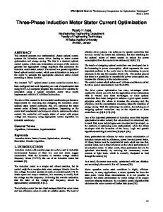
Although the LMC is cheap and faster, it is sensitive to the loss model inaccuracies, and parameters variation. In [12] G. Joksimovic´, A. Binder calculated the additional losses, at no load, in a high-speed squirrel cage induction motor fed from sinusoidal and inverter supplies. The additional no load losses in case of sinusoidal supply are due to the space harmonics and flux pulsations in rotor teeth. In case of using the inverter supply, there is increase in the losses due to the voltage harmonics. This harmonics produce additional high-frequency stator current components, which may cause firstorder skin effect losses in the parallel copper wires of the stator coils and secondorder skin effect in the conductors, (see Figure 1.6).

Figure 1.6: Measured iron losses and no-load additional losses at sinusoidal and inverter supply vs. fundamental stator frequency [12].

1. Introduction

8

The calculation of the motor losses for reference [12] was inserted in Appendix A.2. This model is accurate, but it needs information about the mechanical design of the motor, which is not usually available for all the motors. Figure 1.7 shows in general the block diagram of the loss model based controller for scalar and vector controlled induction motor.

f opt.

n ref

PI

−

2π

θe

∫

PWMVSI

v

Optimal loss model Eqs.

I.M

n (a)

n ref −

PI

i*q

v FOC

Optimal loss model Eqs.

i*d

PWMVSI

I.M

i

n

(b) Figure 1.7: Loss model a) in scalar control, b) in vector control.

1.2.3. Search control method In a search controller (SC), the motor input power is measured, and one physical quantity such as air gap flux or stator current or DC current is varied till the minimum input power is detected for a given load torque and speed [13-21]. The motor losses and their variation with reducing the flux for constant load torque and constant speed is shown in Figure 1.8. With reducing the flux from rated value, the motor copper loss increases, and the core loss decreases. The total loss decreases to a minimum value and then increases. The principle was first mentioned in [14]. He proposed to start the drive with a rated V/f ratio. When a constant torque demand is detected, the V/f ratio is reduced until the minimum DC link current is detected [15]. In [16] assumed that the machine operates initially at rated flux in steady state with low load torque at certain speed, as shown in Figure 1.8. The rotor flux is reduced in steps by reducing the flux forming current component ids, this results in an increase of the torque forming current component iqs. So, the developed torque remains constant. It is noticed that the core loss decreases with a decrease of the flux and the copper loss increases, but the total losses (motor and converter loss) decrease improving the overall efficiency. This is reflected in the decrease of the DC link power for the same output power. The search is continued until the system settles at the minimum DC link power (i.e., maximum efficiency) point A; any search attempt after point A adversely affects the efficiency and forces the search direction towards the point A.


9

Figure 1.8: Loss variation of Induction motor with flux decreasing for constant speed and constant load torque [16].

In [17], a minimization of stator current by search control instead of minimization of input power is derived. Figure 1.9 shows the use of the search control for scalar and vector controlled induction motor.

n ref

fs

PI

−

2π

θe

∫

V/f

PWMVSI

v − −

∫

every 50ms P

n P

n

−

Low pass Input power measurment filter

k

z-1

k-1

(a)

i*q

n ref

v

PI

−

i

∫ n

I.M

FOC

* d

− −

PWMVSI

I.M

every 50ms P

P

− k-1

k

Low pass filter

Input power measurment

z-1

(b) Figure 1.9: Search control a) in scalar control, b) in vector control.

The drawbacks of the search controller are:

1. Introduction

10

1) slow convergence and torque variations 2) extra hardware for measuring motor input power In [18], fuzzy logic controller was used instead of classic search control algorithm to make the algorithm convergence faster, as shown in Figure 1.10. n ref

i*q

PI

− Δn

fuzzy efficiency controller

Δn i*qs

Δi*d

PWMVSI

FOC

∑

i*d

I.M

n DClink power measurment

Pdc

n

n

v

Fuzzy Efficiency Controller

scaling factor computation

Pdc (k)

÷

ΔPdc (p.u.)

ΔPdc (k)

z −1

I b a se

P b a se

Fuzzy interference anddefuzzyfication

Δi*ds (p.u.)

Δ i*ds

ΔPdc (k − 1)

z −1 Figure 1.10: Search control using fuzzy logic controller.

In this model, the DC link power Pdc (k) is compared with the previous value to determine the decrement (or increment) ΔPdc (k) . Based on the input signals, the decrement step Δi dc (p.u) is generated from the fuzzy interface system. Instead of fuzzy logic controller, a neural network (NN) was used in the search control [22-24]. The NN structure is as shown in Figure 1.11. The model has one input layer, one hidden layer, and one output layer. The input layer includes two neurons to which the rotor speed and electromagnetic torque are connected as inputs to network. The output layer has only one neuron for the magnetizing current ids. A hybrid method is proposed in [25-27], using a LMC and SC where the first estimation is from the LMC and the subsequent adjustment of the flux is through the SC. ωr

i ds

T

input layer

hidden layer

output layer

Figure 1.11: Neural Network structure.

1.3 Formulation of the problem

1.3.

11

Formulation of the problem

Induction motors are large consumers of the electric energy, and many of them are not working all the time with their rated load torque. A significant improvement in the motor efficiency at partial loads can be achieved by using different control strategies. In industry, improving the efficiency for already working induction motors using search control method is not preferred for economic reason like requirement of the additional hardware. So, at first the thesis focuses on the efficiency improvement of squirrel cage induction motors fed by SVM-VSI using the loss model based method. A new expression for the optimal air gap flux is calculated from a detailed loss model. This loss model comprises the copper loss, iron loss, friction, windage, stray, and harmonic loss. The calculated optimal air gap flux is a function of these losses and also considers the non-linearity of the magnetizing inductance and the effect of the temperature on the motor parameters (stator and rotor resistances). Secondary, Measuring the efficiency of the induction motor according to IEEE-112B standard requires highly accurate measuring devices, where the inaccuracy of the power meter and torque meter should not exceed (0.1%), and (1 RPM) for speed sensor. But such devices are expensive. To reduce the measurement cost, an accurate system using a FPGA was designed to calculate the motor efficiency without requiring a power meter.

1.4.

Structure of the thesis

The thesis is divided into six chapters. Chapter two explains in detail the proposed loss model based controller and its implementation. The proposed loss model is used to improve the efficiency of a speed sensorless IFOC induction motor. The speed estimation, the stator and the rotor resistances estimation, and the motor stability are discussed. Also, it explains the proposed economic and accurate method to determine the motor efficiency. Chapter three presents the experimental set-up, the design of the accurate efficiency measurement system and comparison with an accurate power meter which has an accuracy of 0.1%. An economic inverter board was designed using an intelligent power module (IPM from Mitsubishi). Selection and design of the suitable DC link capacitor, current measurement sensor and heat sink are discussed in details. Chapter four clarifies experimentally the advantages of the proposed loss model in efficiency and power factor improvements. An on-line search control method is used to examine the accuracy of the calculated optimal flux values by the proposed loss model. Chapter five illustrates an improvement of a motor speed response, where the speed response can be improved by using a PI Fuzzy Logic speed controller instead of a conventional PI speed controller. Chapter six concludes the thesis.

12

2. The proposed loss model based controller and efficiency determination method

2.

The proposed loss model based controller and efficiency determination method

This chapter explains the proposed loss model based controller, and an accurate and economic measuring method for motor efficiency determination. In the proposed model, the motor electrical and mechanical losses are represented as function of the air gap flux. An on-line estimation for stator and rotor resistances is used to consider the effect of temperature and skin effect on winding resistances. Additionally, the non-linearity of the magnetizing current is included. This model uses an off-line calculated look-up table where the optimal flux values are stored for different motor load torques and different required speeds. The efficiency is determined from the calculated average electrical power and average mechanical power by FPGA. The electrical power is calculated by measuring and adapting two line-to-line voltages and two line currents instead of using power meter with accuracy equal 0.1% to fulfill IEEE 112B standard recommendation [29]. The average mechanical power is calculated from the measured load torque meter and speed sensor signals.

2.1.

Induction motor losses

The losses are classified as fundamental frequency losses and harmonic losses. The fundamental frequency losses consist of stator and rotor copper losses, core losses (eddy current and hysteresis), stray losses, and mechanical losses (friction and windage). The electrical losses are represented as shown in Figure 2.1 by the stator, the rotor, the stray, and core resistances.

R str

Rs

Xs

IS

V

Xr

E Ir

Im Xm

Rr/s

Rm

Figure 2.1: Single phase equivalent circuit for an induction motor.

2.1.1. Stator copper loss The stator copper loss is calculated as

Pcu,s =3I 2s R s where

2.1

Pcu,s

: stator copper loss

Rs

: stator resistance

Is

: stator current

2.1.2. Rotor copper loss The rotor copper loss is calculated as Pcu,r =3I 2r R r where

Pcu,r

: rotor copper loss

2.2

2.1 Induction motor losses

Rr

13

: rotor resistance

Ir : rotor current Temperature and influence of skin effect of the winding would be necessary for a correct copper losses calculation. To circumvent this, the stator and rotor resistances are estimated on-line by using adaptive motor parameter observer [28].

2.1.3. Core loss Energy lost by changing the magnetization of the steel laminations. Losses are due to eddy currents and hysteresis. From Steinmetz expressions for core losses, the hysteresis and eddy current losses in case of sinusoidal flux distribution are as follows. P h =k h φ 2 ωs 2.3

P e =k e φ 2 ωs2 2.4 where P h : hysteresis loss P e : eddy current loss k h : hysteresis coefficient given by material and design of the motor k e : eddy current coefficient given by material and design of the motor φ : flux linkage ω s : angular stator frequency So the stator core loss is

P s,c o re = k s,h φ 2 ω s + k s,e φ 2 ω

2 s

The rotor core loss is the same as stator core loss but with slip frequency instead of stator frequency. P r,core =k r,h φ 2 (sω s )+k r,e φ 2 (sω s ) 2 As the induction motor operates with a small slip, the rotor core loss is neglected compared to stator core loss. And the total core loss in the motor is 2.5 P core ≈ P s,core =(k h ω s +k e ω 2s ) φ 2 The equivalent per phase core loss resistance as shown in figure 2.1 is calculated as R m=

E2 P core

where E: induced back EMF

2.1.4. Friction and windage losses Energy lost in bearing friction and windage. Separation of friction and windage losses from core loss is made by reading voltage, current, and power input at rated voltage and rated frequency down to the point where further voltage reduction increases the current. It is represented as a function of the motor speed [8] as follows P fw = C fw ω 2 2.6 where Cfw is constant.

2.1.5. Stray loss The stray loss is that portion of the total losses not accounted for by the sum of stator copper loss, rotor copper loss, core loss, and friction and windage losses. One approximate representation of the stray loss assumes that the stray loss is proportional to the square of the rotor current and hence can be represented as additional resistance. It is represented by resistance (Rstr) in the stator branch, and is cal-

14


culated as follows [8, 31]. 2.7 P str = C str ω 2 I r 2 where Cstr is constant. According to IEEE 112B standard test procedure for induction motor, the stray loss is determined by measuring the total losses, and subtracting from these losses the sum of the friction and windage, core loss, stator loss, and rotor loss (indirect measurement).

2.1.6. Harmonic losses

1500 rpm 20

15 25

0.3

0.4

0.5

0.6

0.7

0.8

0.9

1

900 rpm 20

15

0.3

0.4

0.5 0.6 0.7 Load Torque (p.u)

0.8

0.9

1

as a percent of rated motor loss (%)

25

as a percent of rated motor loss (%)

Harmonic Loss (watt)

Harmonic loss (watt)

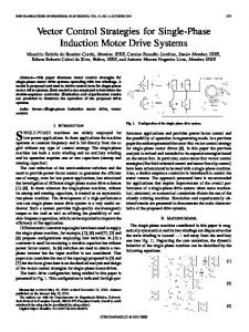
The harmonic losses are determined here experimentally for the tested 2.2 kW induction motor controlled by space-vector modulation. The total harmonic motor loss has been measured for different load torques and different speeds by using LMG 450 power meter as harmonic analyzer taken as the difference between the total motor input power and the fundamental component. As shown in Figure 2.2, the harmonic losses are about one percent (1%) of the motor rated power and five percent (5%) of the motor rated power loss, where the efficiency at rated load is 84%. So the harmonic losses are assumed equal 1% of the motor rated power ( Pr ). 2.8 P h ≈ 0.01Pr % 8 6 4 2 0 % 8 6 4 2 0

Figure 2.2: Harmonic losses for 2.2 kW Induction motor.

2.2.

Temperature and skin effect

Due to increasing the motor temperature both the stator and rotor resistances increase. The stator temperature can be measured, but it is difficult to measure the rotor temperature. The precise calculation of the temperature requires knowing of the thermal model of the motor. The skin effect in stator winding can be ignored, but it is prevailing in rotor bars of the squirrel cage. In an inverter fed machine, the skin effect due to the fundamental frequency can be ignored, but for the harmonic frequencies the rotor almost appears stationary, and therefore, practically all the stator harmonic currents flow in the rotor creating dominant skin effect [32]. An on-line estimation of the stator and rotor resistances is easier than measuring the temperature, and knowing the motor mechanical design data sheets. The estimation of stator and rotor resistances using the adaptive motor parameter observer will be explained in detail in section (2.5.3).

2.3 Non-linearity of the magnetizing current

2.3.

15

Non-linearity of the magnetizing current

The proposed model includes the non-linearity of the magnetizing current and the saturation effect. The magnetizing current is represented as function of air gap flux. I m = S 1φ + S 2 φ3 + S 3 φ5 2.9 where S 1 , S 2 , and S 3 are constants. These constants are calculated from the measured magnetizing current curve as shown in Figure 2.3. The motor parameters and constants are added in Appendix A.3. 0.7 0.6

Air gap flux (web)

0.5 0.4 0.3 0.2 0.1 0 0

0.5

1 1.5 2 Magnetizing current (A)

2.5

3

Figure 2.3: Magnetizing current curve.

2.4.

The proposed loss model

The motor losses are function in many variables such as stator current, rotor current, air gap flux, slip, speed, magnetizing current. Here, the total motor losses as function of air gap flux are represented by doing the required mathematical computations and suitable assumptions.

2.4.1. Induction motor variables From the motor equivalent circuit Figure 2.1, the following expressions are deduced. The induced back EMF and the magnetizing current expressions are E = ωs φ

Im = ωsφ / Xm

2.10 As the magnetizing reactance (Xm) is highly nonlinear, the magnetizing current is expressed as in Equation (2.9) I m = S 1 φ + S 2 φ3 + S 3 φ5 2.11 From equations (2.10) and (2.11) the magnetizing reactance is X m = ωs /(S 1 +S 2 φ2 + S 3 φ 4 ) 2.12 In addition, the rotor current is 2

Ir = E

⎛ Rr ⎞ 2 ⎜ ⎟ + ( Xr ) = ωsφ ⎝ s ⎠

2

⎛ Rr ⎞ 2 ⎜ ⎟ + ( Xr ) ⎝ s ⎠

The induction motor operates with a small slip, so tor current is approximated as

( Rr /s)

2

( Xr ) 2 holds and the ro-


16

Ir ≈ sωs φ R r The electromagnetic torque relation is R ⎛ 1− s ⎞ 2 Rr ⎛ 1− s ⎞ T = Ir 2 r ⎜ ⎟ = PIr ⎜ ⎟ ω⎝ s ⎠ ωe ⎝ s ⎠

2.13 2.14

where ωe : the electrical angular motor speed, and equal ( Pω ) P : pole pairs But the slip equation is

s= (ω s -ω e ) ω s

2.15

From equations (2.13), (2.14), and (2.15) we obtain sω s T = Pφ2 2.16 Rr The stator current is expressed as I s2 ≈ I 2r +I 2m 2.17 Combining equation (2.13) and equation (2.10) into equation (2.17), the stator current relation as function in air gap flux becomes 2

2

⎛ sω ⎞ ⎛ω ⎞ I ≈ ⎜ s ⎟ φ2 + ⎜ s ⎟ φ2 ⎝ Rr ⎠ ⎝ Xm ⎠ 2 s

2.18

2.4.2. Optimal air gap flux calculation The total power loss in the motor is Ploss = Pcu,s + Pcu,r + Pstr + Pcore + Pfw + Ph

=I 2s R s +I 2r R r +C str ω 2 I 2r +(k e ω 2s +k h ω s ) φ 2 +C fw ω 2 +P h

2.19

Combining equations (2.13), (2.18) into (2.19), the total power loss is 2 2 ⎛ ⎛ ⎛ sω ⎞2 ⎛ ω ⎞2 ⎞ ⎞ ⎛ sωs ⎞ ⎞ 2 ⎛ 2 2 ⎛ sωs ⎞ 2 2 s s ⎟ ⎟ ⎜ P loss =φ ⎜ RS ⎜ ⎜ + +R + φ C ω + K ω +K ω ⎟ ⎜ ⎟ ⎟ r⎜ ⎟ ⎜ ⎟ ( e s h s ) ⎟⎟ +Cfwω +P h str ⎜ ⎜ ⎜ R X ⎝ Rr ⎠ ⎠⎟ ⎝ Rr ⎠ ⎝ ⎠ ⎝ ⎝⎝ r ⎠ ⎝ m ⎠ ⎠ From equation (2.16) the flux is calculated as function of torque as φ2=

1 TR r P sω s

2.20

2.21

Therefore, the total power loss as function of torque is 2 ⎞ ⎛ Rs 1 1 Cstr ω2 ⎞ 1 TR r ⎛ ⎛ ωs ⎞ ⎜ Rs ⎜ Ploss = TRrsωs ⎜ 2 + + 2 ⎟+ + Keωs2 +Kh ωs ⎟ +Cfwω2 +Ph 2.22 ⎟ ⎟ P Rr Rr ⎠ P sωs ⎜ ⎝ Xm ⎠ ⎝ Rr ⎝ ⎠ Inserting the value of the magnetizing reactance -Equation (2.12) - into the previous equation gives 2 2⎞ ⎛ ⎛ TR r ⎞ ⎞ ⎟ ⎛ RS TR r 1 1 C str ω2 ⎞ 1 TR r ⎜ ⎛ Ploss = TR r sωs ⎜ 2 + + R S ⎜ S 1 +S2 +S3 ⎜ ⎟ ⎟ + ⎟+ P Rr R r2 ⎠ P sωs ⎜⎜ ⎜ sωs P sωs P ⎠ ⎟ ⎟⎟ ⎝ Rr ⎝ ⎠ ⎠ 2.23 ⎝ ⎝ 1 TR r + K e ωs2 +K h ωs ) +Cfw ω 2 +Ph ( P sωs 1 Assume X= (Inverse of slip speed) 2.24 sωs By using this assumption - Equation (2.24) - in equation (2.23), the total power loss as function of (X) is

(

)

2.4 The proposed loss model

TR r Ploss = PX

17

⎛ RS 1 C str ω 2 + + ⎜ 2 R r2 ⎝ Rr Rr

2 2 ⎞ ⎛ ⎞ ⎞ TR r X ⎛ TR X TR X ⎛ ⎞ r r ⎜ R S ⎜ S1 +S 2 +S3 ⎜ ⎟⎟ ⎟ + ⎟+ ⎟ ⎜ P ⎜ P P ⎝ ⎠ ⎠ ⎝ ⎠ ⎠⎟ ⎝

2.25

TR r X ⎛ ⎛1 ⎞ ⎛1 ⎞⎞ 2 ⎜⎜ K e ⎜ +ω e ⎟ +K h ⎜ +ω e ⎟ ⎟⎟ +C fw ω +Ph P ⎝ X X ⎝ ⎠ ⎝ ⎠⎠ 2

+

For simplicity assume these abbreviations: ⎛R TR r 1 C ω2 ⎞ C1 = , C2 = ⎜ S2 + + str 2 ⎟ P Rr ⎠ ⎝ Rr Rr Using them in equation (2.25) gives 2 ⎛ ⎛1 C1C2 2 2⎞ ⎞ ⎛1 ⎞⎞ ⎛ Ploss = +C1X ⎜ R S S1 +S2 C1X+S3 ( C1X) ⎟ +C1X ⎜ Ke ⎜ +ωe ⎟ +Kh ⎜ +ωe ⎟ ⎟ +Cfwω2 +P h 2.26 ⎜ X ⎝ ⎠ ⎠ ⎝X ⎠ ⎟⎠ ⎝ ⎝X The loss minimization with respected to the flux at steady state is calculated according the following condition d P lo s s 2.27 T ,ω = 0 dφ Representing the torque in equation (2.16) as function of (X) gives

(

T=

)

P 2 1 φ Rr X

2.28

If we have a speed controller and the flux changes by Δφ ≠ 0 and a constant load is applied, then the speed controller will produce the same torque ( ΔT = 0 ) in steady state. ΔT 0 = =0 Δφ Δφ

The derivation of equation (2.28) with respect to φ is ΔT P 1 1 dX = (2φ -φ2 2 )=0 Δφ R r X X dφ 1 1 dX ∴ 2φ =φ2 2 X X dφ

∴ dφ =

φ dX 2X

2.29

Inserting equation (2.29) into (2.27) gives dP loss dP loss 2X = =0 dφ dX φ So the new criterion for getting minimum power loss is given as follows dP loss =0 dX

2.30

The derivation of equation (2.26) with respected to (X) gives a sixth order polynomial function in (X) as follows (the derivation is shown thoroughly in appendix A.4)

α 0 +α1X+α 2 X 2 +........+α 6 X 6 = 0

2.31 The coefficients of this equation are functions of the motor parameters, motor speed, and the electromagnetic torque (which will be estimated). By solving equation (2.31) the optimal value (Xoptimal) is calculated. By using equation (2.28), the optimal flux ( φoptim al ) is calculated as φoptimal =

T R

r

Xoptimal P

2.32


18

Figure 2.4 shows the calculated optimal air gap flux for different load torques and different speeds to improve the efficiency of the tested 2.2 kW squirrel cage induction motor.

Optimal Flux (p.u)

1 0 .9 0 .8 0 .7 0 .6 0 .5 1 1500 1200

0 .5

900

L o a d T o rq ue (p .u)

0

600 300

S p e e d (rp m )

Figure 2.4: The optimal air gap flux for different load torques and different speeds.

2.5.

Implementation of the proposed loss model

The implementation comes through two steps. 1) By solving equation (2.31) for different values of torque and speed and storing the values of optimal flux versus torque and speed in a look up table (Off-line). Matlab was used for the calculations. 2) While running the motor, the torque is estimated by an observer and from the look up table the optimal flux is read (on-line). A PC was used for the on-line control. Figure 2.5 shows the block diagram of the optimal air gap flux calculation from the estimated torque.

T Estimated torque

n

X optimal LU T

φ optimal

Estimated speed

Rr Rotor resistance

1 P

Optimal flux

Figure 2.5: Block diagram of the optimal air gap flux calculation.

The proposed loss model can be used in drives with scalar control as well as in drives with vector control. In vector control the rotor speed is measured using a speed sensor or calculated based on the electrical motor quantities (speed-sensorless). The interest in speed sensorless control emerged from practical application where high control quality is required but the speed sensor is either difficult to use due to technical reasons, or too expensive. So, using the proposed loss model to improve the efficiency of speed sensorless indirect field oriented controlled induction motor is suggested in this thesis. The block diagram is as shown in Figure 2.6.

2.5 Implementation of the proposed loss model

19 Diode Rectifier

− n

i *ds

vd

2

PI ∗

÷

i *qs

T

d, q

PI

−

2 2 Lr 3 P L2 m

vq

PI

−

vα

va vb vc

vβ

α,β

i ds

αβ ,

iα d, q

i qs

n

a,b,c

α,β

βk

IFOC

iβ

ia ,ib ,ic a,b,c α, β

S p ee d e stim atio n ∧

RS ∧

Rr

3 P L2 m 2 2 Lr

T

1 Lm

L UT

Xopt.

parameters estimation observer

1 P

Field Oriented Control

nref

1

Speed Parameter Estimation Estimation

i dsr i ds ( opt .)

I.M

Inverter

φopt.

Loss Model Controller

A C supply

Hardware

DC Link

Figure 2.6: The optimal flux loss model based on speed sensorless vector control induction motor block diagram.

The block diagram consists of four blocks. FOC, speed estimation, parameters estimation observer, and proposed loss model block diagrams. The following sections explain each block separately.

2.5.1. FOC block diagram In general, the field-oriented control can control the rotor flux linkage and the torque independently. Values of the flux producing current component i *ds and the torque producing current component i *q s are given. Each of these two components is controlled by a PI controller. The controller output is the voltage vector in dq-reference frame, which transformed into αβ -reference frame by a vector rotator. Then, the switching times are calculated and the inverter impresses the voltage vector on the motor. Another vector rotator transforms the measured currents into the dq- reference frame. The resulting components are sent to the current controllers. The angular position of the rotor flux linkage βk , which is required by the vector rotators, is calculated by indirect means (IFOC) [33], from the measured currents and the estimated rotor speed. The field-oriented control is primarily a current control. It is used together with a higher-level speed control. The speed controller calculates the torque producing current component as a function of the speed, which evaluated by the current controller. So, the controller is a cascade control structure. That means that the outer control

20


loop is speed controller controls the speed, its output is the reference torque. The inner controller is the current control loop, which controls the current to its reference values that is calculated from the reference torque value.

2.5.1.1. PI current controller The current control loop of d-axis is working as follows. In the transient, such as at the beginning of the operation (motor starting) and in case of load changing, the reference flux-forming current component i *d s is established to the rated value idsr (=2.9A). In steady-state, the reference current i *d s is reduced to the optimal value

i ds(opt.) that is generated from the loss model controller. The loss model controller becomes effective only at steady-state condition. That is, when the speed error approaches zero. The simplified current control loop of q-axis is as shown in Figure 2.7, where the coupling inductances between the d-q axes are neglected. The control’s time delay (included inverter reaction time) is represented by a first order lag element with a time constant TD = 1.5Ts where Ts is the sampling time [34]. The converter gain kc is the relation between the numerical evaluation in the computer (digital controller) and the real output voltage. In this case the resolution scale used was 4000 (12 bits) for the complete line to line voltage (2/3 DC-Link voltage), which is calculated as follows 2/3U dc kc = , 4000 for Udc=600 V, so kc=0.1. The electrical gain k elec and the electrical time constant Telec of the motor are respectively kelec = 1/ Rs Telec = ls / Rs The PI controller setting according to the amplitude optimum criteria and its transfer function is represented as follows [34] G R ( s ) =K p

1+sTi sTi

The coefficients k p and Ti are calculated as follows

ls 2k c TD Ti = Telec Kp =

E(s)

I*q (s)

Iq (s)

e(s)

Kp

1+Ti s Ti s

U*q (s)

kc TDs+1

Uq (s)

D elay

PI C o n tro lle r

C o n tro l tim e d elay

Figure 2.7: Simplified PI current controller.

k elec Telec s+1 Plant


21

2.5.2. Speed estimation Field oriented control method is widely used for the induction motor drives. For high precision and high dynamic, a speed sensor is necessary for speed signal feed back. However, a speed encoder cannot be mounted in some cases. Such as motor drives in a hostile environment, high speed motor drives. Also, a speed encoder is undesirable in a drive because it adds cost, reliability problems, and the need for a shaft extension and mounting arrangement. These entire problems are solved by using the sensorless vector control methods. Sensorless vector control of the induction motor is presented in [35-40]. The speed is estimated by measuring the motor terminal voltages and currents. The speed can be estimated by one of the following methods: - slip calculation. - direct synthesis from state equation (motor back EMF equations). - model referencing adaptive system. - speed adaptive flux observer. - extend kalman filter. - slot harmonics. - injection of auxiliary signal on salient rotor. The aim is to improve the efficiency of the sensorless controlled induction motor by the suggested loss model, and not to investigate a new method or develop one of the known speed estimation methods. So, here the speed is estimated from motor back EMF equations [56], which is easy to implement but its disadvantage that it does not work at standstill. From the equivalent circuit of the induction motor in the stationary reference frame ( α, β ) [16], as shown in Figure 2.8, rotor voltage equations are as follows

i αs

i αr L ls = L s − L m

Rs

Vαs

φα s

L lr = L r − L m

Lm

Vβs

ωr φβr

φα r

iβs Rs

Rr

iβr L ls = L s − L m

φβ s

L lr = L r − L m

Lm

Rr

φβ r

Figure 2.8: α − β Equivalent circuits in stationary reference frame.

ωr φαr

22


R r i αr + ρ φ αr + ω r φβ r = 0 R r iβ r + ρ φβ r − ω r φ αr = 0

2.33

where ρ = d /d t The rotor currents are 1 iαr = ( φ α r -L m i α s ) Lr

2.34 1 iβr = ( φβ r -L m i β s ) Lr Resolving equation (2.33) and using (2.34), the estimated speeds are R R L ω r = (ρ φ β r + r φ β r − r m i β s ) / φ α r = A / φ α r 2.35 Lr Lr R R L ω r = ( −ρφ α r − r φ α r + r m i α s ) / φ β r = B / φ β r 2.36 Lr Lr While the rotor flux components are calculated from the stator flux and stator current components as follows L φ α r = r ( φ αs − σ L s i α s ) Lm L φβ r = r ( φ β s − σ L s i β s ) Lm and σ = (Ls Lr − Lm ) / Lr Ls (Blondel’s leakage factor) The stator flux components are estimated by integrating the stator back- EMF using a low pass filter. 2

1 (Vα s − R s i α s ) s+a 1 = (Vβ s − R s i β s ) s+a

φ αs = φβs

Where (a) is the cut-off frequency (a=3 Hz), (s) is Laplace Operator. The numerator of equation (2.35) depends on the current component i β s , and the numerator of equation (2.36) depends on the current component i α s , but the accurate calculation of each component differs from the other due to a difference of the accuracy in measuring the three motor currents. So, it is better and more accurate to include the two current components i α s and i β s in one equation as follows Equation (2.35) can be rewritten as

A A ωr = = φ αr φ αr

φ α2r +φ β2r φ α2r +φ β2r

or

ωr =

A2 2 A2 2 φ αr + 2 φ βr φ αr2 φ αr φ αr2 + φ βr2

From equations (2.35), and (2.36)

2.37


23

A B = φ αr φ β r By inserting equation (2.38) in (2.37) the estimated speed is

ωr = ωr =

2.38

A 2 2 B2 2 φ αr + 2 φ βr φ α2r φ βr φ α2r +φ β2r A 2 + B2 φ α2r + φ β2r

The block diagram of speed estimation is as shown in Figure 2.9.

Iαs σ Ls

Rs

Vαs

φαs

∫

Lr Lm

Rr Lr

Rr Lm Lr

B X

a

-

X

d dt

÷

a

Vβs

φαr

-

X

∫

φβ s σ Ls

Rs

Lr Lm

φβ r

Rr Lr

ωr

A X

d dt

Iβs

−

Rr Lm Lr

Figure 2.9: Speed estimation block diagram.

The indirect field oriented control of an induction motor is sensitive to motor parameters variation. Especially, rotor and stator resistances vary with the motor temperature. Additionally, the proposed loss model controller depends on the motor parameters. Therefore, an on-line estimation of the motor parameters is necessary for the IFOC and for the proposed loss model. The following section explains the estimation of the stator and rotor resistances by using the parameter adaptive observer [28].

2.5.3. Parameters estimation A standard smooth air gap model for the induction motor can be described by a state equation in stator reference frame as following. d 2.39 x = Ax + Bu dt y = Cx 2.40 T

where u= ⎡⎣ vαs vβs ⎤⎦ : stator voltage vector T

x= ⎡⎣i αs iβs φαr φβr ⎤⎦ : motor states

24


y= ⎡⎣iαs iβs ⎤⎦

T

: stator current components

A12 ⎤ ⎡ A11 T T , B = [ B1 B2 ] , C = [ C1 C2 ] A=⎢ ⎥ A 22 ⎦ ⎣ A 21 and A11 = − {R s /(σLs ) + (1 − σ) /(στ r )} I = a r11I A12 = L m /(σLs L r ) {1/(τr )I − ωr J} = a r12 I + a i12 J

A 21 = (L m / τr )I = a r 21I A 22 = −(1/ τr )I + ωr J = a r 22 I + a i22 J B1 = 1/(σLs )I = b1I , σ = (1 − L2m / L r Ls ) ⎡1 0 ⎤ I=⎢ ⎥ ⎣0 1⎦ ⎡0 − 1⎤ J=⎢ ⎥ ⎣ −1 0 ⎦ C1 = I 0⎤ ⎡0 B2 = C 2 = ⎢ 0 ⎥⎦ ⎣0 Figure 2.10 shows Luenberger observer which estimates the stator current and the rotor flux in stator reference frame by the following equations. dx = Ax + Bu + G(y − y) = A L x + BL u L 2.41 dt y = Cx 2.42 where A L = A + GC , BL = [ B − G] , u L = [ u y] T x = ⎡⎣ iαs iβs φαr φβr ⎤⎦ : the estimated states of the motor u = ⎡⎣ v α s v β s ⎤⎦

B

T

y = ⎡⎣ i α s i β s ⎤⎦

Induction M otor

dx dt

∫

x = ⎡⎣ iαs

A

iβs

φαr

T φβr ⎤⎦

A daptive schem e

R s , τr

C

T

⎡ iαs ⎣

T iβ s ⎤⎦

y = ⎡⎣ iαs

i ⎤ T βs ⎦

y=

G Figure 2.10: Block diagram of parameter adaptive observer.


y = ⎡⎣ iαs

25

T iβs ⎤⎦ : the estimated output of the observer T

g2 g3 g 4 ⎤ ⎡ g1 G=⎢ ⎥ : the observer gain matrix g g g g − − 1 4 3⎦ ⎣ 2 Coefficients of the observer gain matrix G are chosen so that the Luenberger observer can be stable. The most frequently used method is based on the fact that the observer eigenvalues are chosen in such a way that they are proportional to the motor eigenvalues [41]. The induction motor itself is stable, so the observer is also stable in usual operation. Coefficients of G matrix are

g1 = (k − 1)(a r11 + a r22 )

g 2 = (k − 1)a i22 g 3 = (k 2 − 1)(ca r11 + a r 21 ) − c(k − 1)(a r11 + a r 22 )

g 4 = −c(k − 1)a i22 , c = (σLs L r ) / L m Figure 2.11 shows the eigenvalues for different values for (k) by solving the following equation. A L − λI = 0 , ( λ ) is eigenvalues For k = 0, 0.2, 0.6,1, and 1.1 all roots are negative and the observer is stable, but for k=1.2 and 1.5 the roots are positive and negative (observer is not stable). In Figure 2.10 the induction motor (equation 2.39 and 2.40) represents the reference model, while Luenberger observer (equation 2.41 and 2.42) is considered as adjustable model where it includes unknown parameters. From the error between the reference model and adjustable model, the stator resistance and the rotor time constant are calculated from the following adaptive scheme. The difference between the estimated output and the real (measured) one is

y=y-y , x=x-x

Imag.

1

* * * *

0.8 0.6 0.4 0.2

k=0 k=0.2 k=0.6 k=1.0 k=1.1 k=1.2 k=1.5

Real

0 -0.2 -0.4 -0.6 -0.8 -1 -4000

-3500

-3000

-2500

-2000

-1500

-1000

-500

0

500

Figure 2.11: Eigenvalues for different values for k.

dx dx dx = (A+GC)x+Ax , = dt dt dt

2.43

11 ⎡A A=A-A= and ⎢ ⎣ A 21

2.44

12 ⎤ A 22 ⎥⎦ A

26


where 11 =- { R s /(σLs )+ (1-σ)/(στ r ) } I A

12 =Lm /(σLs L r )1/(τ r )I A 21 =(L m /τ r )I A

22 =(-1/τ r )I A The following Lyapunov function is defined as a candidate for simultaneous stator resistance and rotor time constant [41] estimation.

V=x T x+

R 2s L + m2 λ1σL s λ 2 στ r

λ1 and λ 2 are positive constants. By deriving the Lyapunov function and using (2.43) and (2.44), it gives dV T 2R s dR s 2R s =x ⎡⎣ ( A+GC )T + ( A+GC ) ⎤⎦ x+ ( i i +i i ) dt λ1σLs dt σLs αs αs βs βs 2L m d 1 2L m i φ +i φ ) - 2 ( 1-σ ) ( i i +i i ) + + ( αs αr βs βr αs αs βs βs λ 2 στ r dt τ r σLs L r τ r στ r dV For stability criteria of Lyapunov, must be negative. The first dt x T ⎡⎣ ( A+GC )T + ( A+GC ) ⎤⎦ x is always negative because of the imposed eigenvalues of the observer. So the other terms can be set to zero or value less than zero. Here the other terms are divided to two terms each of them equal zero as follows

2R s dR s 2R s ( i i +i i ) = 0 λ1σLs dt σLs αs αs βs βs 2L m d 1 2L m i φ +i φ ) - 2 ( 1-σ ) ( i i +i i ) = 0 + ( αs αr βs βr αs αs βs βs λ 2 στ r dt τ r σLs L r τ r στ r

2.45 2.46

Equations (2.45) and (2.46) can be rewritten to express the changing in the stator current and the rotor time constant like

dR s =λ1 ( iαs iαs +iβs iβs ) dt λ ( 1-σ ) d 1 λ =- 2 ( iαs φαr + iβs φβr ) + 2 ( iαs iαs +iβs iβs dt τ r L s L r Lm λ λ L = - 2 ( iαs φαr +iβs φβr ) + 2 m ( iαs iαs +iβs iβs ) Ls L r Ls L r λ = - 2 ( iαs ( φαr − L m iαs ) + iβs ( φβr -L m iβs ) ) Ls L r

)

Figure 2.12 shows the simulated and experiment results of the parameters estimation. The Initial value of the estimated stator resistance is 1.3 time as much as actual value, and the initial value of the estimated rotor resistance is 1.4 time as much as actual value. The constants λ1 , λ 2 , and k are 0.05, 0.2 , and 1 respectively. As for k=1, gain matrix G is zero and the motor model is simple and stable.

3 2.5

130% actual value

2 1.5

actual value=1.6Ω

1 0.5 2

4

6

Time (s) (sec) Time

3

130% actual value

2.5 2 1.5

actual value=1.6Ω

1 0.5 0 0

1

2

3 4 Time (s) (sec) Time

5

3.5

140% actual value 3

6

actual value=2.2Ω

2.5

Estimated Rotor Resistance (ohm)

Estimated Rotor Resistance (ohm)

Estimated Resistance (ohm) Estimated Stator Stator Resistance (ohm)

0 0

27 Estimated EstimatedRotor RotorResistance Resistance(ohm) (ohm)

Estimated Stator Resistance (ohm)


2 0

2

4 Time (sec) Time (s)

6

3.5

140% actual value 3

2.5

actual value=2.2Ω

2

1

2

3

4

Time (sec) Time (s)

5

6

Figure 2.12: Estimated stator and rotor resistances.

2.5.4. Motor stability If there is a load increase while the motor is operated with the optimal flux value,

iids*(A) ds (A)

4 2

*

0

5

10

15

Motor Input Power (watt)

1500

20

25

30

w ith o p tim a l f lu x

w ith ra te d f lu x

1170 1115

a t n o lo a d w ith w ith ra te d f lu x o p tim a l f lu x

500

a t 5 0 % r a t e d lo a d

300 180

Load Torque (N.m) Speed(rpm) Load Torque Speed(rpm) (Nm)

50 5

10

15

20

25

30

5

10

15

20

25

30

5

10

15

20

25

30

1500

0 10 5 0

0

TTime ime(s)(sec)

Figure 2.13: Measured flux producing current component, motor input power, speed, and load torque with rated and optimal flux at load changing from no load to 50%.

28


* the reference flux producing current component i ds will be increased to the rated

value i d sr , and after this, the suitable optimal flux value according to the new load torque is calculated. *

In Figure 2.13 the reference flux producing current component i d s is reduced from the rated value

i dsr

to the optimal one

i ds(opt ) while the motor running at no load, the

absorbed motor input power is reduced by 40%. Then the motor is loaded with 50% of the rated load, so the current is increased to the rated value to face the sudden increase in the load torque, after that it is reduced to the new optimal value, and the improvement in the efficiency is 4.5%. Another test was done by increasing the load torque from no load to 65% of the rated torque while the motor operates with the optimal flux. As shown in Figure 2.14, *

i ds

*

(A)

the reference value of the i d s directly is increased to the rated value to face the sudden increase in the load torque, after that it is reduced to the new optimal value, and the improvement in the efficiency is 2.3%. In case of increasing the load torque to 65% of the rated value, the reduction in speed is more compared with increasing the load torque to 50% of the rated torque, because the load torque is higher. During the step load changing, the speed reduces from the reference value but in less than one second returns to the its reference value.

*

3 2 1

ra te d

o p tim a l

ra te d

o p tim a l

0 .6 5 p .u L oad

no L oad

1 7 00

Motor input power (watt)

1 5 70 1 5 30

1 0 00

3 0 0 1 8 0 1 0 0

Load Torque(N.m) Load Torque (Nm )

(rpm) SSpeed p eed (rpm )

1500 1000 500

15 10 5 0

5

T Time i m e(s)( s e c )

10

15

Figure 2.14: Measured flux producing current component, motor input power, speed, and load torque with rated and optimal flux at load changing from no load to 65%.

2.6 Determination of the efficiency

2.6.

29

Determination of the efficiency

According to IEEE 112B standard test procedure for polyphase induction motors and generators [29], efficiency is the ratio of output power to total input power. Output power is equal to input power minus the losses. Therefore, if two of the three variables (input power, output power, or losses) are known, the efficiency can be determined by one the following equations. output power Efficiency= input power input power-losses Efficiency= input power output power Efficiency= output power + losses In [29] ten methods of efficiency and losses determination are identified, from which method B, Input-output with segregation of losses and indirect measurement of stray load losses is chosen here for the measurement. This method should be selected when the value for each of the components of the losses in the motor is of interest (i.e. in the proposed loss model) or when the precision is required. As the proposed loss model depends on the calculation various loss components, method B is the suitable one for efficiency and loss determination. In method B the motor input power, the mechanical load torque, and the motor speed should be measured with accurate measuring devices. The accuracy of the used power meter and torque meter should be better than 0.1% and 1 RPM for speed sensor. Using method B in measuring efficiency of motors, the electrical input power at the 3-phase, 3-wire ac terminals together with the mechanical output power has to be measured. The measurement of the mechanical output power has to be done by measuring the shaft torque by a precision torque transducer between the tested motor and the load machine and simultaneous measurement of speed. The measurement equipment is expensive. In this thesis, a cheap and accurate system is designed to determine the motor efficiency without requirement of power meter by calculating the average electrical input power by measuring two line-to-line voltages and two line currents as follows.

2.6.1. The proposed measuring method Firstly, the real electrical power is defined as the time-average of the instantaneous power. According to Figure 2.15, the instantaneu1M (t) ous power is i1 (t) 1 p(t)=u1M(t)*i1(t)+ u2M(t)*i2(t)+ u3M(t)*i3(t). Substituting i2(t)= -i3(t)-i1(t) gives, p(t)=(u1M(t)-u2M(t))*i1(t)+ (u3M(t)-u2M(t))*i3(t) p(t)=u12(t)*i1(t)+ u32(t)*i3(t) Two currents and two phase-to-phase u 2M (t) i2 (t) voltages have to be measured; this is the M well-known “2-Watt Meter” approach by 2 Mr.Aron. The designed system consists of two boards (will be explained in detail in chapter u3M (t) 3); the first one adapts the input analog signals (motor voltages and currents signals, 3 i3 (t) load torque meter signal, and position enFigure 2.15: 3-Phase, 3-wire. coder signals), so it is called Analog Signal

30


I2.2

I1.2

I2.1

I1.1

Conditioning board (ASC). The U1-2 .1 U3-2 .1 U1-2 .2 U3-2 .2 ASC board translates 4 higher voltage and 4 current signals to low voltage signals (600VÆ0.5V and 15AÆ0.5V) suitable for A/D converters. Additionally, a torque AD8131 meter signal (50NmÆ0.5V) is Differential LF 356N Amplifier Op. Amp used. The bandwidth of the signal ±5V conditioning is 100 kHz, (See Fig±15V T.in ure 2.16). The second board includes the Figure 2.16: Analog Signal Conditioning board. A/D converters and the FPGA. In this board the adapted analog signals is converted to digital, so it is called Sensor to Digital board. Figure 2.17 shows the Sensor to Digital PCB. There are up to 5 sets of Analog inputs, each set consists of two Analog signals (ca. 1Vpp). The signals of one set are simultaneously converted by two 12-bit A/D-Converters (conversion time ca. 1µs). There are two sets of two A/D-converters (set A and set B). Both can work simultaneously. Set A is connected via multiplexes to the odd input connectors with the signals In1.1, In1.2, Figure 2.17: Sensor to Digital board. In3.1, In3.2, In5.1, and In5.2. Set B is connected via multiplexes to the even input connectors with the signals In2.1, In2.2, In4.1, and In4.2.

2.6.2. The proposed sampling for efficiency determination

Conversion start

Conversion start

Conversion start

Conversion start

Conversion start

Conversion start

A C- M achine +Torque shaft +Encoder

To determine the efficiency, two inputs for the two voltage A/D-Conv. Input Signal Input Signal Input Signal In1.1=Enc Sin A1 In5.1=Torque signals, two inputs for the curIn1.1=Enc Sin In1.2=Enc Cos In5.2=NC A2 In1.2=Enc Cos rent signals, one for the load ca.2µs ca.2µs ca.2µs torque meter signal, and two for the position encoder signals (Sin and Cos signals) are used. Figure 2.18 shows the proA/D-Conv. Input Signal Input Signal Input Signal posed sampling for efficiency In2.1=u12 B1 In4.1=i1 In2.1=u12 In2.2=u32 In4.2=i3 In2.2=u32 B2 determination of an ACi1 ca.2µs ca.2µs ca.2µs machine. In the first sampling Torque AC-Machine interval all the torque-signal +Torque shaft EncSin +Encoder and the Sin and Cos-signal i3 EncCos from the encoder are sampled and converted. In the next Figure 2.18: Sampling for efficiency determination. sampling interval signals defining the input power are sampled and converted simultaneously.

2.6.3. Electrical and mechanical powers calculation Figure 2.19 illustrates the calculation of the 3-phase electrical power, e.g. at the terminals of an AC-machine. First, there is a correction of offset and gain for each channel. The correcting values were determined by a calibration procedure prior to

2.6 Determination of the efficiency

31

Offset i Gain i the measurement. The power values i + 1 + are accumulated and finally divided by the number of processed samples. average The calculation of the mechanical V 1-2 electrical power is as shown in Figure 2.20. The input + + power + primary sampling intervals ∆ts=4µs are G ain V Offset V accumulated much too short to calculate the speed. power Offset i 3 Gain i 3 + + The speed-error would be very high. samples i3 + + We assume nearly constant values of number z-1 speed and torque for time intervals ∆tc=100µs. This is justified by the fact, V 3-2 that frequency of torque ripple corre+ + Offset V sponds to the switching frequency or G ain V the inverter, which is 1/200µs=5 kHz. Figure 2.19: Calculation of the average The position calculation is (in Figure electrical input power in the FPGA. 2.20) detecting and counting the zerocrossings of Sin and Cos signals using each primary sample. Finally, the change of position within the last 100µs (=25 samples) is calculated using fine interpolation with arctan. The torque is accumulated for the same ∆tc=100µs interval. After dividing the change of position by the average torque in the last ∆tc=100µs interval, we get the average speed and the average torque in the last ∆tc=100µs interval. From this the average mechanical power is calculated as shown in Figure 2.20. 1

1-2

3-2

Offset Gain Torque

Arc Tan

Counter

Zero crossing

E nc C os

1 -2

3 -2

Average speed in the last 100µs

Position calculation

E nc S in

1

Change of Position Within the last Δ tc= 100µs interval Δ tc= 100µs Samples=25

Average power in the last 100µs

+ +

Calculation once each 4µs interval

Accumulated Power z-1

Accumulated Torque z-1

+

Avarage Power

Δ tc= 100µs Samples=25

Average torque in the last 100µs

Number of accumulated Δ tc interval

Calculation once each 100µs interval

Figure 2.20: Calculation of average mechanical output power in the FPGA.

32

3.

3. Experimental set-up

Experimental set-up

The designed set-up to control the induction motor as variable speed dive (VSD) and the efficiency determination contains two main parts. First part describes the so called inverter board which includes the inverter module, DC link capacitors, diode bridge rectifier, current sensors, optocouplers and heat sink, while the inverter interface board is already designed in previous work [42]. The second part describes the designed efficiency determination system, which consists of the Analog signal conditioning (ASC) board and sensor to digital (S2D) board. The hardware of the S2D board was also designed in a previous work [57] The scheme of the experimental set-up is as shown in Figure 3.3.

3.1.

The motor

Table II shows the parameters of the tested 2.2kW induction motor. Parameters are calculated from the motor’s manual , the no load and blocked rotor testes. Table II. Ratings of the tested 2.2kw Induction Motor Rated voltage 360V Stator inductance 17mH Rated current 6A Rotor inductance 17mH Stator resistance Rotor resistance frequency

1.6Ω

Rated speed

2.1Ω

Moment of inertia

50 Hz

Insulation class

1420 rpm 0.00479 kgm2 F

HANNING industrial motor (2.2 kW)

3.1.1. Coupling and load The tested motor is loaded by 3.1KW DC machine as generator. The armature winding of the DC generator is connected in parallel with a variable resistor as a variable load. The two motors are coupled by RADEX-NC steel disc coupling, and in between a torque measuring shaft DATAFLEX 22/50 is inserted as shown in Figure 3.1 [43]. The maximum measured torque using the torque meter is 50Nm. The analog output value of the torque is available as voltage signal with ratio 1V/10Nm and current signal with ratio 1.6mA/10Nm. The Figure 3.1: The torque meter and couvoltage signal was used for the measurement. pling. The required supply voltP age for the device is 24V U IPM 1200 V V DC with a maximum curPS22056 Snubber W To Motor capacitor terminals rent consumption of N 100mA. EVBPS 22056 The advantage of the 6X PWM 1X FO DC- link device is that all the elecCapacitor tronics are located in the + 15 V +5 V fixed housing so that no Interface Board additional equipment is Diode Rectifier needed to send the signal, 400V ∼ and its accuracy is 0.2%.

3.2.

Inverter board

Figure 3.2: IPM evaluation board and the required external hardware.

3.2 Inverter board

33

With the progress in inverter technology, using the intelligent power module (IPM) which is hybrid power devices that combine IGBTs with gate drive and protection circuits all built inside the same module is better than isolated discrete power devices with additional drive and protection circuits.

P C I-In te r fa c e

R S 4 8 5 - 1 6 b it p a r a lle l

P C I-In te r fa c e

PC

S e n s o r to D ig ita l (S 2 D )

Drive Module Interface

Torque

A n a lo g S ig n a l C o n d it i o n i n g (A S C ) U 1 2 U 3 2C o s S in

7 Optocouplers F0

+ 1 5 -1 5 M

IGBT-Drivers

LE M

+ 1 5 -1 5 M

IPM

N

PS22056

+1 5 -1 5 M

K31L3

220Vdc

0,8 A max.

A A F1

Hanning Typ193/ 4FBT-091 208/360V, 6A 2,2kW, 1420U/min

F2 A1

B1

DC-Load Machine

Toruqe measuring shaft

Induction Machine DUT

IncrementalEncoder

GM 32: 230V dc, 1500U/min 13 A dc ; 3,1kW

Couplings

F2

K0 Main Switch Hauptschalter

L1 L2 L3 PEN

(Automat 16A)

X1

K2 Lampe rot, Front Hauptschalter = Ein

K1h

HilfsSchalter

F1 (Neozed 16A)

Steckdose mit Filter 3-fach (PC+...)

(Schütz Contactor)

H0

PE

K1

Lampe gelb, Oben Schütz = Ein

L1 L2 L3

1L3 H1 n E2 p

NF 2

1L3

1 ph Netzfilter

1L3

R S 4 8 5 - 1 6 b it p a r a lle l

K1

T2 (Ein On) T1 (Aus Off)

K1

N

Figure 3.3: Experimental set-up scheme.

N

25A

200Ω 30A 25A

N

34

3. Experimental set-up current signals

current sensors

DC link Capacitors

U U1

conector

±15V,±5V

Interface board

V

control signals

V1 W V

W W1

U

P

N P

a

Optocoupler

400V AC Supply

c

6X PWM 1X FO

N

15V,5V conector

N b bridge diode rectifier

IPM evaluation board Heat sink Figure 3.4: The designed Inverter Board.

IPM provides a complete solution by integrating all these discrete components in a transfer molded package. It does not only simplify the system configuration and reduce the system space and parts number, but also achieves an improved reliability and flexibility. Mitsubishi developed an evaluation board [44] which consists of the IPM module, bootstrap circuit and snubber capacitor. In this thesis the IPM evaluation board (EVBPS22056) was used. But there is external hardware required for controlling the motor as variable speed drive as shown in Figure 3.2. As shown in Figure 3.4, a board was designed including the required external hardware such as the DC link capacitors, current measurement sensors for control purpose, and optocouplers for isolation. The diode bridge rectifier and the IPM are supported on suitable heat sink. In the following sections the calculation and choosing the suitable values for the external hardware are explained in detail.

3.2.1. IPM evaluation board The main element in the evaluation board (Mitsubishi order no. EVBPS22056) shown by green color in Figure 3.3 is the IPM (PS22056) which is hybrid power devices combines IGBTs with gate drive and protection circuits all built inside the same module. In order to prevent the IPM from dangerous high voltage spikes, a dedicated snubber capacitor has been located at the most advantageous position for best performance. Thus, possible over voltage spikes generated by the stray inductance of the wiring between DC-link capacitors and the evaluation board are limited to a level below 1200V. Minimizing the stray inductance of this wiring by bringing the wires as close as possible together, for example by twisting them will reduce the over voltage spike and ease the work of the snubber capacitor. Table III shows IPMs power ratings. As the rated power of tested induction motor is 2.2kW and 6A as rated current, the IPM PS22056 was chosen for the experiment set-up.

3.2 Inverter board Module PS22052 PS22053 PS22054 PS22056

35 Table III. IPMs power ratings Irms/leg [A] Rated power of the motor approximately 800W 1,8 1,5kW 3,4 2,7kW 5,5 4kW 9,2

Isc,trip max [A] 8,5 17 25,5 42,5

3.2.2. DC link capacitors As shown in Figure 3.5 the inverter is fed via uncontrolled three-phase diode bridge rectifier. In this case, the DC link aluminum electrolytic capacitor acts as energy storage and filter for the DC link voltage. The discharge time (Tc) in equation 3.1 for industrial inverters with a 400V main supply via line-commutated converter in the power range between 10 and 40kVA are typically between 13ms and 42ms [45]. For a nominal output of a 10KVA a discharge time of 30 ms was obtained. Whether this value is suitable will be discussed later. U Tc =C dc 3.1 Idc Udc : the dc link voltage Idc : the entire load current For 565V as dc link capacitor voltage (400V main supply) and motor rated current of 6A the capacitance C is C=

6*0.03 =320µF 565

During the life time, the capacitance will decrease, so it is important to remember the tolerance of the capacitor, and the ripple current from the rectification of the AC line and from the load has to be known. From figure 3.5 the capacitor current ( ic ) is equal the rectifier current ( irec ) minus the inverter current ( iinv ). By splitting up i rec and iinv into DC and AC components,

i rec =I rec,dc +i rec,ac iinv =Iinv,dc +iinv,ac As the DC component Iinv,dc of i inv can be considered to be supplied directly by the input rectifier bridge, the capacitor current (ic) is calculated by

ic =irec,ac -iinv,ac

3.2

3.2.2.1. Calculation of the ripple current induced from the rectification From Figure 3.6, the capacitor voltage charge time (tc1) is U arccos ⎛⎜ min ⎞⎟ U ⎝ max ⎠ t c1 = 2πf rectifier

Also the peak value of the charging current is d ( U max − U min ) dU Icharge1,peak = C =C dt c1 dt c1 dU: the voltage ripple and it is assumed to equal 2% of maximum voltage (Umax). From this, the RMS value of the charge current is calculated as

36


iinv

irec

ic

Udc

i N,i

U

UN,i

V

∼

∼

c

∼

i=U N

V W

Figure 3.5: Basic structure of the power circuit of a voltage DC link converter feeds motor.

Voltage

U

U max

U min t c1

t c2

t t rec =1/f rectifier

Time

Figure 3.6: The phase diode bridge output rectifier voltage.

I charge1,ac,RM S =

(I

charge1,peak

)

2

t c1f rectifier

where the rectifier time (trec=1/frectifier) is the duration time when one of the upper diodes and one of the lower are conducting. The charge time (tc2) is defined as the difference between the rectifier time (trec) and charge time (tc1) and is calculated as

t c2 =t rec -t c1 =

1 -t 300 c1

Additionally, peak and RMS charge current are

Icharge2,peak =C

dU d(U max -U min ) =C dt c2 dt c2

I charge2,ac,RMS = (I charge2,peak ) 2 t c2 f rectifier Now the ripple current resulting from the rectifier side is

I rec,ac,RM S = (I charge1,ac,RM S ) 2 + (I charge2,ac,RM S ) 2 3.3 In our design, the diode bridge rectifier is fed from 400V and 50Hz AC supply. By as-

3.2 Inverter board

37

suming the ripple voltage is 2% of the nominal DC voltage (565V), the calculated ripple current coefficients are included in Table IV. Parameter Nominal DC link voltage Motor rated current The capacitor charge time1 The capacitor charge time2 Charge current1 (RMS)

Table IV. Ripple current coefficients Symbol Udc IN tc1 tc2 I c h a rg e 1 ,R M S

value 565V 6A 0.608 ms 2.725 ms 2.52A

Charge current2 (RMS)

I c h a r g e 2 ,R M S

1.186A

The ripple current resulting from the rectifier side (RMS)

I re c ,a c ,R M

2.785A

S

3.2.2.2. Calculation of the ripple current from the inverter side A simple expression for the ripple current as caused by the load side inverter in steady state is derived by assuming a sinusoidal inverter output current and a constant value of the DC link voltage. The DC link capacitor current rms value is determined by the modulation depth and by the amplitude and the phase angle of the inverter output current. So, the next section gives an overview about the space vector modulation before deducing the expression of the ripple current.

3.2.2.2.1 Space vector modulation For a three-phase voltage source inverter as shown in Figure 3.5, each leg-voltage may assume one of the two values depending upon whether the upper switch or the lower switch is on. Therefore, only eight combinations of switching states are possible as shown in Figure 3.7. Two of them produce zero voltage (zero vectors), that occur when either the upper three or the lower three switches are conducting simultaneously, while the other six voltage vectors are not zero vectors. By using space vectors (SV) the currents and voltages can be represented in αβ coordinate system. Figure 3.8 illustrates the voltage space vector (or vectors) in the αβ plane. The

Figure 3.7: Switching states of the voltage source inverter.

38


plane is divided into six equal regions within a regular hexagon. These voltage vectors have the same magnitude and mutually phase-displaced by 60°. When the reference vector is in a sector, the switches work according to the time interval (T1) and (T2) set by the projection of the vector on the adjacent sides and interval time (T0) for one of the zero vectors which lie on the origin. For example, in figure 3.8 the voltage space →

β →

→

U2

U3 S=2

S=1 →

S=3

Uref →

θ

→

U4

→

→

U8

U7

U1

2U dc 3

α

S=6

S=4

→

vector U ref lies in sector 1. U ref synthesizes to its adjacent states →

S=5

→

→ → U dc and U 2 (110) . The time periU5 U6 3 ods for these vectors are T1 and T2 αβ and for the zero vector Figure 3.8: Voltage space vectors in -coordinate

U1 (100)

→

system.

→

( U 7 (111) or U8 (000) ) is T0, where the sum of these three periods make the entire sampling cycle Ts (Ts is the inverse of the switching frequency of the inverter). →

For a known U ref , θ , Ts, and Udc the switching time T1,T2,and T0 are determined as follows. The voltage in sector 1 can be written as G G G G U ref e jθ Ts =U 7 T0 +U1T1 +U 2 T2 →

→

→

while vectors U 7 , U1 , and U 2 equal G U

7

G 2 G 2 2 = 0 , U 1 = U d c , U 2 = U dc cos60°+j U dc sin60° 3 3 3

by taking the components of the reference voltages in the quadratur axes G G 2 1 1 U ref cosθ×Ts +j U ref sinθ×Ts =0×T0 + U dc T1 +( U dc +j U dc )×T2 3 3 3

By comparing the imaginary and real parts we get, G 1 U ref sinθ*TS = U dc *T2 3 or G U ref sinθ T2 =Ts ×m× = π where m=Modulation Index 2×U dc /3 sin 3

Similarly it can be shown that π sin( -θ) 3 T1 =Ts ×m× π sin 3

T0 is the rest of the cycle Ts. T0 =Ts -T1 -T2 Minimum inverter switching frequency is obtained by transitioning from one inverter state to another only by switching one inverter pole. The total zero time is divided be-

3.2 Inverter board

39

tween the two zero states. Figure 3.9 demonstrates the switching in Sector 1. Here, the cycle begins in State 0, i.e., [000], with each inverter pole being successively toggled until State 8, i.e., [111], is obtained. The pattern is then reversed to complete the modulation cycle [46].

3.2.2.2.2 The ripple current as caused by inverter In figure 3.5 the inverter bridge legs is as two-pole switches between positive and negative DC link bus (si=1or 0, where i=U, V, W), so the inverter input current iinv is calculated as [47],

iinv =sUi N,U +sVi N,V +sWi N,W By assuming a pure sinusoidal shape of the inverter output currents, these currents are rewritten as follows i N,U =i N,U,(1) =Iˆ N cos(θ-θi )

2π i N,V =i N,V,(1) =Iˆ N cos(θ- -θi ) 3 2π i N,W =i N,W,(1) =Iˆ N cos(θ+ -θi ) 3 Where θi denotes the phase displacement of the fundamentals of the inverter out→

put voltage and the inverter output current, where the voltage space vector U ref is G jθ represented as U ref e . According to the inverter switching state, the inverter current iinv is formed by segments of the inverter output phase current iN,i. E.g. for switching state (100) the motor phase U is connected to the positive DC bus and phases V and W are connected to the negative DC link. In this case the inverter current is iinv (100)=i N,U Similarly for switching state (110),

iinv (110)=-i N,W where i N,U +i N,V +i N,W = 0 The average current component is calculated as iav =

2 Ts

1 T 2 s

∫

iinv dt

0

→

→

U7

U1

000

100

T1 2

→

U2

→

→

→

U8

U2

U1

110

111

110

100

T2 2

T0 2

T2 2

→

U7

TU

TV

TW

T0 4

TS

Figure 3.9: The switching cycle.

T1 2

000 T0 4

40


This can be expressed as [47] i av =Iav =δ (100) *iinv (100)+δ (110) *iinv (110) Where δ (100) and δ (110) are the relative on-times of the switching states (100) and (110), π sin( -θ) sinθ 3 δ(100) =m× , δ(110) =m× π π sin sin 3 3 π sin( -θ) 3 *Iˆ cos(θ-θ )-m× sinθ *Iˆ cos(θ+ 2π -θ ) So, Iav =m× N i π π N 3 i sin sin 3 3 2 π π Iav = m×Iˆ N (sin( -θ) cos(θ-θi )+sinθ cos(θ- -θi )) 3 3 3

Iav =

2 π π π π ×m×Iˆ N [ cos(θ-θi )[sin( )cos(θ)-cos( )sin(θ)]+sinθ [cos(θ-θi )cos( )+sin( )sin(θ-θi )]] 3 3 3 3 3

Iav =

2 π π ×m×Iˆ N [ cos(θ-θi )[sin( )cos(θ)]+sinθ [sin( )sin(θ-θi )]] 3 3 3

2 π ×m×sin( )×Iˆ N [ cos(θ-θi )cos(θ)+sinθsin(θ-θi )] 3 3 2 3 Iav = ×m× ×Iˆ N ×cos(θi ) 2 3 I av =m×Iˆ N ×cos(θ i )

Iav =

3.4

The RMS value of the Inverter Input current is calculated as π 3

Iinv,RMS =

3 2 2 ( * (100)+δ (110)*i inv(110))dθ π ∫0 δ (100) i inv

3.5

By inserting the expressions of δ(100) ,δ(110) ,iinv (100),and iinv (110) in equation 3.5, we get, Iinv,RMS =Iˆ N

as

32 1 m ⎛⎜ +cos 2 θi ⎞⎟ 3 3π ⎝ 4 ⎠

3.6

In addition, the inverter current iinv can be split into DC and AC components (ripple) iinv =Iav+iinv,ac Also the RMS value of the ripple component is 2 2 2 Iinv,ac,RMS =Iinv,RMS -Iav 2 2 -I av =Iˆ N So, Iinv,ac,RMS = Iinv,RMS

16 1 m ⎛⎜ +cos 2 θ i 3 3π ⎝ 4

16 4 Iinv,ac,RMS =Iˆ N m[cos 2 θi ⎛⎜ -m ⎞⎟ + ] ⎝ 3 3π ⎠ 3 3π

3.7 ⎞ - m×cos(θ ) 2 ⎟ ( i ) ⎠

3.8

By deriving the equation 3.8 with respect to (m) and equaling by zero, the maximum modulation index (m) is m max =

8 ⎛ 1 ⎞ ⎜ 1+ ⎟ 2 3 3π ⎝ 4cos θi ⎠

3.9

Substitute equation 3.9 in equation 3.8, and assuming cosθi ≈ 1 , the maximum current is

Iinv,ac,RMS ≈ 0.6125Iˆ N

3.10 After calculating the RMS value of the ripple current from the rectifier and inverter

3.2 Inverter board

41

sides, the RMS value of the DC link capacitor current can be calculated as 2

I c2 ,R M S = i r e c ,a c ,R M S + i in2 v ,a c ,R M S

3.11

The RMS values of AC currents components are as indicated in Table V. Table V. the capacitor current components Parameter Symbol The ripple current resulting from the rectifier side (RMS) I rec,ac,RMS

value 2.785A

The ripple current resulting from the inverter side (RMS)

Iinv,ac,RMS

3.675A

Ic,RMS

4.6A

The capacitor current (RMS)

3.2.2.3. Choosing the capacitor We selected the aluminum electrolytic capacitor type (AL-E capacitor) from EPCOS (B43540) [55] for our design. From the data sheet, the available rated voltage ranges are 200V, 250V, 400V, and 450V with ±20% as tolerance. The nominal DC link voltage is 565V, to handle this value it is necessary to have two capacitors in series. But the tolerances of the line voltage have to be taken into consideration. If the tolerance is ±20%, the worst case gives [48] 1.2 U max = *565=339V 1.2+0.8 So, two capacitors with 400V as rated I C ,R M S voltage are sufficient for the design. For choosing from the allowable caI /2 I C ,R M S /2

C ,R M S

pacitors, as the capacitor current Ic,RMS C C is 4.6A, it is better to share this value beR vsr R tween two parallel branches of capacitors vsr as shown in Figure 3.10, and the capacitor with 270µF is chosen for our design. As the capacitance tolerance is 20%, this result in, C C R vsr R vsr 20 C=270+270* =324µF 100 This value shows that our assumption Figure 3.10: DC link capacitors connection. of Tc =30ms in equation 3.1 is right. To get a correct voltage sharing between the capacitors, it is good idea to use voltage sharing resistors. EPCOS recommends the following equation. 5 0 *1 0 6 R vsr = Ω 3.12 C (µ F ) For C=270µF, the sharing resistor is

R vsr =185kΩ

3.2.3. Diode bridge rectifier Three phase diode bridge rectifier from SEMIKRON (serial no. SKD25/12) is used in the set-up. Its rated voltage and current are 1200V and 20A respectively. It has the following feature. - blocking voltage to 1600V - High surge current - Easy chassis mounting

42


- Square plastic case with isolated metal base plate and fast-on connectors. Between the input terminals of the diode bridge rectifier and the AC source there are three resistors in parallel with three switches are inserted, to increase the DC link voltage gradually at starting to protect the diode bridge from high starting current.

3.2.4. Optocouplers ACSL-6410 Multi-channel and bi-directional, high-speed optocouplers are used. . These devices provide full duplex and bi-directional isolated data transfer and communication capability in compact surface mounted packages. They are available in 15 Mbd speed option and wide supply voltage range. Their high channel densities make them ideally suited to isolating data conversion devices, parallel buses and peripheral interfaces.

3.2.5. Current sensors Current Transducer LAH 25-NP from LEM is used to provide an accurate and reliable current measurement. The rated current is 25A and the transformation ratio is 1A/0.001A.

3.2.6. Heat sink The main criterion of thermal design is that the junction temperature of the IGBTs and diodes should not be greater than 125° C. the thermal resistance of the used IPM module is calculated from Mitsubishi simulation program MELCOSIM by choosing the module series (DIP IPM PS22056 in this case) , the rated current , and the rated voltage. The calculated thermal resistance is 1.56 0C/W, and a heat sink with dimension (15x10x7 cm) is selected.

3.2.7. Overall Inverter board design A board with the above described components is designed in EAGLE 4.11 (Easily Applicable Graphical Layout Editor). Special considerations are made for designing the board. The wiring between DC-link capacitors and the IPM module is as short as possible to minimize the stray inductance of this wiring and to reduce the over voltage spike.

3.3 Inverter interface board

3.3.

43

Inverter interface board

Figure 3.11 shows the overall controller structure. A PC is used as controller with real time programming run in LINUX kernel. The system’s basic software structure using RTAI-Linux was developed in a previous work [57]. In the C program the switching times required for each leg of the inverter according to the control algorithm are calculated. These time-values are sent through PCI bus to the computer interface board PCI1. The computer interface board sends this received data to the inverter interface board through a 16-bit parallel bus called as AC supply

PC

C program in RTAI Linux kernel

3 currents+1FO signal

Inverter Interface Board

4

processor

Inverter board

6 Gate pulses

PCI Bus

16 computer interface board (PCI1)

U12

U32

RS485

computer interface board (PCI2)

16

I1 I3 Torque Sin Cos

RS485

I.M Figure 3.11: Controller Set-up.

FO Signal

current signals Figure 3.12: Inverter Interface Board.

44


“Inverter Bus”. The Inverter Bus System was developed in previous works [42, 43]. The Inverter Interface Board interprets this data and finally generates the 6 gates pulses for the inverter and receives from the inverter one fault signal (FO) for protection purpose. Also, the inverter interface board receives the measured analog currents signals which are required in the control algorithm. These signals are converted to digital values through A/D converters and send back to the PCI1 over Inverter bus. The inverter interface board and the computer interface board are developed within previous work [42, 49]. The block diagram of the Inverter Interface Board is shown in Figure 3.12. At first, the CPLD captures the next switching state for the IGBTs and switching times for each phase from the Inverter Bus. In between the CPLD starts the A/D converters. After the CPLD has received the switching times, the transceivers of the Inverter Interface take over the control of the bus, i.e. the Inverter Interface acts as Bus-Master for a short time slot. In this time slot, the A/D converters of the Inverter Interface board write sequentially the actual currents onto the Inverter Bus. The CPLD uses a 40 MHz clock which allows counting 4000 increments in 100 µs. In this way, the time resolution provided by 12 bit data (212 = 4096) is well utilized [42]. The measured currents from the Inverter board is fed to the A/D converter using three differential amplifiers followed by a RC-filter just at the input pin of A/D converter for filtering out noise. The differential amplifier uses operational amplifier LT1363. The acquisition is done by the 12 bit A/D converters LTC1410 from Linear Technology. The A/D conversion must be ready before the CPLD starts transmitting the data to the computer interface board. The LTC1410 has a conversion time of 800 ns. This allows the CPLD, to start the A/D converter 1,5 Bus-clocks before beginning the transmission. The modulator is synchronized with the current acquisition in such a way that there is practically no delay between the middle of the zero vectors and the sampling of the actual phase currents.

3.4.

Computer interface board

The board comprises a FPGA. Part of the firmware in the FPGA is “intellectual property” of Altera which helps to implement the PCI-Bus protocol. This firmware realizes a bridge within the FPGA between the external PCI-bus and another bus internally in the FPGA, at which the user can add its particular firmware components. In the case, this user firmware is the Inverter Bus protocol. See Figure 3.13. From the computer inFigure 3.13: Computer Interface board (PCI). terface side the communication is as follows: The computer interface board 1 (PCI1) generates the interrupt (IRQ) every 100µs. When the interrupt is occurred, the processor is redirected to interrupt service routine where it reads the currents values from PCI1, and places the inverter switching times for the next cycle in the PCI1 registers.

3.5 Efficiency determination system

45

Figure 3.14: Inverter bus control

The coordination between the PCI1 and inverter interface board is done by the control signals which are generated by PCI1. The timing diagram for the communication across Inverter bus is as shown in Figure 3.14. The address of the inverter is generated during communication span of 10µs; the bus clock is ca. 666 ns. Firstly, the address of the controller followed by the address of the inverter interface board is placed on the bus; the inverter interface board responds and receives the timing signals from PCI1. Over the next 3 bus clock periods the current is transmitted to PCI1. This is repeated every 100µs. The interrupt service routine is written in C language and is executed in RTAILinux.

3.5.

Efficiency determination system I1

U1

U

U2

I.M

V W

U3

LF 356N Op. Amp

T.in

I2.2

AD8131 Differential Amplifier

U3-2 .2

I1.2

Sin,Cos Signals

U1-2 .2

I2.1

U1-2 .1 U3-2 .1

I3

I1.1

As mentioned in section 2.6, the efficiency determination system consists of two PCBs. These boards are connected with the motor as shown in Figure 3.15. In this figure the motor terminal voltages (U1, U2, U3) and lines currents (I1, I3) are connected to the high voltage side in the ASC board. The output low voltage signals (u1-2.1, u3-2.1, i1.1, i3.1) are connected directly to the S2D board through sub connectors. The torque meter signal is connected to ASC board through the connector Tin, and its low signal tout is connected to the connector with signal In5.1 in S2D board. The position sensor is

±5V ±15V

Torque signal

Figure 3.15: Motor connections with efficiency determination system.

46


connected directly to S2D board (In1.1, In1.2), where the magnitude of its outputs signal (Sin and Cos) equal (±0.5v). The following sections explain the construction of the ASC board, and the FPGA code to calculate the average electrical and mechanical powers.

3.5.1. Analog signal conditioning board The ASC board was introduced in chapter 2, It was developed to adapt four higher voltages (U1-2.1, U3-2.1, U1-2.2 and U3-2.2) to low voltage signals with gain Gv=1/1200, and four higher currents (I1.1, I2.1, I1.2 and I2.2) to low voltage signals with gain Gi=1/30 suitable for A/D converters. Additionally, there is extra channel to adapt a torque meter signal with gain GT=1/100.

3.5.2. Sensor to Digital code Sensor to digital (S2D) board was developed to convert the analog signals to digital signals [49, 50]. In this work it is used to convert the analog signals to digital and to calculate the average electrical and mechanical powers of the motor. Figure 3.15 shows the S2D board, there are up to five sets of analog inputs, each set consists of two analog signals. Signals of one set are simultaneously converted by two 12-bit A/D converters (ADC). Set A is connected via multiplexer to the odd input connectors with the signals In1.1, In1.2, In3.1, In3.2, In5.1, and In5.2. Set B is connected via multiplexer to the even input connectors with signals In2.1, In2.2, In4.1, and In4.2. The S2D board is connected to the PCI2 board via a 16-bit RS 485-based parallel bus. The FPGA code for calculating the average electrical power and mechanical power is shown in Figure 3.16, and consists of six blocks. 1. analog to digital conversion 2. multiplexer selector signals 3. digital output 4. electrical power calculation 5. mechanical power calculation 6. BUS Control

3.5.2.1. Analog to digital conversion Figure 3.17 indicates the control diagram for the A/D converters (ADC). There are two sets of two A/D converters (set A and set B). At the beginning ‘Conversion start’ is a signal to the ADC to start conversion. During the conversion the ‘Busy’ signal will be held low and rises only after the conversion is completed and the data has been transferred to the output latches of the ADC. For reading this latched data from the ADC, ‘Read’ signal is given. The four ADC’s are connected to the FPGA through the same 12-bit data lines. So the data from each ADC can be read only one after another. First ‘Read’ signal is given to one of the ADC’s for 62.5ns. In this time the data is read from that particular ADC. At the end of 62.5ns the control program will be in wait state for 125ns. During this period there will be no data transfer between ADC’s and FPGA. Then the ‘Read’ signal is activated for another ADC. After reading the data from all ADC’s, ‘Data Ready’ signal is generated by the program, it acts like a load signal for some register ‘Change MUX Input’s’ signal is used for changing the multiplexer inputs there by changing the analog inputs to the ADC’s.


47

ADCControl INPUT VCC INPUT VCC INPUT VCC INPUT VCC INPUT VCC INPUT VCC INPUT VCC

clk Reset ADCBus[11..0] /Busy A1 /Busy B1 /Busy A2 /Busy B2

clk clk

reset

OUTPUT

/conv stA1

OUTPUT

/conv stA2

OUTPUT

/conv stB1

OUTPUT

/conv stB2

OUTPUT

/RDA1

OUTPUT

/RDA2

OUTPUT

/RDB1

OUTPUT

/RDB2

/CONVST

reset

/ReadA1

ADCBus[11..0]

/ReadA2

/Busy A1

/ReadB1

/Busy B2

/ReadB2

/Busy A2

ReadStatus

/Busy B2

DigitalOutput clk

B1_2_D[11..0] Clk

B1_2_D[11..0]

Reset

B2_2_D[11..0]

ReadStatus

B1_4_D[11..0]

A1[11..0]

A1[11..0]

B2_4_D[11..0]

A2[11..0]

A2[11..0]

B1[11..0]

B1[11..0]

A1_1_D[11..0]

B2[11..0]

B2[11..0]

A2_1_D[11..0]

MuxSelSignals[3..0]

A1_5_D[11..0]

reset

ChangeCode

Data12Ready

temp

B2_2_D[11..0] B1_4_D[11..0] B2_4_D[11..0] Data12Ready A1_1_D[11..0] A2_1_D[11..0] A1_5_D[11..0] A2_5_D[11..0]

A2_5_D[11..0] Data34Ready

Data34Ready

inst inst10 OUTPUT

MuxSelectorSignals

MuxSelSignals[3..0]

clk Clk

reset

MuxSelSignals[3..0]

Reset ChangeCode inst1

E le c t r ic a lP o w e r InputP owA C A [31..0]

c lk re s e t B 1_1_D [11..0] B 2_1_D [11..0] B 1_5_D [11..0]

A v g P o w e rA C A [ 3 1 .. 0 ]

R eset

A v g P o w e rA C A [ 2 3 .. 1 2 ]

V o lt a g e _ A C [ 1 1 . . 0 ]

InputP owB C B [31..0] A c k In

D ataA c k

C u rre n t _ A [ 1 1 . . 0 ]

S a m p le s [ 1 1 . . 0 ] s a m p le s [ 1 1 . . 0 ]

V o lt a g e _ B C [ 1 1 . . 0 ]

B 4_D [11..0] D ata34R eady B u s re s e t 1

C lk

C u rre n t _ B [ 1 1 . . 0 ] D ataR eady D ataR eq

in s t 1 7

Mec hanic alPower c lk

outputPowBC B[!1..0] C lk

res et A1_1_D [11..0] A2_1_D [11..0] A5_1_D [11..0]

Av powerBC B[11..0]

R es et

outputowBC B[23..12]

Av gpowerBC B[23..12]

Sin[11..0]

s am ples [11..0]

s am ples [11..0]

C os [11..0]

D ataAc k Ac k out

Tor[11..0] Z erotrac k

IN PU T VC C

zeroc ros s D ataR eady

D ata12R eady

D ataR eq

Bus res et2

ins t3

bus c lk inputf f

c lk

res et

res et

c lk res et Bus In0 Bus In1 Bus In3 Bus In2 Bus In[15..4]

c lk res et

c lk bus _ok

c lk bus

wr

addrbus

rd

wrbus rdbus bus [11..0] ins t5

c lk bus

addr

bus _ok [11.. 0]

rdaux bus ok [11..0] InputpowAC A[23.. 0]

Bus W rite bus res et1

wrbus

bus res et2

rdbus

addrc hec k

D ataB[11..0] outputpowBC B[23. .0] D ataC [23..0] D ataD [11..0]

Bus Out[15..4]

OU TPUT

Bus W rite2

OU TPUT

Bus W rite3

OU TPUT

Bus W rite4

bus res et1 bus res et2 addrc hec k

bus [11..0]

SAMPLES[11..0]

OU TPUT

Bus R ead

addrbus

D ataA[23..0]

Sam ples [ 11. .0]

Bus Out [15..4]

VCC OUTPUT

Bus R ead2

OUTPUT

Bus R ead3

OUTPUT

Bus R ead4

ins t11

Figure 3.16: FPGA Code using quartusII software.

48

3. Experimental set-up Reset

1

Inactive

Read A2

Read A2 ADC_start=2 µs conversion start A1, conversion start A2, conversion start B1, conversion start B2

start Conv.

Busy A1,BusyA2, Busy B1,BusyB2

wait Conv.

Timer =20*12.5ns Wait A2-B1 Timer =30*12.5ns

IBusy A1,IBusyA2, IBusy B1,IBusyB2 Enable Timer

change MUX input, Start Timer

Read B1

Read B1

Timer =35*12.5ns Wait B1-B2 Timer =45*12.5ns

Read A1

Read A1

Read B2

Read B2 Timer =5*12.5ns

wait A1-A2

Timer =50*12.5ns Disable Timer

Timer =15*12.5ns

1

Data Ready, End Timer

Timer=15*12.5ns

Figure 3.17: Analog /Digital Converter control.

3.5.2.2. Multiplexer selector inputs signals The Multiplexer inputs control diagram is as shown in Figure 3.18. The ‘Change MUX Inputs’ signal that is generated in the ADC Control is used as decisive signal for this block. There are two dual 4-channel differential analog multiplexers with two outputs signals for each one. The analog inputs are connected to the ADC’s via these multiplexers. At one time the input signals to the ADC are In2.1, In2.2, In4.1, and In4.2 (voltages and currents signals to calculate electrical power) and in the other time In1.1, In1.2, and In5.1 (position and torque meter signals). Transition from one set of inputs to the other set of inputs is done when the ‘Chang MUX Inputs’ signal is active.


49

Reset

select channel In2.1, select channel In2.2, select channel In4.1, select channel In4.2 In channel= =1

In channel

Change MUX Inputs

Out channel

select channel In1.1, select channel In1.2, select channel In5.1 Out channel= =1

Figure 3.18: MUX Selector Signals Control.

3.5.2.3. Digital Output The digital output control diagram is as shown in Figure 3.19. The signal ‘data ready’ that is generated by ‘ADC Control’ acts like a load signal. According to the channel the data will be loaded into the corresponding registers.

In channel = =1

Out channel = =1

Data Ready B1_2_D=In2.1B, B2_2_D=In2.2B, B1_4_D=In4.1B, B2_4_D=In4.2B Input Data Ready

Data Ready A1_1_D=In1.1B, A2_1_D=In1.2B, A1_5_D=In5.1B Output Data Ready

B=Binary Data

Figure 3.19: Digital output control.

3.5.2.4. Electrical power calculation Figure 3.20 indicates the control diagram of calculation the average electrical power (input power). The signal ‘Output Data Ready’ that is generated by the Digital output block acts like a start signal to the ‘control’ block. Offset correction, power calculation, and gain correction are done in sequence with delay. After that the total power is getting accumulated and stored in Accumulation Power Register.

50


The Accumulated Power after adding offset correction and gain correction is calculated as AccumulatedPower(n) = (u1 − 2.1 + offset _ u1 − 2.1) *(i1.1 + offset _ i1.1) *G u1− 2.1G i1.1 +

(u3 − 2.1 + offse _ u3 − 2.1) *(i3.1 + offset _ i3.1) *G u3− 2.1G i3.1 + AccumulatedPower(n − 1) The process is repeated for every ‘Input Data Ready’ signal. The signal ‘Data Request’ that is generated by the Bus Control acts as a start signal to the ‘Bus Sync.’ block. When the data is requested by the ‘Bus Control’, the ‘Bus Sync.’ waits for ‘control’ to finish the calculation of power. Then it calculates the average power for 100µs. ‘Data Ack in’ signal informs the Bus Control that data is ready. control

Bus Sync.

Reset

Reset

Inactive

wait for Req.

Input Data Ready u12,out=B1_2_D+offset_u1-2.1, u32,out=B2_2_D+offset_u3-2.1, i1,out=B1_4_D+offset_i1.1, i3,out=B2_4_D+offset_i3.1

offset corr.

Timer =2*12.5ns

Data Request Req. Pending.

control = =inactive

power inst.1=u12,out*i1,out

power inst.

power inst.2=u32,out*i3,out

Avg. power

Timer =2*12.5ns Gain Corr.

power inst.1_corr =power inst.1*Gu1-2.1*Gi.1 power inst.2_corr =power inst.2*Gu3-2.1*Gi.3

Average power= Accumulated power/samples

Timer =20*12.5ns Acknowledge

Accumulated power=0, samples=0, Data Ack. in

Timer =2*12.5ns Acc. power

Accumulated power= power inst.1_corr+ power inst.2_corr+Acc. power, samples=samples+1

Wait State

Timer =2*12.5ns

Figure 3.20: Average electrical power (input power) calculation.

3.5.2.5. Mechanical power calculation Figure 3.21 shows the control diagram of calculation the average mechanical power (output power). The signal ‘Output Data Ready’ generated by the Digital output block acts like a start signal to the ‘control’ block. At first the Offset correction, and gain correction are done for the torque signal, while the position and the speed are calculated from Sin and Cos signals. The Accumulated Power after adding offset correction and gain correction is calculated as AccumulatedPower(n) = (t _ out + offse _ t _ out) *G t _ out *(2* pi *speed) +

AccumulatedPower(n − 1) The signal ‘Data Request’ that is generated by the Bus Control acts as a start signal to the ‘Bus Sync.’ block. When the data is requested by the ‘Bus Control’, the


51

‘Bus Sync.’ waits for ‘control’ to finish the calculation of power. Then it calculates the average power for 100µs. ‘Data Ack out’ signal informs the Bus Control that data is ready. control

Bus Sync.

Reset

Reset

Inactive

wait for Req.

Input Data Ready torque_out= A5_1_D+offset_t_out,

offset corr.

Timer =2*12.5ns

power inst.= torque_out*2*pi*speed

power inst.

Data Request Req. Pending.

control = =inactive

Avg. power

Timer =2*12.5ns Gain Corr.

power inst._corr= power inst.*Gt-out

Average power= Accumulated power/samples

Timer =20*12.5ns Acknowledge

Accumulated power=0, samples=0, Data Ack. out

Timer =2*12.5ns Acc. power

Accumulated power= power inst._corr+Acc. power, samples=samples+1

Wait State

Timer =2*12.5ns

Figure 3.21: Average mechanical power (input power) calculation.

3.5.2.6. Sensor to Digital BUS Control The S2D board is connected to the PCI2 via a 16-bit RS485-based parallel bus. PCI2 acts as a master and generates the control signals. The first four bits are the control signals (Clock, Address, Read, and Write) and the remaining 12 bits are data lines. BUS control that is used in S2D board acts in response to these control signals. Figure 3.22 shows the S2D BUS control. As shown in Figure 3.22, initially the bus drivers are enabled in receiving mode. When ‘Addr’ is high, address of the S2D board will be placed on address line by PCI2. Now, the S2D board checks the address line when ‘CLK’ is high, ‘Addr’ is high, ‘RD’ is low and ‘WR’ is high. If the address is matched, the S2D sends ‘Data Request’ signal for the power blocks. For ‘Data Ack in’ signal from S2D the input power register in the BUS control block is updated. When ‘RD’ signal from PCI2 becomes high, the bus drivers of S2D are enabled in drive mode and the S2D transfers the lower 12 bits of the input power through the 6th clock signal and upper 12 bits of the input power through the next clock signal. It sends the number of samples taken from ADC in 8th clock signal. After that, S2D waits for ‘Addr’ to be high again and sends in this case the output power to PCI2. The total time transfer time is 10µs and the process is repeated every 100µs.

52


Figure 3.22: Sensor to Digital Bus Control.

pci.c

int xinit_module (void) { .............. } static void handler (void) { control.c }

control.c

void control (void) { .............. function1(..) function2(..) .............. .............. }

void read_fifo0(void) { .............. .............. }

function.c

function1(..) { .............. .............. } function2(..) { .............. .............. }

Figure 3.23: C-Code in RTAI kernel space.

3.5.3.

Interrupt service routine

An interrupt service routine (ISR) is a call back subroutine in an operating system whose execution is triggered by reception of an interrupt. In this case the PCI1 generates the interrupt at every 100µs. The interrupt service routine is written by C-language. The C code is divided in three source files and one header file in RTAI kernel space, see Figure 3.23. 1. pci.c file: in this program, the PCI1 and PCI2 are addressed. As the real-time module interchanges information to the user space through FIFOs, these FIFOs are declared and defined in this code. 2. control.c file: it is consider the main control program, it is executed every inter-


53

rupt (100µs). It reads the data (currents and powers) from PCI1 and PCI2 respectively and sends the switching times to PCI1.Also it calls the functions from function.c file. 3. function.c file: all the functions which are used in controlling the motor (i.e. sensorless control) are written in this file. 4. variable.h file: all the variables which are used in writing the code are defined here.

3.5.4. Testing the system To verify the IEEE 112B standard recommendation to determine the motor efficiency, the calculated average electrical power by using the designed system was compared with the measured one using a power meter (LMG450), the accuracy of the power meter is 0.1%. The average power dissipated in a resistive load (resistor) fed from AC source (220V) is measured by using the proposed system and the power meter in the same time. The connection is as shown in Figure 3.24. Figure 3.25 shows the average electrical power measured by the power meter and the designed system for different load values. In case of the power meter the average power is measured every second, and in case of the proposed system the average electrical power is calculated every 100 µs and every one second for the comparison with the power meter. U1-2.1=U3-2.1

Variable

220V (AC)

I1.1=I2.1

Resistor

LF 356N O p. A m p

T.in

I2.2

A D 8131 D iffe ren tial A m p lifie r

U 3 -2 .2

I1.2

U 1 -2 .2

I2.1

U 3 -2 .1

I1.1

U 1 -2 .1

±5V ±15V

Figure 3.24: Determination of electrical power dissipated in variable resistor.

54


5000 4000 3000 2000 1000

Average power every 1s by designed system

4

6

1796 1794 1792

0 5.7

5.72

5.74 5.76 Time (s)

5.78

1790 3

5.8

Figure 3.25-a: Average electrical power measured by the proposed system. 700

5 Time (s)

7

Figure 3.25-b: Average power every 1s using the power meter and the proposed system. 306

Instantaneous power every 100µs Average power every 1s

600

3 0 5 .5

A v erage pow er e ve ry 1 s by des ign e d sy stem

A v er ag e pow er e ve ry 1 s by pow er m e ter

305 power (W)

500 power (W)

Average power every 1s by power meter 1798

Average power every 1s

power (W)

power (W)

1800

Instantaneous power every 100µs

400 300

3 0 4 .5 304 3 0 3 .5

200

303

100

3 0 2 .5

0 5.74

5.76

5.78 Time (s)

5.8

5.82

Figure 3.25-c: Average electrical power measured by the proposed system.

302 3

4

5

6 7 T im e ( s)

8

9

Figure 3.25-d: Average power every 1s using the power meter and the proposed system.

Table VI shows the average power during ten seconds by using the power meter and the designed system. It can be seen that the average power calculated by the designed system matches the value of the power meter. The comparison indicates the accuracy of the proposed method to calculate the average power and hence can be used in determination the efficiency. Also, in chapter four many identical power measurements of the controlled motor using the proposed system and the power meter are added. Table VI. Average power measured by power meter and designed system Average power measured by power meter during 10 second 1793.9 W 1509.4 W 1248.2 W 502.47 W 303.17 W

Average power measured by designed system during 10 second 1794.1 W 1509.7 W 1248.3 W 502.69 W 303.13 W

percentage of the deviation 0.011% 0.019% 0.008% 0.04% 0.013%

4.1 Efficiency improvement using the proposed loss model

4.

55

IFOC of Induction motor based on the proposed loss model

In chapter two the speed estimation from motor back EMF equations, and the estimation of the stator and rotor resistances using Luenberger observer are explained. This chapter shows the improvement in the motor efficiency after controlling the motor by the proposed loss model.

4.1.

Efficiency improvement using the proposed loss model

Figure 4.1 shows the block diagram for the speed sensorless controlled induction motor using the loss model. The motor was loaded with different load torque values for different reference speeds, and each time the motor is controlled at first by rated flux and then reduces to the optimal flux value depending on the estimated torque value. For the same load torque and reference speed, there is a reduction in the consumed electrical motor input power using the optimal flux compared with the rated flux, as shown by experimental measurements in Figure 4.2. The test was done for 1500 rpm, 900 rpm, 300 rpm as reference speeds and different load torque values. As shown in this figure, with reducing the flux the measured motor input power is reduced, while the measured load torque is constant. The improvement in the motor efficiency for different load torques and different reference speeds is as shown in Figure 4.3. DC Link

Diode Rectifier

A C supply

i dsr i ds ( opt .) nref − n

1

i *ds

vd

2

PI ∗

−

2 2 Lr 3 P L2 m

÷

i

T

* qs

vq

PI

−

vα

d, q

PI

va vb vc

vβ

α,β

i ds d, q

n

a,b,c α,β

iα

i qs

α,β

βk

I.M

Inverter

IFOC

iβ

ia ,ib ,ic a,b,c α, β

S p ee d e stim ation ∧

RS ∧

Rr

3 P L2 m 2 2 Lr

T

LUT

Xopt.

parameters estimation observer

1 P

φopt.

1 Lm

Figure 4.1: Optimal flux loss model based on speed sensorless vector control induction motor.

56

4. IFOC of Induction motor based on the proposed loss model

Motor active input power (watt)

22 00 20 00

w ith r a t e d f lu x

w i th o p ti m a l f lu x

7 0 % r a t e d lo a d T o r q u e

18 00


16 00

Figure 4.2-a: Motor input active power with rated and optimal flux for different load torques, 1500-rpm reference speed

14 00 4 7 % r a t e d lo a d T o r q u e

12 00 10 00


800 2 0 % r a t e d lo a d T o r q u e

600 400 6

8

T im e ( s )

10

12

14

Load Torque (N.m)

12

Figure 4.2-b: The measured load torque with rated and optimal flux at 1500-rpm reference speed.

10 8 6 4 2


0

6

8

T im e ( s)

10

w ith ra te d flu x

10 00

12



800


600

3 1 % r a t e d lo a d T o r q u e 2 2 % r a t e d lo a d T o r q u e

400

n o lo a d

200 0

Figure 4.2-c: Motor input active power with rated and optimal flux for different load torques, 900-rpm reference speed.

4

6

8 10 T im e ( s )

12

14

14

Load Torque (N.m)

12 10

Figure 4.2-d: The measured load torque with rated and optimal flux at 900-rpm reference speed.

8 6 4 2 0

4

6

8 10 T im e ( s )

12

14


57


400 350

w it h o p tim a l f lu x

w ith ra t e d f lu x

5 3 % ra t e d lo a d t o rq u e

300

Figure 4.2-e: Motor input active power with rated and optimal flux for different load torques, 300-rpm reference speed.

4 2 % r a t e d lo a d to r q u e

250 200


150


100

n o lo a d t o r q u e

50 0

4

6

T im e ( s )

8

10

8

Load Torque (N.m)

7 6

Figure 4.2-f: The measured load torque with rated and optimal flux at 300-rpm reference speed.

5 4 3 2 1 0

4

6

T im e ( s )

90

3 0 0 rp m

8

10

15 0 0 rpm

9 0 0 rp m

Effieciency (%)

85

Figure 4.3: Motor Efficiency with rated and optimal flux for different load torques, and speeds.

80 75 70 65

O p t im a l flu x

60 55 0 .2

R a t e d fl u x

0 .3

0 .4

0 .5

L o a d T rq u e ( p . u )

0 .6

0 .7

The efficiency improvement is 20% at 0.2 p.u. load torque and 300 rpm as reference speed, and 10% for the same load at 1500 rpm as reference speed. In addition, as the optimal flux is less than the rated value, an improvement in motor power factor is achieved. Figure 4.4 shows the reduction in the absorbed reactive power with reducing the flux from the rated value to the optimal one. As the reduction in the reactive power means power factor improvement, the improvement in the motor power factor for different load torques and speeds is as shown in Figure 4.5.

58


Motor reactive input power (var)

25 0 0



7 0 % r a t e d lo a d t o r q u e

20 0 0

Figure 4.4-a: Measured motor input reactive power with rated and optimal flux for different load torques, 1500rpm reference speed.

6 3 % r a t e d lo a d to r q u e 4 7 % r a t e d lo a d t o r q u e

15 0 0

3 0 % r a t e d lo a d 2 0 % r a t e d lo a d

10 0 0

6

8

T im e ( s )

10

12


18 0 0 16 0 0 14 0 0 12 0 0


w it h o p tim a l f lu x

6 0% ra te d loa d T o r qu e

Figure 4.4-b: Measured motor input reactive power with rated and optimal flux for different load torques, 900-rpm reference speed.

4 6 % r a t e d lo a d T o r q u e 3 1 % r a t e d lo a d T o r q u e 2 2 % r a t e d lo a d

10 0 0

n o loa d

800 600 400 200

4

6

8 10 T im e ( s )

12

14


800 700 600 500 400

w ith r a t e d f lu x


5 3 % r a t e d lo a d t o r q u e 4 2 % r a t e d lo a d

Figure 4.4-c: Measured motor input reactive power with rated and optimal flux for different load torques, 300-rpm reference speed.

2 8 % r a t e d lo a d 2 0 % r a t e d lo a d n o lo a d

300 200 100 0

0 .7

4

6

3 0 0 rp m

T im e ( s )

9 0 0 rp m

8

10

1 5 0 0 rp m

Figure 4.5: Motor Power factor with rated and optimal flux for different load torques, and speeds.

Power factor

0 .6 0 .5 0 .4

O p t im a l flu x R a t e d flu x

0 .3 0 .2

0 .3

0 .4 0 .5 0 .6 L o a d T o rq u e (p .u )

0 .7


59

Controlling the induction motor with the calculated optimal air gap flux saves the active and the reactive power. The total reduction in apparent power (VA) using optimal flux compared with rated flux is as shown in Figure 4.6. At 1500 rpm as reference speed and load torque equal 0.3 p.u. the saving in apparent power is 37%. At 300-rpm reference speed and 0.4 p.u. load torque the saving in apparent power is 26%. These high percentages of powers which can be saved by using the optimal air gap flux indicate the importance of controlling the machine at light load with optimal flux.

3000 w i th R a te d F lu x

Apparent Power (VA)

2500

w i th O p ti m a l F lu x

2000

Figure 4.6-a: Apparent power at 1500 rpm as reference speed.

1500 1000 500 0 0 .1

0 .2

0 .3

0 .4 0 .5 L o a d T o rq u e (p .u )

0 .6

0 .7

0 .8

1 80 0

w it h R a t e d F lu x

1 60 0

w it h O p t im a l F lu x Apparent Power (VA)

1 40 0 1 20 0

Figure 4.6-b: Apparent power at 900 rpm as reference speed.

1 00 0 800 600 400 200 0

0

0 .1

0 .2

0 .3

0 .4

0 .5

L o a d T o r q u e (p . u )

0 .6

0 .7

800

w it h R a t e d F lu x

700

w it h O p t im a l F lu x Apparent Power (VA)

600

500

Figure 4.6-c: Apparent power at 300 rpm as reference speed.

400

300

200

100

0

0

0 .1

0 .2

0 .3

L o a d T o rq u e (p . u )

0 .4

0 .5

0 .6

60


4.2.

The accuracy of the designed measurement system

All the previous motor input powers (average electrical powers) are measured by the designed efficiency measuring system. To show the accuracy of the designed system, some measurements were done by using the power meter and the designed system at the same time. Figure 4.7 shows the average electrical power of speed sensorless vectorcontrolled induction motor by using the power meter and the designed system. The test was done for 0.3 p.u. load torque and 900 rpm as reference speed. At first the motor is controlled by rated flux value, and then the flux was reduced to the calculated optimal value from the proposed loss model. In Figure 4.7-a, the average electrical power is calculated by using the power meter every 0.05 s (the minimum interval time-cycle time- allowable for the device). In Figure 4.7-b, the average electrical power is calculated by using the designed system every 100 µs and every 0.05 s for the comparison with the power meter. It can be seen that the average power calculated by the designed system matches the value of the power meter. In each of the two figures, the curves of the power increase from zero to reach steady state value (i.e. 520W) in 1.5 s. After 10 s from running the motor the flux was reduced from rated value to optimal value in around one second. This time value depends on the chosen percentage by which the flux is reduced in the control program.


M oto r con trolled by rated flux

by optim al flu x

Figure 4.7-a: Average electrical power for speed sensor less controlled induction motor for 0.3p.u. load torque and 900 rpm as reference speed using the power meter (LMG450).

A verag e p ow er ev ery 0.05 s

cycle =0.05s cycle

0

3.75

7.5

Time (s)

11.25

15


10 00 900 800 700

M otor controlled by rated flux Avera ge p ow er e ve ry 10 0µ s

Figure 4.7-b: Average electrical power for speed sensor less controlled induction motor for 0.3p.u. load torque and 900 rpm as reference speed using the designed system.

controlled by optimal flux Avera ge p ow er every 0.05 s

600 500 400 300 3.75

7.5 Time (s)

11.25

15

4.3 Motor oscillation

61

Another comparison between the designed system and the power meter for 0.22 p.u. load torque and 1500 rpm as reference speed is shown in Figure 4.8. by optimal flux


M otor controlled by rated flux

Figure 4.8-a: Average electrical power for speed sensor less controlled induction motor for 0.22p.u. load torque and 1500 rpm as reference speed using the power meter (LMG450).

Average power every 0.05 s

cycle =0.05sec cy cle = 0 .0 5 s

c y c le

0

3.75 3.75

7.5 7.5

Time (s)


1500 1200

Motor controlled by rated flux Average power every 100µs

1000

15 15

controlled by optimal flux Average power every 0.05s

800 600 400

Figure 4.8-b: Average electrical power for speed sensor less controlled induction motor for 0.22p.u. load torque and 1500 rpm as reference speed using the designed system.

200 0

4.3.

11.25 11.25

3.75

7.5 Time (s)

11.25

15

Motor oscillation

The other aspect included in the motor stability else the robustness of the motor against a sudden load changing disturbance is the oscillations. This section studies the motor oscillations with respect to the flux reduction. There are two resonance phenomena in the motor (series resonance and parallel resonance). When the flux is reduced, the damping of the series resonance is increased while the damping of the parallel resonance is reduced [15]. It cannot be said which one can one cause problems, where it depends on both the motor and the load. Therefore, flux reduction can improve and degrade a resonance problem. In general, oscillations in controlled motor are induced from the following sources. - load disturbances This is in case of the motor could not provide sufficient mechanical damping, or the load contains a periodic component. - inverter non-linearity It includes the ripple in DC-link and dead time effect. - motor mechanical construction Due to asymmetry of windings and slotting. The motor oscillation is analyzed in this section analytically. The motor oscillation

62


can be studied by using a linerarized motor model (fifth order system), where the damping of the motor is defined by the damping of the dominant poles [15]. The other method to analyses the oscillation is described in [51] depending on the fact that there are two resonance modes in the motor: 1) series resonance and 2) parallel resonance. The mathematical calculations in this method are less complicated so it will be used here. The series and parallel resonance in the induction motor is described as shown in Figure 4.9. In the series resonance mode the amplitudes of the stator and rotor fluxes are constant but the angle between fluxes oscillates, the amplitudes are constant and the leakage inductance acting as a spring. When the leakage inductance is "stretched" the energy is increased and when it is "contracted" the energy is decreased. This oscillating energy is damped by the stator resistance Rs and rotor resistance Rr. Vice is in the state of parallel resonance mode, the angle is constant and the flux amplitudes oscillate. The resonance frequency and damping for the series and parallel resonance as derived in [51] are. 1 3 φs R + Rr 2 J f s,ser = , ζ ser = s 2π 2 Jlls 2φs 3 lls

f s,par =

1 2π

3 2

φs Jl m

, ζ par =

φs 2R s

3 lm 2 J

f s,ser : the series resonance frequency f s,par : the parallel resonance frequency ζ ser : the series damping factor ζ par : the parallel damping factor The resonance frequency and damping factor are calculated by using the rated flux and the optimal flux values for different load torques and different speeds, as shown in Figure 4.10. From Figure 4.10 the following notes are recorded. - With reducing the flux at low load, the series and the parallel resonance frequencies decrease.

φs

δ φr (a)

φs

δ φr (b) Figure 4.9: Resonance mode a) series resonance b) parallel resonance.

4.4 Proposed loss model controller via on-line search controller

63

With reducing the flux, the damping factor increase in case of series resonance, but the parallel resonance become undamped at very low load. For large motors the series resonance causes problem where the damping factor goes under one, so reducing the flux at light load will solve the problem. But the parallel resonance can produce problem if it is not possible to decrease the flux, such as during start-up. According to the parallel resonance damping factor, if the motor is loaded with high inertia load, the parallel resonance damping factor will be reduce, this is especially dangerous during start-up because the poor damping is then combined with a long starting time.

-

15

with rated flux

2.5

with optimal flux

13

Damping factor

Resonance frequency (Hz)

14

12 11

with optimal flux

10

300 rpm

9

1.5

with rated flux

300 rpm

1

900 rpm

900 rpm

8

0.3

0.4

0.5

0.6

0.7

Load Torque (p.u)

0.8

1500 rpm

0.5

1500 rpm

7 6 0.2

2

0.9

0 0.2

1

0.3

0.4

0.5

0.6

0.7

Load Torque (p.u)

0.8

0.9

1

Figure 4.10-a: Series resonance frequency and damping factor at different speeds and torques using rated and optimal flux. 2.5

with rated flux 2 3.5

Damping factor

Resonance frequency (Hz)

4

with optimal flux 3

300 rpm 900 rpm

2.5

with rated flux

1.5

300 rpm 1

900 rpm with optimal flux

1500 rpm

1500 rpm 2 0.2

0.3

0.4

0.5

0.6

0.7

Load Torque (p.u)

0.8

0.9

1

0.5 0.2

0.3

0.4

0.5

0.6

0.7

Load Torque (p.u)

0.8

0.9

1

Figure 4.10-b: Parallel resonance frequency and damping factor at different speeds and torques using rated and optimal flux.

4.4.

Proposed loss model controller via on-line search controller

After testing the improvement of the motor efficiency using the proposed loss model based controller experimentally, this section studies the accuracy of the calculated optimal flux values with respected to the actual one. Although the search control method is expensive where an on-line measuring of the motor input power is required, it considers as a reference method to find the optimal flux value, because SC does not require the knowledge of the motor. So, here the on-line SC is implemented to prove the accuracy of the calculated optimal flux values.

64


4.4.1. Search control This controller measures the input power of the machine drive regularly at fixed interval and searches optimal flux value, which results in minimum power input for the given values of speed and torque. So, SC does not require the knowledge of the motor loss model for implementing optimisation controller, and parameters variation. Figure 4.11 shows the block diagram of the search method, where the Analog Signal Conditioning board and Sensor to Digital board are used to measure the motor input power. The distribution of the motor losses and its variation with reducing the flux is shown in Figure 4.12. With reducing the flux from rated value, the motor copper loss increases, and the core loss decreases. The total loss decreases to a minimum value and then increase. The minimum total loss means maximum efficiency, and the flux value that causes high efficiency is called optimal flux value. Theoretical it seams easy to apply the SC with controlled induction motor (scalar, or vector control) by controlling the machine at first with rated flux and then reducing the flux step by step till the measured motor input power is minimum, and then stop the controller. DC link AC supply

Diode Rectifier

Inverter

I.M

T2 T1 T0

nref

∫

− −

speed sensorless IFOC

φopt.

ia ,ib ,ic

every 50ms P

P k-1

−

k

Low pass filter

va ,vb ,vc

Input power measurment

z-1

Figure 4.11: Search controller for speed sensorless IFOC induction motor. L oad T orqu e

S peed

T o ta l lo s se s

c o p p e r lo ss

c o re lo ss

φ flu x d e c r e a s e

φ

φ opt. Figure 4.12: Loss variation of Induction motor with flux decreasing for constant speed and constant load torque. ra te d

4.4 Proposed loss model controller via on-line search controller

65

1400

1400

1200

1200 Motor input power (watt)


Actually the practice proves that is many problems, and it is not too easy to implement the SC, but can be done. The first obstacle is the percentage by which the flux is reducing. If it is small, the time required to reach steady state will be long, and if it is large the torque ripple will increase. Kirschen et al. [54] Proposed a solution of minimizing the input power by decreasing the flux reference in steps by a fixed amount of 0.04 p.u. This is a very simple technique, but the pulsation of torque is unavoidable. The second obstacle is the waveform of the measured average input power, and the required time to get a fine average power curve without ripples. For example, Figure 4.13-a shows the measured motor input power for certain load by using ASC+S2D boards every sampling (100µs), which could not be used to implement the SC because it is highly varieties. Figure 4.13-b shows the average values every 0.1

1000 800 600 400 200 0

1000 800 600 400 200 0

2

4 6 Time (sec) Time (s)

(a)

8

10

2

4 6 Time Time (sec) Time (s)(s)

8

10

(b)

Figure 4.13: Average electrical power at 0.22 p.u load torque and rated flux calculation a- every 100µs, b- every 0.1s.

s, which can be used in SC. So, the ASC+S2D boards give flexibility to choose the suitable time interval to calculate a smooth average electrical power curve that can be used in SC. So, the used power meter in SC should be an accurate device (increase the cost).

4.4.2. Accuracy of the proposed loss model controller To check the accuracy of the calculated optimal flux value, a comparison between the proposed model and SC method was done. Figure 4.14 shows the measured average electrical power, using SC method and loss model controller. In case of SC the power reduces by reducing the flux producing current component till the minimum average power is recorded. In case of the proposed loss model, the flux is reduced from the rated value to the optimal one -read from the look up table-. The flux producing current component in each case is as shown in figure 4.15. In case of SC the current is reduced with small step reaching the steady state in around two seconds. So, in case of the proposed controller the step by which the current is reduced from rated value to optimal value in around two seconds was programmed. Table VII shows the motor input power values at steady state. The difference between the motor input power measured using the proposed LMC and SC is around ±1.2 % of the motor input power measured by SC.

66


Table VII. Motor input power using SC and proposed loss model at steady state. Load Minimum power by us- Minimum power by using Difference torque ing SC (W) proposed LMC (W) (SC-LMC)/SC % (%) 25% 542 548 +1.1% 50%

1117

1102

-1.17%

800

800 750

580

565 560



570

555

700

550 545 540

650

535 530

14.5

15

15.5

600

565

10

Time(sec) (s) Time

15

20

555 550 545

650

540 10.8

11

11.2

11.4

11.6

11.8

600

500 7

2.5

2

1.5

10

Time (s)

15

20

Figure 4.15-a: Flux producing current component using SC.

9

11 Time(sec) (s) Time

13

15

Figure 4.14-b: Average power using proposed LMC.

Current flux producing component (A)

Current producing flux component (A)

3

4.5.

560

700

Figure 4.14-a: Average power using search control method.

1 5

570

550

550 500 5

575

750

3

2.5

2

1.5

1 7

9

11 Time (s)

13

15

Figure 4.15-b: Flux producing current component using proposed LMC.

Conclusion

The LMC is more appropriate in FOC because the optimal flux can be imposed in a short time, while SC vary the flux continuously, which produce more oscillation in the torque, and the main thing that LMC does not require extra hardware. In SC the output power of the motor is kept constant while the motor flux level is iteratively adapted to find a minimum of the input power. Theoretically, this method offers the optimal solution without knowledge of the drive. However, some disadvantages appear in practice, such as continuous disturbances in the torque, slow adaptation, difficulties in tuning the algorithm for some applications, extra hardware, and the need for precise load information. For these reasons, this is not a good method in industrial drives.

4.5 Conclusion

67

The experimental results show the accuracy of the proposed LMC in calculating the optimal flux, where the difference between the measured motor input power using the proposed model and the SC is around ±1.2 % of the measured power using SC. This indicates the accepted accuracy of the proposed loss model based controller in calculating the optimal air gap flux, which can be used without extra hardware.

68

5. Fuzzy logic controller

5.

Fuzzy logic controller

In most of VSDs the flux is controlled according to the following form for ω ≤ ωrat. ⎧ φrat. ∗ ⎪ φ = ⎨ ω rat. for ω > ωrat. ⎪⎩ ω φrat. where φrat. and ωrat. denote the rated flux and rated motor angular speed respectively. In case of drives which operate at partial load, the proposed loss model can be used to provide the minimum losses by calculating the optimal flux depending on the load torque percentage. For speed control, a proportional-integral (PI) type speed controller is used to produce the torque reference value. *

t

T = k P Δω + k I ∫ Δωdt 0

where KP and KI denote the proportional and integral gains. Although the PI type is quite effective, it needs proper selection of the coefficients KP and KI. Many alternatives techniques were developed during the last two decades, such as variable structure control (VSC) technique [29]. Recently, controllers based on the principles of machine intelligence (MI) have been employed in VSDs control. Where (MI) try to emulate the human brain, it is robust, adaptive and effective in applications with complex and poor mathematical model. There are three types of MI controller: 1) fuzzy controller, 2) neural controller, and 3) neurofuzzy controller, which include the principles of the neural and fuzzy controllers. The fuzzy logic controller (FLC) was widely used in power electronics applications [16]. It is used in many products, such as washing machine, air conditioning, cameras, and speedboats [52]. Now these controllers seam dominant controllers and are used extensively in controlling adjustable speed drives (ASDs), so we used a fuzzy controller to improve the speed controller performance of speed sensorless IFOC induction motor including our proposed loss model. The speed performance improvement appears especially if there is a disturbance or sudden load changes. FLC does not depend on the accuracy of the mathematical models, but it based on heuristics and therefore able to incorporate human intuition and experience. In motion control, FLC is used in motor efficiency optimized by search control, waveform estimation, parameters estimation, and improving speed performance [16] as in this chapter. If the motor is exposed to a high load disturbance or a sudden load changing, the PI speed controller will compensate it, but the experience shows that using FLC instead of a conventional PI controlled gives better speed performance during the transient states. If the motor is controlled by the proposed optimal flux and the motor is exposed to a sudden load changing, the transient speed performance will be worse compared with using rated flux. So, controlling the motor by the optimal flux will improve the motor efficiency and using a FLC instead of a classic PI speed controller will improve the speed performance. The following sections indicate the benefits of using of FL speed controller instead of classical PI speed controller, by simulation and experimental results.

5.1.

Why fuzzy logic speed controller?

Figure 5.1 shows the block diagram of PI and FL speed controller in vector controlled induction motor.

5.2 Fuzzy sets and fuzzy logic

69

In case of FL speed controller; there are two inputs, speed error (e) and the change in speed error ( e ). The output of the controller is the change in the reference torque producing current component ( Δi*qs ). The fuzzy controller is basically an input/output static nonlinear mapping. The controller action can be descried as follows k1 (e)+k 2 e =Δi*qs 5.1 where k1 and k2 are nonlinear coefficients or gain factors. After applying the summation process, the equation (5.1) becomes

k1 ∫ (e) + k 2 (e) = i*qs This is a fuzzy PI controller with nonlinear factors. So, a FL controller will be more sufficient compaired with PI controller, where the gain factors of PI are constant values. i *qs

n ref

PI

error

n

U*qs Vector Control + Inverter

PI

speed estimation

d dt

n ref

n

error

G in2

I.M

Vα s , Vβ s

i αs , iβs

(a)

e

FLC

Δi*qs

U *qs

i*qs G out

G in1

∫

PI

Vector Control + Inverter

I.M

e speed estimation

Vα s , Vβ s

i αs , iβs

(b) Figure 5.1: Speed controlled induction motor using a) PI controller, b) FL controller.

5.2.

Fuzzy sets and fuzzy logic

In the classical set theory (founded by The German mathematician Georg Cantor 1845-1918), the collection of objects all have the same characteristics is defined as a universe of discourse, U. The classical set is defined as A= { x ∈ U P(x) }

Where each element of A has the property P, and U is the universe of discourse. The characteristic function μ A ( x ) :U → { 0,1} is defined as ‘0’ if x is not an element in the set A, and ‘1’ if x is an element of the set A. In fuzzy set theory (Zadeh 1965) , the defining of the characteristic function extend into general form, known as membership function μ A ( x ) :U → [ 0,1 ] , where the membership function can take up any value between the unit interval [0,1]. So, the set which is defined by the two-element characteristic function is called a crisp set, while the set which is defined by this extended membership function is called a fuzzy set.

70


Membership is no longer a matter of ‘true’ or ‘false’, ‘1’ or ‘0’, but a matter of degree. These definitions form the foundations of the basics of fuzzy logic theory. The relationship between an element in the universe of discourse and a fuzzy set is defined by its membership function. The exact nature of the relation depends on the shape or the type of membership function use [52].

5.3.

Membership functions

The MF is a curve that defines how the input data in certain region or certain case are mapped to a membership value µ (or degree of membership) between 0 and 1. Membership functions (MFs) have different shapes, such as a triangular –type (symmetrical or asymmetrical in shape), trapezoidal MF (symmetrical or asymmetrical), Gaussian MF, and bell MF, as shown in Figure 5.2. The most used MFs to solve problems are the triangular and Gaussian MF. μ

μ

1

1

0 μ

10

0

(a)

μ

1

10 (b )

1

0

10

(c)

0

(d )

10

Figure 5.2: Membership functions. a) Triangular, b) Trapezoidal, c) Gaussian d) Two side Gaussian.

5.4.

Fuzzy control system

The fuzzy system forms the relation between set of input and set of output using FL. The process consists of five steps. - fuzzification module (Fuzzifier) - knowledge base - rule base - interface engine - defuzzification module (defuzzifier) Figure 5.3 shows a FLC block diagram [53].

Figure 5.3: FLC block diagram.

5.4 Fuzzy control system

71

5.4.1. Fuzzification module (fuzzifier) Fuzzifier converts each input data to degrees of membership function (MF) by a looking in one or more membership functions. The Fuzzification block thus matches the input data with the conditions of the rules, to determine how well the condition of each rule matches that particular input instance. There is a degree of membership for each linguistic term that applies to that input variable.

5.4.2. Rule base Depending on the system, the numbers of variables which are used in rules are defined. There are multi-input-multi-output (MIMO) and single-input-single-output (SISO) system. In SISO problem the classical PI controller based on an error signal, but the fuzzy controller needs both the error, and change of error as input. For example, in classical PI speed controller, the speed error ( Δω = ωref − ω ) signal is the input d for the PI. In the fuzzy controller the inputs are ( Δω , Δω ). dt The rule is usually obtained from expert knowledge or heuristics and expressed as a set of IF-THEN rules. For example, IF error (e) is Positive Big (PB) THEN output (u) is Negative Big (NB)

Rule antecedent Rule consequent Error (e) and output (u) are linguistic variables while Positive Big (PB) and Negative Big (NB) are the linguistic values.

5.4.3. Interface engine The inference engine looks up the membership values in the condition of the rule. For example, consider three rules in a fuzzy system, which are given in general form as following. Rule 1: IF (e) is Negative Big (NB) AND ( e ) is Positive Small (PS) THEN (u) is Negative Big (NB) ) is Zero (Z) Rule 2: IF (e) is Negative Medium (NM) AND ( e THEN (u) is Negative Medium (NM) Rule 3: IF (e) is Positive Big (PB) AND ( e ) is Zero (Z) THEN (u) is Positive Medium (PM) Where (e) and ( e ) are the input variables, (u) is the output variable, and NP, PS, Z, PB, and NM are the fuzzy sets. Figure 5.4 explains the fuzzy interface engine for input e=-6 and e =0.5, where AND operator is used as connector, and the defuzzification (DOF) of each rule can be given as

= 0.667 ∧ 0.5 = 0.5 DOF1 = μ NB (e) ∧ μ PS (e) are the MFs of (e) and where ∧ means minimum operator, and μ NB (e) and μ PS (e) ( e ) respectively. The rule 1 output is given by the truncated MF NB as indicated in the figure 5.4. Similarly (DOF) for Rule 2 and 3 are written as = 0.33 ∧ 0.5 = 0.33 DOF2 = μ NM (e) ∧ μ Z (e)

72


= 0 ∧ 0.5 = 0 DOF3 = μ PB (e) ∧ μ Z (e) In addition, the fuzzy output MF of rule 2 is NM , and for rule 3 is PM . As shown in the lower right part of the figure 5.4, the total fuzzy output is the union (OR) of all MFs. μOUT (u) = μ NB (u) ∨ μ NM (u) ∨ μ PM (u) Converting these areas (fuzzy output) to crisp output is called the Defuzzification, which will be explained in the following section. μ(e)

1

μ(u)

μ ( e )

NB

PS

1 0.667

-10

-4

0.5

10

0

μ(e)

-10

0

2

-10

10

1

Z

-1 0

10

μ(e)

PB

1

-10 μ ( e ) 1

0

10

-1 0

10

NM

1 0.5

-10 -7

-4

μ(u)

μ ( e )

NM

1

NB

1

-1 0 1

0.33

10

-10 -7 μ(u)

Z

PM

1 0.5

μ(e) = 0

0

-10

4

10

-10

-1 0 1

10

01

-10

7 10

μ(u)

-6

0.5

1 μ NB ( u ) μ NM ( u ) = 0.5

-10

= 0.33

-4 -1 0 1

7 10

-7 -4 uNB uNM

Figure 5.4: Representing of three rules fuzzy system.

5.4.4.

Defuzzification

The fuzzy output is converted to crisp output by using Center of Area (COA) method.

5.5 Fuzzy speed control system

73

In the COA method, the crisp value (uo) of the (u) variable is taken to be the geometric center of the output fuzzy value area μ out (u) , where μ out (u) is formed by taking the union of all the contributions of rules ,for example see the lower right part pf figure 5.4, where (uo) is calculated as follows n

u0 =

∑ u μ (u ) i =1 n

i

out

i

∑ μ (u ) i =1

out

i

By using this relation, the fuzzy output for the previous example is −7 *0.5 − 4*0.33 = −5.807 uo = 0.5 + 0.33 After giving an idea about the fuzzy logic controller and how we can construct it, the next section shows the improvement in the speed performance of vector controlled induction motor, by replace the classical PI speed controller with fuzzy controller. The improvement in speed performance by using fuzzy controller compared with PI controller will be shown by the simulation result and confirmed by the experimental result.

5.5.

Fuzzy speed control system

The input signals of the FLC in Figure 5.5 are shown in Figure 5.6. The fuzzy sets are defined as follows NB = Negative Big NM = Negative Medium Z = Zero PB = Positive Big PS = Positive Small PVS = Positive Very Small

d dt

n ref

n

error

G in2

e

FLC

Δi*qs

G in1

∫

NS = Negative Small PM = Positive Medium NVS = Negative Very Small U *qs

i*qs G out

described by triangular MF as

PI

Vector Control + Inverter

I.M

e speed estimation

Vα s , Vβ s

i αs , iβs

Figure 5.5: The block diagram of a speed controlled induction motor using fuzzy logic.

The universe of discourse of the input signals and output signal, covering the whole region, is represented in per unit values by using G in1 , and G in2 for the input signals and Gout for the output signal. MFs of the input signals are not asymmetrical because near the origin (steady state – error and error rate equal zero) signals need more precision and accuracy. Each of input signal (e) and ( e ) is represented by seven MFs * (NB,NM,NS,Z,PS,PM,PB), while the output signal Δiqs is represented by nine MFs (NB,NM,NS,NVS,Z,PVS,PS,PM,PB).

74


μ (e)

NB

NM

NS

1Z

PS

PM

PB

-1

-0.5

-0.2

0

0.2

0.5

1

e

μ (e)

NB

NM

NS

1 Z

PS

PM

PB

-1

-0.5

-0.2

0

0.2

0.5

1

e

μ (Δi*qs )

NB

NM

NS NVS Z PVS PS 1

PM

PB

-1

-0.6

-0.3 -0.1 0 0.1

0.6

1

0.3

Δ i *q s

Figure 5.6: Fuzzy speed control MFs. (a) Error (e), (b) Error rate ( e ), and (c) changing of reference current producing torque component ( Δ i *qs ).

The Rules which represent the relation between the inputs and the output are included in table VIII. The left column represents the error rate ( e ) and the top row represents the error (e), the body of the table includes the MFs of the output signal * ( Δiqs ). These rules are written depending on the physical operation principle of the system. For example, if the error (e) is near zero (Z) and the error rate ( e ) is slightly negative * (NS), then the controller output ( Δiqs ) should slightly reduced (NS). This linguistic expression can be written according to Mamdani method [16] as follows * IF e = Z AND e =NS THEN Δiqs = NS Also, if the error (e) is slightly positive (PS) and the error rate ( e ) is very small * nearly zero- (Z), then the controller output ( Δiqs ) should slightly increased (PS). This physical operation can be expressed as * IF e = PS AND e =Z THEN Δiqs = PS *

According to the written 49 rules in the Table VIII, the output signals ( Δiqs ) versus the input signals (e) and ( e ) is as shown in Figure 5.7. Some of the facts that can be noted from the figure are as follows. When the difference between the reference speed and the measured one (error) is

5.6 Simulation of fuzzy speed controller

75

negative big (NB) (beginning of the over shot) and the rate change of error is negative big (NB) the fuzzy controller should reduce the controlled current with big percent (NB), to reduce the speed. When the measured speed begins in reduction but still bigger than the reference value (the error signal is negative big (NB) but the change of error is positive), if the change of error was slightly small (PS), the current should reduce but with medium rate (NM). Table VIII. Rule of fuzzy speed control

e

e

NM

NS

Z

PS

PM

PB

NB NB NB NB NM NS Z

NB NB NB NM NS Z PS

NB NB NS NS Z PM PM

NB NM NS Z PS PM PB

NM NS Z PS PM PM PB

NS Z PS PM PB PB PB

Z PS PM PB PB PB PB

Δiqs(p.u)

NB NM NS Z PS PM PB

NB

*

Error rate ( e ) p.u

Error (e) p.u *

Figure 5.7: The output signal ( Δiqs ) versus the input signals (e) and ( e ).

5.6.

Simulation of fuzzy speed controller

Before testing this controller on the real machine, a comparison between a PI controller and fuzzy logic controller was done by using MATLAB fuzzy logic toolbox. The rules are chosen as explained in previous section (section 5.5), the membership function editor (as shown in Figure 5.8) is used to implement the proposed fuzzy logic speed controller, where the triangular function was chosen to represent the two input signals (the speed error and the error rate) and the output signal (the change of reference torque producing current component). The aim from simulation is to see the speed performance of each controller at sudden load changing. So, at first the gain of each controller is tuned to give the same overshot percentage at starting, then at steady state the load is changed with the same value.

76


Figure 5.8: Memberships Function editor to implement the proposed Fuzzy speed controller.

Figure 5.9 shows the speed curves by using PI and FL controllers, the two controllers are tuned to give the same overshot percentage for a speed reference step at t1. With increasing the load torque from 0.2 p.u. to 0.5 p.u. at t2 the reduction in speed is less and the speed reaches steady state again faster in case of FLC compared with PI controller. The fuzzy logic controller was tested experimentally also, and compared with the PI controller. This test was done while the motor is sensorless controlled. Figure 5.10 15 1 5

same overshot B y u s in g F L C

15 1 0

B y u sin g P I

Speed (rpm)

15 0 5 15 0 0 14 9 5 14 9 0 14 8 5 14 8 0 14 7 5

t1

2

2 .5

3

3 .5 T im e ( s)

t2 4

4 .5

5

Figure 5.9: Simulated motor speed during a) start up and b) load changing at t2, using PI and FL controller.

5.6 Simulation of fuzzy speed controller

77

shows the measured speed in case of using the PI and FLC during a step load changing from 0.2 p.u. to 0.5 p.u. load torque. In case of FL the reduction in speed is around 50% of the reduction in case of PI controller. 1505

1500

Speed (rpm)

1495

1490

by using FL control 1485

by using PI control 1480

1475

1470

6

7

8

9

10

11

12

13

14

Time (sec)

Figure 5.10: Measured motor speed during step load changing using PI and FL controller.

6. Conclusion

78

6.

Conclusion

In this chapter the main ideas of the previous chapters are summarized. The Additional works which can be done to improve and develop what is already done in this thesis are entitled as future work.

6.1.

Summary

Induction motors are widely used in industry due to their ruggedness, cost, reliability, and easy maintenance. An improved efficiency of the three-phase induction motor is considered to be a major subject for energy saving, as most of the electrical power consumed in industry is used in induction motors. The efforts on efficiency improvement are divided to two major directions: 1) by improving the motor and converter design (not available for motors already working), 2) by introducing control strategies based on optimal air gap flux which reduce the motor losses. The different approaches to find the optimal air gap flux are: 1) search control method (SC) and 2) loss model based controller (LMC). In a search controller, the air gap flux is varied till the minimum input power is detected for the actual operating condition, i.e. load torque and speed. The measured motor input power is used as feedback quantity for the SC. The drawbacks of the search controller are: 1) input power has to be measured 2) slow convergence and torque variations. The loss model based controller calculates the optimal air gap flux depending on the estimation of the total motor losses. LMC is a feed forward approach. Many loss models are used for efficiency improvement, but the difference between them lies in the accuracy and simplicity of the model due to neglecting certain loss types (such as harmonic, or friction, or stray loss) or ignoring the effects of saturation or parameters variation. So, the LMC like all feed forward methods- is sensitive to model inaccuracies and parameter variations. In chapter two, a new expression for the optimal flux is calculated from a rather detailed loss model, where copper losses, iron losses, harmonic losses, friction and windage losses as well as stray losses are included. Additionally, the non-linearity of the magnetizing inductance and the effect of the temperature on stator and rotor resistances are considered. The new expression for calculating the optimal air gap flux is a function of estimated load torque value. The proposed loss model can be used in drives with scalar as well as in drives with vector control. In vector control the rotor speed is measured using a speed sensor or calculated based on the electrical motor quantities (speed-sensorless). The interest in speed sensorless control emerged from practical application where high control quality is not required and where the speed sensor is either difficult to use due to technical reasons, or too expensive. So, using the proposed loss model to improve the efficiency of speed sensorless indirect field oriented controlled induction motor is suggested in this thesis. Here the speed is estimated from motor back EMF equations. The implementation of the proposed controller comes through two steps. 1) By calculating the optimal flux for different values of torque and speed and storing these values versus torque and speed in a look up table (Off-line). Matlab was used for the calculations. 2) While running the motor, an observer estimates the torque and from the look up table the optimal flux is read (on-line). A PC was used for the on- line control.

6.1 Summary

79

Luenberger observer was used to estimate the stator and rotor resistances. Coefficients of the observer gain matrix are chosen so that the Luenberger observer is stable. The estimated stator and rotor resistance were derived by properly incorporating Lyapunov function. As the optimal flux value is less than the rated one, testing the dynamic and stability of the motor against any disturbance such as a sudden load changing is important. Experiment results show that the problem can be solved, for example by increasing the reference flux producing current component to its rated value, if the deviation between the estimated speed and reference one is more than (0.5%). A cheap and accurate system was designed to determine the motor efficiency without requirement of power meter by calculating the average electrical input power, which is by measuring two line-to-line voltages and two line currents. The designed system consists of two boards, the first one adapts the input analog signals (motor voltages and currents signals, load torque meter signal, and position encoder signals), and so it is called Analog Signal Conditioning board (ASC). The ASC board translates 4 higher voltage and 4 current signals to low voltage signals (600VÆ0.5V and 15AÆ0.5V) suitable for A/D converters. Additionally, a torque meter signal (50NmÆ0.5V) is used. The bandwidth of the signal conditioning is 100 kHz. The second board includes the A/D converters and the FPGA. In this board the adapted analog signals is converted to digital, so it is called Sensor to Digital board (S2D). In chapter three, the developed set-up to control the induction motor as variable speed drive (VSD) and to determine its efficiency is presented. The set-up consists of two parts; First part describes the so-called inverter board that includes the inverter module, DC link capacitors, diode bridge rectifier, current sensors, optocouplers, and heat sink. A PC is used as controller with real time programming running in LINUX kernel. The second part describes the designed efficiency determination system, which consists of the Analog signal conditioning (ASC) board and sensor to digital (S2D) board. To verify the IEEE 112B recommendation to determine the motor efficiency, the calculated average electrical powers by using the designed system were compared with the measured values using a power meter (LMG450). The accuracy of this device is 0.1%. The experimental results show that the average power calculated by the designed system matches the value of the power meter and indicates the accuracy of the proposed method to calculate the average power; hence, it can be used in determination the efficiency. Chapter four shows the improvement in the motor efficiency by using the calculated optimal flux compared with rated flux. The experimental results indicate the possibility to improve the motor efficiency in range from no-load to 70% of the rated load using the optimal flux. For example, the efficiency improvement is 20% at 0.2 p.u. load torque and 300 rpm reference speed, 10% for the same load at 1500-rpm reference speed, and reaches 40% at no-load at 1500-rpm reference speed. In addition, as the optimal flux is less than the rated value, an improvement in motor power factor is also achieved. So, controlling the induction motor with the calculated optimal air gap flux saves the active and reactive power. For example, at 1500rpm as reference speed and load torque equal 0.3 p.u. the saving in apparent power is 37%, at 300rpm speed and 0.4 p.u. load torque the saving in apparent power is 26%. These high percentages of power, which can be saved by using the optimal air gap flux instead of rated flux, indicate the importance of controlling the machine at light load with optimal flux. After testing the improvement of the motor efficiency using the proposed loss model controller experimentally, the accuracy of the calculated optimal flux value with respected to the actual one is examined. The search control (SC) is used to find the actual optimal flux value, because (SC) does not require the knowledge of the motor. The difference between the optimal flux values by using the loss model and search

6. Conclusion

80

control is around ±1.2 % of the motor input power measured by SC, that shows the accuracy of the proposed model, which can be used without extra hardware. If the motor is controlled by optimal flux and when the motor is exposed to a sudden load changing, the transient speed performance will not be good compared with using rated flux. So, by using a fuzzy logic controller (FLC) instead of a classic PI speed controller will improve the speed performance. This is proved in chapter five, where the classic PI speed controller is replaced by FLC. The simulation and experiment results show the advantages of the FLC compared with PI controller, especially at transient such as step load changing or external load disturbance.

6.2.

Future work

As the proposed loss model based controller improves only the motor efficiency, it will be good idea if the model includes also the converter losses, verifying improvement in whole drive by simple expression of the optimal air gap flux value. Also, using the proposed loss model with permanent magnet motor will indicate the percentage of the efficiency improvement compared with the industrial induction motor. The estimation of the motor parameters can be done by using an advanced control techniques, such as fuzzy control, neural network, and genetic algorithm. In addition, Particle Swarm Optimization (PSO) algorithm can be applied to identify the parameters of an induction motor.

Bibliography

81

Bibliography [1] A. H. Bonnett, “An Update on AC Induction Motor Efficiency”, IEEE Transactions on Industry Applications, Vol. 30, No. 5, pp.1362-1372, Sep./Oct. 1994. [2] F. J. Nola, “Power factor control system for AC Induction Motors”, U.S. Patent 4 052 648, Oct. 4,1977. [3] N. Mohan, “Improvement in energy efficiency of induction motors by means of voltage control”, IEEE Transactions on Power Apparatus and Systems, Vol. PAS-99, No. 4, pp. 1466-1471, July/Aug. 1980. [4] T. M. Rowan , T. A. Lipo, “A Quantitative Analysis of Induction Motor Performance Improvement by SCR Voltage Control”, IEEE Transactions on Power Apparatus and Systems, Vol. IAS-19, No. 4, July/Aug. 1983. [5] H. R. Andersen, J. K. Pedersen, “low cost energy optimised control strategy for a variable speed three phase induction motor”, Power electronics specialists Conference, PESC’96, 27th Annual IEEE, 1996. [6] L. D. Jones, D. Blackwell, “Energy Saver Power Factor Controller For Synchronous Motors”, IEEE Transactions on Power Apparatus and Systems, Vol. PAS-102, No. 5, May 1983. [7] T. W. Jian, N. L. Schmitz, D. W. Novotny, “Characteristic Induction Motor Slip Values For Variable Voltage Part Load Performance Optimization”, IEEE Transactions on Power Apparatus and Systems, Vol. PAS-102, No. 1, Jan. 1983. [8] I. Kioskeridis, N. Margaris, “Loss Minimization in Induction Motor Adjustable Speed Drives”, IEEE Transactions on Industrial Electronics, Vol. 43, No. 1, Feb. 1996. [9] G. O. Garcia, J. C. Mendes Luis, R. M. Stephan, E. H. Watanabe, “An Efficient Controller for an Adjustable Speed Induction Motor Drive”, IEEE Transactions on Industrial Electronics, Vol. 41, No. 5, Oct. 1994. [10] F. Abrahamsen, F. Blaabjerg, J. K. Pedersen, P. B. Thoegersen, “ Efficiency Optimized Control of Medium-Size Induction Motor Drives”, IEEE Transactions on Industrial Applications, Vol. 37, No. 6, Nov./Dec. 2001. [11] S. W. Nam, M. N. Uddin, “Model-Based Loss Minimization Control of an Induction Motor Drive”, IEEE ISIE 2006, July 9-12, 2006, Montreal, Quebec, Canada. [12] G. Joksimovic´, A. Binder, “Additional no-load losses in inverter-fed high-speed cage induction motors”, Electrical Engineering Journal, Vol. 86, No. 2, Jan. 2004. [13] S. Kaboli ,M. R. Zolghadri, A. Emadi, “A fast flux search controller for DTC based induction motor drives”, Power Electronics Specialists Conference, PESC’ 05, 36th Annual IEEE, 2005. [14] Geppert, “PWM Inverter Control and the Application there of with in Electric Vehicles”, U.S. Patent 4 316 132, Feb. 16, 1982. [15] F. Abrahamsen, “Energy Optimal Control of Induction Motor Drives”, Phd. Thesis, Institute of Energy Technology, Aalborg University, Feb. 2000. [16] B. K. Bose, “Modern Power Electronics and AC Drives”, Printed Hall PTR 2002. [17] J. S. Kim, “Circuit and method for power efficiency improvement of induction motors”, U.S. Patent 4 954 764, Sep. 4, 1990.

82

Bibliography

[18] G. C. D. Sousa, B. K. Bose, J. G. Cleland, “Fuzzy Logic Based On-Line Efficiency Optimization Control Of An Indirect Vector Controlled Induction Motor Drive”, IEEE Transactions on Industrial Electronics, Vol. 42, No. 2, April 1995. [19] E. S. Sergaki, G. S. Stavrakakis, “Online Search Based Fuzzy Optimum Efficiency Operation in Steady and Transient States for DC and AC Vector Controlled Motors”, ICEM 2008, pp. 1-7, 2008. [20] H. Sepahvand , S. Farhangi, “Enhancing Performance of a Fuzzy Efficiency Optimizer for Induction Motor Drives”, PESC 2006,Vol. 2, pp. 1-5, 2006. [21] J. M. Eguilaz, M. Cipolla, J. Peracaula, P. J. Branco, “Induction Motor Optimum Flux Search Algorithms with Transient State Loss Minimization using a Fuzzy Logic based Supervisor”, PESC’97,Vol. 2, pp. 1302-1308, 1997. [22] M. Chis, S. Jayaram, K. Rajashekara, “ Neural Network-Based Efficiency Optimization of EV Drive”, CCECE’97, Vol. 2, pp. 454-461, 1997. [23] E. S. Abdin, G. A. Ghoneem, H. M. M. Diab, S. A. Deraz, “ Efficiency Optimization of a Vector Controlled Induction Motor Drive Using an Artificial Neural Network”, IECON’03, Vol. 3, pp. 2543-2548, 2003. [24] J. Miao, H. Li, S. Chen ,“Study on efficiency optimisation control of induction motor drive system”, CCDC 2008, Vol. 3, pp. 3244-3247, 2008. [25] C. Chakraborty, Y. Hori, “ Fast Efficiency Optimization Techniques for the Indirect Vector-Controlled Induction Motor Drives”, IEEE Transaction on Industrial Applications, Vol. 39, NO. 4, July/Aug. 2003. [26] R. Yanamshetti, S. S. Bharatkar, D. Chatterjee, A. K. Ganguli, “A Hybrid Fuzzy Based Loss Minimization Technique for fast Efficiency Optimization for Variable Speed Induction Machine”, ECTICON 2009, Vol. 1, pp. 318-321, 2009. [27] R. Yanamshetti, S. S. Bharatkar, D. Chatterjee, A.K. Ganguli, “A Dynamic Search Technique for Efficiency Optimization for Variable Speed Induction Machine”, ICIEA 2009, pp. 1038-1042, 2009. [28] H. Kubota, K. Matsuse, “Speed Sensorless Field-Oriented Control Induction Motor with Rotor Resistance Adaptation”, IEEE Transaction on Industrial Electronics, Vol. 30, pp. 1219 -1224, Sep. / Oct. 1994. [29] “IEEE Standard Test Procedure for Polyphase Induction Motors and Generators”, IEEE Std.112, 1996. [30] Motor Efficiency, http://www.psnh.com/Business/SmallBusiness/Motor.asp. [31] P. G. Cummings, W. D. Bowers, W. J. Martiny, “Induction Motor Efficiency Test Methods”, IEEE Transactions On Industry Applications, Vol. IA-17, No. 3, May/June 1981. [32] G. C. D. Sousa, B. K. Bose, J. Cleland, R. J. Spiegel, P. J. Chappell, “Loss Modelling of Converter Induction Machine System for Variable Speed Drive”, IEEE, IECON’92, Vol. 1, pp. 114-120, Nov. 1992. [33] P. Mutschler, “Lecture on Control of Drives”, Institute of Power Electronics and Control of Drives, Technical University of Darmstadt. [34] I. Muller, “Field Oriented Control test”, Institute of Power Electronics and Control of Drives, Technical University of Darmstadt.

Bibliography

83

[35] R. Leidhold, P. Mutschler, "Speed Sensorless Control of a Long-Stator Linear Synchronous-Motor arranged in Multiple Segments", IEEE Transactions on Industrial Electronics, Vol. 54, No. 6, Dec. 2007. [36] P. Vas, “Sensorless Vector and Direct Torque Control”, Oxford Science Publications, 1998. [37] O. C. Ferreira , R. Kennel, “Encoderless Control of Industrial Servo Drives”,EPEPEMC 2006, pp. 1962-1972, Aug./Sep. 2006. [38] I. Miyashita, A. Imayanagida, T. Koga, “Recent Industrial Application of Speed Sensorless Vector Control in Japan”, IECON’94, Vol. 3, pp.1573-1578, Sep.1994. [39] E. Hussein, P. Mutschler, “Improving and Measuring the Efficiency of the Speed Sensorless Vector Controlled Induction Motor”, IEEE, OPTIM 2010, pp. 681-688, May 2010. [40] E. Hussein, P. Mutschler, “Optimal Flux Loss Model Based of Speed Sensorless Vector Control Induction Motor”, IEEE, PEMD 2010, pp. 1-6, April 2010. [41] H. Li, W. Xuhui, C. Guilan, “General Adaptive Schemes for Resistance and Speed Estimation in Induction Motor Drives”, IEEE COMPEL Workshop, Troy, NY, USA, July 16-19. 2006. [42] R. B. Oswald, “Investigation of Control Methods for Segmented Long Stator Linear Drives”, Phd. Thesis, Darmstadt university of technology, Aug. 2008. [43] R. Benavides , P. Mutschler, “Controlling a system of linear drives”, IEEE 36th Power Electronics Specialist Conference, PESC, pp. 1587-1593, June 2005. [43]DATA FLEX 22/50 Torque measuring ww.ktrcr.cz/MN/DATAFLEX/EN/dataflexE_22.pdf.

shaft

data

sheet.

[44] DIP IPM Vers.3 Demo Board (1200V) Manual - 1200V DIP IPM (PS2205X). [45] H. lamsahel, “Steuerung und Regelung von ZwischenkreisspannungsUmrichtern mit sehr kleinem Energiespeicher für ein- und dreiphasige Netzanschlüsse”, Phd. Thesis, Institute of Power Electronics and Control of Drives, Technical University of Darmstadt, Dec. 2007. [46] T. L. Skvarenina, “The Power Electronics Hand Book”, 2002 by CRC Press LLC. [47] J. W. Kolar, T. M. Wolbank , M. Schrödl, “Analytical Calculation of the RMS Current Stress on the DC Link Capacitor of Voltage DC Link PWM Converter Systems”, IEE, Ninth International Conference on Electrical Machines and Drives, Conference Publication No. 468, 1999. [48] Electrolytic Capacitors Application Guide Manual, www.evox-rifa.com. [49] M. Mihalachi, P. Mutschler, “Position Acquisition for Linear Drives A Comparison of Optical and Capacitive Sensors”, IECON’08, pp. 2998-3005, 2008. [50] J. Kedarisetti, “Efficiency calculation of voltage source inverter report”, Institute of Power Electronics and Control of Drives, Technical University of Darmstadt. Dec. 2007. (not published). [51] M. Alaküla, B. Peterson, J. Valis, “Damping Of Oscillations In Induction Machines”, IEEE, PESC, Vol. 1, pp. 133-138, 1992. [52] M. N. Cirstea, A. Dinu, J. G. Khor, M. M. Cormick, “Neural and Fuzzy Logic Control of Drives and Power Systems”, Newnes 2002. [53] J. Jantzen, “Design Of Fuzzy Controllers”, Technical University of Denmark, De-

84

Bibliography

partment of Automation, Bldg 326, DK-2800 Lyngby, Denmark. Tech. report no 98-E 864 (design), 19 Aug. 1998. [54] D. S. Kirschen, D. W. Novotny, T. A. Lipo, “On-Line Efficiency Optimization of a Variable Frequency Induction Motor Drive”, IEEE Transactions on Industry Applications, Vol. IAS-21, No. 4, May/June 1985. [55] Epcos (B43540) data sheet.www.epcos.com/inf/20/30/db/aec_09/B43540.pdf. [56] O. Ojo, G. Dong, “Sensorless Control of Induction Motor Using Natural Variables with Loss Minimization”, Applied Power Electronic Conference and Exposition, APEC 2005. The 20th Annual Conference of the IEEE, Vol. 1, pp. 451-457, March 2005. [57] M. Mihalachi, “ Position Acquisition and Control for Linear Direct Drives with passive Vehicles”, Phd. Thesis, Technische Universität Darmstadt, Institut für Stromrichtertechnik und Antriebsregelung, Nov. 2010.

A.1 Kioskardis and Margaris loss model controller

85

Appendix A.1 Kioskardis and Margaris loss model controller The total power loss at steady state are given by Ploss =Pcu,s +Pcu,r +Pcore +Pstr +Pf,w

=I 2s R s +I′ 2r R ′ r +(k e ω 2s +k h ω s )φ 2 +C str ω 2 I′ 2r +C fw ω 2 R = ( c L R s + R ′r + C str ω 2 ) I ′ 2r + (k e ω 2s + k h ω s + s ) φ 2 + C fw ω 2 Xm ′ X where c L = 1 + 2 lr Xm dT Since the electromagnetic torque is constant =0 dφ As T ≈ φI′r So, dI′r = − I′r dφ

(A-1)

φ

The loss minimization condition with respect to the air-gap flux, at steady state, is given by d P lo s s dφ

T ,ω

(A-2)

=0

From (1) and (2) the loss minimization condition with respect to the air-gap flux of the induction motor is determined as ( c L R s +R ′r +C str ω 2 ) I′ 2r =(k e ω 2s +k h ω s + XR s )φ 2 m which represent as 1+ω2r Ts2 1+ω2r Tc2

φ opt. =Ι′ r G

where G =X m Ts=

(A-3)

C L R s +R ′r Rs

Cstr C L R s +R ′r

T c =X m

K e +K h /ωm Rs

Condition (3) can be used in the wound-rotor induction motors. In the squirrel-cage induction motors the rotor current must be substituted by the stator current and the optimal air gap flux is φ opt. =Ι s G s

1+ω2r Ts2 1+ω2r Tps2

where G s =X m Ts=

CL R s +R ′r 2c L R s + R ′

Cstr C L R s +R ′r

(A-4)

86

Appendix

T ps =

2(k e c L X 2m +cstr ) k h c L X 2m

A.2 G. Joksimovic´ and A. Binder loss model The model for calculation of losses was constructed as follows 1-

Stator copper losses.

which divide to losses due to the d.c. resistance, that calculated as 2 PCu,s.dc,k =3R s,dc Isk and additional losses due to the first and second-order skin effect, and calculated as PCu,s.ad1,k =(k1k -1)PCu,s.dc,k

PCu,s.ad2,k =(k 2k -1)PCu,s.dc,k

where (k) is ordinal number of voltage harmonic. 2-

Rotor cage losses.

The rotor losses were calculated as follows 2 PAl,r,dc,k =Qr R r,dc Irk PAl,r,ad,k =(k rr -1)PAl,r,dc,k

AL means Aluminium , Qr is the number of rotor slots. 3-

iron losses in rotor slot bridge.

-The eddy current losses in this part of the magnetic circuit is calculated as 1 PFe,br,Ft,k =K k,Ft ⎛⎜ ⎞⎟ (B br,damp.f rk b sheet π) 2 k Fe Q r l Fe l br h br ⎝6⎠ where B: magnetic flux density, bsheet : width of iron sheet. KFe : iron stack fill factor, lFe : core length, and hbr : rotor slot bridge height. -Hysteresis losses in rotor slot bridge is calculated as f PFe,br,Hy,k =p Hy ⎛⎜ rk ⎞⎟ B2br,damp.Q r k Fe lFe lbr h br ρ Fe ⎝ 50 ⎠

where p Hy : hysteresis losses per iron mass at 50 Hz, and ρFe : mass density. 4-

Iron losses in yokes.

-

the eddy current losses is

1 Ps,y,Ft,k =K y,Ft K k,Ft ⎛⎜ ⎞⎟ (Bsy,k f sk bsheet π) 2 k Fe Vsy (A-5) ⎝6⎠ where V: volume -Hysteresis losses is f 2 Ps,y,Hy,k =K y,Hy p Hy ⎛⎜ sk ⎞⎟ Bsy,k Vsy p Fe (A-6) ⎝ 50 ⎠ 5- Iron losses in stator teeth. The eddy current and hysteresis losses are similar to (5) and (6), with deterioration factors kd,Hy=1.2 and kd, Ft=1.3, and volume Vsd of all teeth instead of Vsd.

6-

Iron losses in rotor teeth.

It calculated as similar as the iron losses in stator teeth, but with frequency frk. 7- Rotational losses.

A.3 The tested induction motor parameters

87

Polynomial expression from no-load measurements is used as follows Pfr (fs )=0.066fs2 -3.42fs +40.1 (W) with fundamental stator frequency fs is in Hz.

A.3 The tested induction motor parameters Motor Parameters Rated power =2.2 kW. Rated voltage =360 V. Rated current =6A. Rated speed =1420 rpm. Frequency =50Hz. Rs =1.6Ω, Rr =2.1Ω, ls=17 mH , lr =17 mH S1=3.3, S2= -5, S3= 15.01 Cfw=. 0405*10-2, Cstr=4.34 *10-3 Ke=0.001, Kh=0.49338 Insulation class (F)

A.4 Optimal air gap flux equation The derivative of equation (26) is as follows P loss =

2 ⎛ ⎛1 C1C2 2 2 ⎞ ⎛1 ⎞⎞ +C1X ⎛⎜ Rs S1+S2C1X+S3 ( C1X) ⎞⎟ +C1X ⎜ Ke ⎜ +ωe ⎟ +Kh ⎜ +ωe ⎟ ⎟ +Cfwω2 + Ph ⎜ X ⎝ ⎠ ⎠ ⎝X ⎠ ⎠⎟ ⎝ ⎝X

)

(

P loss =

C1C2 X

+

(

⎞

(X + ω X ) ⎟ + C 2

e

⎠

ω2 + Ph

fw

dP loss =0 dX

For minimum loss

0=−

)

C1Rs ⎛ K K 3 2 2 2 S X + S C X + S C X + e (1 + ωeX) + h ( ) ⎜ 1 2 1 3 1 X ⎝ Rs Rs

C1C 2 C1 R s ⎛ − ⎜ X2 X2 ⎝

(S X + S C X 1

2

1

2

+ S 3 ( C 1X )

3

)

2

)

(

+

Ke K 2 (1 + ωe X ) + h Rs Rs

⎞

(X + ω X )⎟ 2

e

⎠

⎡ 2 S X + S C X 2 + S ( C X )3 ( S + 2S C X + 3S C 3 X 2 ) ⎤ 1 2 1 3 1 1 2 1 3 1 ⎥ CR ⎢ + 1 s ⎢ 2K ω ⎥ K e e X ⎢+ (1 + ωe X ) + h (1 + 2 ωe X ) ⎥ Rs Rs ⎣⎢ ⎦⎥

Multiply by X 2 ⎛ 0 = − C 1C 2 − C 1 R s ⎜ ⎝

(

(S X + S C X 1

2

1

2

+ S 3 ( C 1X )

)

)

3 2

+

Ke K 2 (1 + ω e X ) + h Rs Rs

⎡ 2 S X + S C X 2 + S ( C X )3 ( S + 2S C X + 3S C 3 X 2 ) + ⎤ 1 2 1 3 1 1 2 1 3 1 ⎢ ⎥ + C1R s X ⎢ 2 K ω ⎥ K e e (1 + ω e X ) + h (1 + 2 ω e X ) ⎢ ⎥ Rs ⎣⎢ R s ⎦⎥

(X + ω

e

⎞ X 2 )⎟ ⎠

88

Appendix

)

(

⎛ K K 3 2 2 0 = −C1C2 − C1R s ⎜ S1 X + S2C1X 2 + S3 ( C1X ) + e (1 + ωe X ) + h Rs Rs ⎝

(

2

e

)

⎡ 2 S X + S C X 2 + S ( C X ) ( S X + 2S C X 2 +3S C3X 3 ) ⎤ 1 2 1 3 1 1 2 1 3 1 ⎢ ⎥ +C1R s ⎢ 2K ⎥ K 2 e ωe X + ( ωe X ) + h ( X + 2ωe X 2 ) ⎢+ ⎥ Rs ⎢⎣ R s ⎥⎦ 3

⎞

(X + ω X )⎟ ⎠ (A-7)

)

(

The first term can be rewritten like

(S X + S C X 1

2

1

2

+ S3 ( C1X )

)

3 2

= S1 2 X 2 + 2S1S 2 C1X 3 + ( 2S1S 3 C13 + (S 2 C1 ) 2 ) X 4 + 2S 2 S 3 C14 X 5 + (S32C16 ) X 6

Also, Ke K K K 2 (1 + ωe X ) + h ( X + ωe X 2 ) = e (1 + 2ωe X + ωe2 X 2 ) + h Rs Rs Rs Rs

(X + ω X ) 2

e

⎛K ⎞ ⎛ K K K ⎞ K = ⎜ e ωe2 + h ωe ⎟ X 2 + ⎜ 2 e ωe + h ⎟ X + e Rs Rs ⎠ Rs ⎝ RS ⎠ ⎝ RS so,

)

(

⎛ Ke Kh 3 2 2 2 ⎜ S1 X + S2C1X + S3 ( C1X) + (1 + ωeX) + Rs Rs ⎝

⎞

e

⎠

s

( X + ω X ) ⎟ = KR 2

e

⎛ K K ⎞ + ⎜ 2 e ωe + h ⎟ X Rs ⎠ ⎝ Rs

⎛ ⎞ K K + ⎜ S12 + e ωe2 + h ωe ⎟ X 2 +2S1S2 C1X3 + ( 2S1S3 C13 + (S 2 C1 ) 2 ) X4 + 2S 2 S3 C14X 5 + (S32C16 ) X 6 Rs Rs ⎠ ⎝ = D0 +D1 X + D2 X 2 +D3 X 3 +D4 X 4 +D5 X 5 +D6 X 6 Also, the remains of equation (7) can be rearranged as 2K K 3 2 2 S1X + S2C1X2 + S3 ( C1X) (S1X + 2S2C1X2 +3S3C13X3 ) + e ωeX + ( ωeX) + h ( X + 2ωeX2 ) = Rs Rs

(

)

)

(

⎛ 2K ω K ⎞ 2 S12X2 + 3S1S2 C1X3 + ( 4S1S3C13 + 2(S2 C1 ) 2 ) X4 + 5S2S3C14X5 +3S32C16X6 + ⎜ e e + h ⎟ X Rs ⎠ ⎝ Rs

(

)

⎛ 2K ω2 Kω⎞ + ⎜ e e + 2 h e ⎟ X2 Rs ⎠ ⎝ Rs = E0 +E1X + E2 X2 +E3 X3 +E4 X4 +E5 X5 +E6 X6 so equation (7) becomes

C1C2 + C1R s ( D 0 − E 0 ) + C1R s ( D 1 − E 1 ) X + C1R s ( D 2 − E 2 ) X 2 + C1R s ( D 3 − E 3 ) X 3 +C1R s ( D 4 − E 4 ) X 4 + C1R s ( D 5 − E 5 ) X 5 + C1R s ( D 6 − E 6 ) X 6 = 0 2 3 4 5 6 equation (8) can be written as α 0 +α1X+α 2 X +α 3X +α 4 X +α 5X +α 6 X =0 where: α0 = C1C2 + C1R s ( D 0 − E 0 )

α1 = C1R s ( D 1 − E 1 ) α2 = C1R s ( D 2 − E 2 ) α3 = C1R s ( D 3 − E 3 ) α4 = C1R s ( D 4 − E 4 ) α5 = C1R s ( D 5 − E 5 ) α6 = C1R s ( D 6 − E 6 )

(A-8)

A.5 Experimental set-up photo

89

A.5 Experimental set-up photo The photo shows the designed cabinet that contains the different designed and used boards. The tested induction motor is connected to the DC generator, and in between is the torque meter. PC is used as a controller.

S2D BOARD

PC as controller INVERTER INTERFACE BOARD

INVERTER BOARD

DC Generator 3.1kW

Induction Motor 2.2kW

ASC BOARD

90

Appendix Academic profile

Academic profile Dipl.-Ing. Emad Ahmed Hussein Abdelkarim Born in Qena, Egypt, 07.10.1977. Since 2006

Studying the PhD at the Department of Power Electronics and Control of drives, Darmstadt University of Technology, Germany.

April 2005

Master of Science in Electrical Engineering. South valley university, Aswan, Egypt.

July 2002

Graduate Courses for Master of Science. South valley university.

2000-2006

Assistant at the electrical department, Faculty of Engineering, South Valley University, Aswan, Egypt.

June 2000

Bachelor of Electrical Engineering. South valley university, Aswan, Egypt.

1995-2000

Study in faculty of Engineering, Aswan, Egypt.

1992-1995

High school in Qena, Egypt.

Publication [1] E. Abdelkarim, P. Mutschler, "Optimal Efficiency Controller for the Induction for Motor by Using Model- based Control", The 1st International Conference of Energy Engineering ICEE 2008, Dec. 2008, Aswan, Egypt. [2] E. Abdelkarim, P. Mutschler, "Optimal Flux Loss Model Based of Speed Sensorless Vector Control Induction Motor", IEEE, PEMD 2010, pp. 1-6, April 2010. [3] E. Abdelkarim, P. Mutschler, "Improving and Measuring the Efficiency of the Speed Sensorless Vector Controlled Induction Motor", IEEE, OPTIM 2010, pp. 681688, May 2010. [4] E. Abdelkarim, P. Mutschler, "Improving the Efficiency for Speed Sensorless Indirect Field Oriented Control Induction Motor", IEEE, EPE-PEMC 2010, pp. 136141, Sep. 2010.