Control of Acyclic Formations of Mobile Autonomous Agents M. Cao, B. D. O. Anderson, A. S. Morse and C. Yu
Abstract— This paper proposes distributed control laws for maintaining the shape of a formation of mobile autonomous agents in the plane for which the desired shape is defined in terms of prescribed distances between appropriately chosen pairs of agents. The formations considered are directed and acyclic where each given distance is maintained by only one of the associated pair of agents and there is no cycle in the sensing graph. It is shown that, except for a thin set of initial positions, the gradient-like control law can always cause a formation to converge to a finite limit in an equilibrium manifold for which all distance constraints are satisfied. The potential applicability of a control law using target positions is also discussed.
I. I NTRODUCTION With the fast development of mobile sensor networks, intensive study has been carried out on the design of distributed control laws for the coordination of collective motion of a team of mobile autonomous agents [1], [2]. A problem of particular interest is how to maintain the overall shape of a formation given that each agent has only limited sensing capability and thus can only use information that is sensed locally [3]. Ideas from rigidity graph theory [4] have been introduced to study the formation maintenance problem for the case where each distance between chosen pairs of agents is maintained by both of the agents making up the pair [5], [6]. Since in real applications, different agents may have different sensing capabilities, the formation to be controlled might be directed. We say a formation is directed if each agent i can sense only the relative position of its neighbors. Agent i’s neighbors are all other designated agents in the formation whose distances from agent i are maintained only by agent i. The notion of rigidity was generalized for directed graphs [7] to deal with directed formations, and then used to study distance constrained formation maintenance problem for directed formations [8], [9]. However, the results in [8] and [9], as well as [10], have shown that, under the proposed control laws, a formation can be guaranteed to restore its shape in the presence of M. Cao is with Faculty of Mathematics and Natural Sciences, ITM, University of Groningen, the Netherlands (
[email protected]). B.D.O. Anderson and C. Yu are with Research School of Information Sciences and Engineering, the Australian National University and National ICT Australia Ltd., Australia ({brian.anderson, brad.yu}@anu.edu.au). A.S. Morse is with Department of Electrical Engineering, Yale University, USA (
[email protected]). The research of Cao and Morse was supported in part, by grants from the Army Research Office and the National Science Foundation and by a gift from the Xerox Corporation. B.D.O. Anderson is supported by Australian Research Council under DP-0877562 and by National ICT Australia, which is funded by the Australian Government as represented by the Department of Broadband Communications and the Digital Economy and the Australian Research Council through the ICT Centre of Excellence program. C. Yu is supported by the Australian Research Council through an Australian Postdoctoral Fellowship under DP-0877562.
only small distortions from its nominal shape. In contrast to previous work, it is the goal of this paper to analyze the characteristics of global convergence properties of a directed rigid formation. Although such global convergence analysis has been done for a directed, cyclic, triangular formation under a gradient-like control law [11], [12], it is known that directed formations containing cycles are, in general, difficult to control partly because of the possible instability as a result of positive feedback around cycles [10]. This paper focuses on analyzing acyclic directed formations. We refer the reader to [9] and [13] for local stability analysis for acyclic directed formations of point masses and nonholonomic robots. The rest of the paper is organized as follows: In section II, we present a gradient-like control law for an agent with two neighbors and show convergence of the agent’s position. This result is then used in section III to give global analysis of the geometry of an acyclic triangular formation and further utilized in section IV to describe the convergence behaviors of general acyclic formations in which each agent, except for the leader and the first follower, has exactly two neighbors. In section V we consider the situation when an agent has three or more neighbors and discuss a control law that makes use of target positions. II. A N AGENT WITH TWO NEIGHBORS We consider a formation in the plane, shown in Figure 1, consisting of three mobile autonomous agents labelled 1, 2, 3 in which agent 3 is required to maintain distances d1 and d2 from agents 1 and 2. In the sequel we write 1
d3 d1 2 d2 3
Fig. 1.
Directed Triangular Point Formation
xi for the Cartesian coordinate vector of agent i in some fixed global coordinate system in the plane, and yij for the position of agent j in some fixed coordinate system of agent i’s choosing. Thus for i ∈ {1, 2, 3}, there is a rotation matrix Ri and a translation vector τi such that yij = Ri xj + τi , j ∈ {1, 2, 3}. We assume that agent i’s motion is described by a simple kinematic point model of the form y˙ ii = ui , i ∈ {1, 2, 3}
where ui is agent i’s control input. Thus in global coordinates, x˙ i = Ri−1 ui , i ∈ {1, 2, 3} (1) We assume that agent 3 can measure the relative positions of agents 1 and 2 in its own coordinate system. This means that agent 3 can measure the signals R3 z1 and R3 z2 where z1 = x1 − x3 ,
z2 = x2 − x3
i ∈ {1, 2, 3}
(3)
where ei = ||R3 zi ||2 − d2i ,
i ∈ {1, 2}
Note that the rotation matrix R3 does not affect the definition of the ei in that ei = ||zi ||2 − d2i ,
i ∈ {1, 2}
(4)
Moreover R3 cancels out of the update equation, so the motion of agent 3 is given by x˙ 3 = e1 z1 + e2 z2
d2 < d1 + d3
d3 < d1 + d2
(6)
We make two remarks on these two assumptions: Remark 1: Assumption 1 holds in particular if agent 1 is a leader and agent 2 is a first follower with any sort of reasonable control law. We will discuss this situation in detail in section III. Remark 2: There are two distinct triangular formations with desired distances di , i = 1, 2, 3. The first is as shown in Figure 1 and is referred to as a positively-oriented triangle. The second, called a negatively-oriented triangle, is the triangle which results when the triangle shown in Figure 1 is flipped over. The main result we prove in this section is the following: Theorem 1: Suppose Assumptions 1 and 2 are satisfied and consider the motion of agent 3 described by (5). Then x3 converges to an equilibrium x ¯3 . Moreover, at the equilibrium, there holds e1 (¯ x1 − x ¯3 ) + e2 (¯ x2 − x ¯3 ) = 0
(7)
which implies that either x ¯1 , x ¯2 , x ¯3 are collinear or that e1 = e2 = 0. In the event that e1 = e2 = 0, convergence is exponentially fast. Before providing the proof of Theorem 1, we state a simple lemma.
(8)
e1 z1 + e2 z2 = (||x1 − x3 ||2 − d21 )(x1 − x3 ) +(||x2 − x3 ||2 − d22 )(x2 − x3 ) and the result is immediate. With this in hand, we can tackle the theorem: Proof of Theorem 1: Because the equation for x3 is nonlinear (and forced) existence has to be demonstrated. There is clearly a local Lipschitz property. So what must be demonstrated is that there is no finite escape time. To do this, we shall argue that solutions are bounded, and the tool for this will be a Lyapunov function. Indeed, we form a Lyapunovlike function for the motion of x3 using ideas in [9]. Thus 1 2 (9) (e + e22 ) 2 1 It is straightforward to obtain the time derivative using the motion definition above: V =
(5)
Suppose that: Assumption 1: There exist fixed points x ¯1 and x ¯2 such that as t → ∞, there holds kx1 − x ¯1 k → 0, kx2 − x ¯2 k → 0, x˙ 1 → 0 and x˙ 2 → 0, with all convergence rates exponentially fast. Assumption 2: The triangle inequalities are satisfied by the three distances d1 , d2 and d3 = ||¯ x1 − x ¯2 ||: d1 < d2 + d3
e1 z1 + e2 z2 = −2||x3 ||2 x3 + o(||x3 ||3 ) Proof of Lemma 1: It is trivial to see that
(2)
As control, similar to those used in [11], [8], [9] which are gradient control laws for rigid formations, we consider u3 = R3 z1 e1 + R3 z2 e2 ,
Lemma 1: With notation as above, and in particular with x1 (t), x2 (t) bounded and ||x3 || sufficiently large, there holds
V˙
= e1 e˙ 1 + e2 e˙ 2 = 2e1 z1T x˙ 1 + 2e2 z2T x˙ 2 − 2ke1 z1 + e2 z2 k2
For large ||x3 ||, in view of Lemma 1, the last term on the right behaves as O(||x3 ||6 ) and the first two behave as O(||x3 ||3 ). Therefore for all sufficiently large ||x3 ||, it is clear that V˙ is negative, which implies that V and therefore e1 , e2 cannot be unbounded, and therefore x3 is bounded. It follows then that we have V˙ = α(t) − 2ke1 z1 + e2 z2 k2
(10)
where α(t) is exponentially decaying to zero. Because of the positive definite nature of V , it follows then that e1 z1 + e2 z2 is square integrable: Z t Z t V (t) − V (0) = α(s)ds − 2 ||e1 z1 + e2 z2 ||2 ds 0
0
Since V (t) is bounded below by zero, the square integrability property is immediate. Since also e1 z1 +e2 z2 is bounded and continuous and its derivative has the same property, from Barbalat’s Lemma [14], this implies that e1 z1 + e2 z2 goes to zero. One possibility is obviously e1 and e2 going to zero, which would position agent 3 at correct distance from the end positions to which agents 1 and 2 converge. The second possibility is that e1 , e2 do not go to zero; since e1 z1 + e2 z2 is a vector in IR2 , this means that z1 and z2 must be asymptotically collinear, i.e. agent 3 tends to a position that is collinear with agents 1 and 2. Let us now argue that the number of such positions is necessarily finite. Suppose for convenience that x ¯1 is the origin, and x ¯2 lies at (1, 0). Let γ denote the x-coordinate of agent 3. Then we require lim (γ(t)2 − d21 )(−γ(t)) + ((γ(t) − 1)2 − d22 )(1 − γ(t)) = 0
t→∞
Clearly there is a limiting value, denoted by γ¯ , which satisfies f (¯ γ ) = 2¯ γ 3 − γ¯ 2 − (d21 + d22 − 3)¯ γ − 1 + d22 = 0
(11)
Since f (¯ γ ) → ∞ as γ¯ → ∞ and f (¯ γ ) → −∞ as γ¯ → −∞, from the continuity of f (¯ γ ), there must exist a solution to equation (11). At the same time, since f (¯ γ ) is cubic in γ¯ , there are at most three possible solutions of γ¯ to equation (11). The number of possible values of γ¯ depends on the values of d1 and d2 . In terms of the claim of the theorem, the existence of γ¯ is equivalent to the existence of x ¯3 . Exponentially fast convergence is provable when the errors go to zero. Since asymptotically, z1 , z2 are not collinear, it follows that for large enough t and for some constant δ, one has
In the sequel we shall refer this system as the overall system. We will show later that the overall system satisfies Assumption 1. Our aim is to study the geometry of the overall system defined by (16)-(18). Towards this end let e1 x1 z1 e = e2 x = x2 z = z2 (19) e3 x3 z3 First note that as a consequence of the definitions of the zi in (2), −z1 + z2 + z3 = 0 (20) and z˙1 z˙2 z˙3
||e1 z1 + e2 z2 ||2 ≥ δ(e21 + e22 ) = δV so that
and exponential convergence of V is immediate. This completes the proof of Theorem 1. Theorem 1 indicates that it might be possible for an acyclic triangular formation to converge to a collinear formation. Detailed study has been carried out in the past on when and how a cyclic triangle converge to a prescribed non-collinear triangular formation [11]. In the next section, we will present similar results for the acyclic triangular formation shown in Figure 1. III. A NALYSIS FOR THE GEOMETRY OF ACYCLIC TRIANGULAR FORMATION
In the last section we have shown the convergence of the position of an agent with two neighbors. In this section we study the dynamics of the formation shown in Figure 1 consisting of agents 1, 2 and 3 as a whole. To simplify the analysis, we assume that agent 1 stays still, namely (12)
This assumption can be relaxed, but we use it here for the sake of clarity as will become apparent later on. Let z3 = x1 − x2
(13)
e3 = kz3 k2 − d23
(14)
and Consider the control law for agent 2: u2 = z3 e3
(15)
Then the closed loop system of interest is the smooth, timeinvariant, dynamical system described in global coordinates by the equations x˙ 1 x˙ 2 x˙ 3
= 0 = (x1 − x2 )(||x1 − x2 ||2 − d23 ) = (x1 − x3 )(||x1 − x3 ||2 − d21 ) +(x2 − x3 )(kx2 − x3 k2 − d22 )
−z1 e1 − z2 e2 z3 e3 − z1 e1 − z2 e2 −z3 e3
(21) (22) (23)
Next observe that the equilibrium points of the overall system are those values of the xi for which
V˙ ≤ α(t) − 2δV
x˙ 1 = 0.
= = =
(16) (17) (18)
z3 e3 = 0 and z1 e1 + z2 e2 = 0
(24)
Let E and Z denote the manifolds E = {x : e = 0}
Z = {x : z = 0} ∪ Q
(25)
where Q
= {x : z3 = 0, z1 6= 0, e1 + e2 = 0} ∪{x : e3 = 0, e1 or e2 6= 0, z1 e1 + z2 e2 = 0}
It is clear from (24) that every point in the manifold Z ∪ E is an equilibrium point of the overall system. The following proposition asserts that the converse is also true. Proposition 1: The manifold Z ∪ E is the set of equilibrium points of the overall system. Proof of Proposition 1: Since it is clear that all points in Z∪E are equilibrium points of the overall system, it is enough to prove that there are no others. Towards this end, consider any equilibrium point x ¯. Then from (24) it must be true that at x ¯ either e3 = 0 or z3 = 0. Now suppose e3 = 0. We consider the following two cases. (Case a:) e1 = 0. From z1 e1 + z2 e2 = 0, we know z2 e2 = 0. Then either e2 = 0 or z2 = 0. If the former is true, then x ¯ ∈ E; if on the other hand, the latter is true, then x ¯ ∈ {x : e3 = 0, e2 6= 0, z1 e1 + z2 e2 = 0} ⊂ Q. (Case b:) e1 6= 0. Then z1 = − ee21 z2 . If z1 = 0, then z2 = 0, and thus x ¯ ∈ Z; if on the other hand, z1 6= 0, then e2 6= 0, and thus x ¯ ∈ {x : e3 = 0, e2 6= 0, z1 e1 + z2 e2 = 0} ⊂ Q. So when e3 = 0, x ¯ is always in E ∪ Z. Now suppose z3 = 0. Then from (20), we know z1 = z2 . Then z1 e1 +z2 e2 = 0 implies that z1 (e1 +e2 ) = 0. If z1 = 0, then x ¯ ∈ {x : z = 0} ⊂ Z. If on the other hand, z1 6= 0 and e1 +e2 = 0, then x ¯ ∈ {x : z3 = 0, z1 6= 0, e1 +e2 = 0} ⊂ Q. Combining the above discussion, we have proved that the equilibrium points of the overall system are exactly the set of points in Z ∪ E. It is easy to see that Z and E are disjoint sets. In the sequel it will be shown that E is attractive. It is thus not unreasonable to conjecture that all trajectories starting outside
of Z might approach E. However, we will show that this is not the case. On the other hand, the good news is that there is another manifold containing Z, but still not large enough to intersect E, outside of which all trajectories approach E. The manifold to which we are referring corresponds to those formations which are collinear. To explicitly characterize this manifold, we need the following fact. Lemma 2: The points at x1 , x2 , x3 are collinear if and only if ¤ £ rank z1 z2 z3 < 2. The simple proof is omitted. To proceed, let N denote the set of points in IR6 corresponding to agent positions in the plane which are collinear. In other words £ ¤ N = {x : rank z1 z2 z3 < 2, −z1 + z2 + z3 = 0} (26) Note that N is a closed manifold containing the Z. Although N contains Z, it is still small enough to not intersect E: Lemma 3: N and E are disjoint sets. Proof of Lemma 3: Let x ∈ N . Since Z and E are disjoint, it is enough to show that E and the complement of Z in N are disjoint. Therefore suppose that x 6∈ Z in which case zi 6= 0 for some i ∈ {1, 2, 3}. Then there must be a number λ such that zj = λzi for some j ∈ {1, 2, 3} − {i}. Hence zk = −(1 + λ)zi for k ∈ {1, 2, 3} − {i, j}. Suppose x ∈ E; then ||zi || = di , i ∈ {1, 2, 3}. Thus |λ|di = dj and |1+λ|di = dk . Then di +dj = dk when λ ≥ 0, di +dk = dj when λ ≤ −1, and dj + dk = di when −1 < λ < 0. All of these equalities contradict (6). Therefore N and E are disjoint sets. That N might be the place where formation control will fail is further underscored by the fact that N is an invariant manifold. Said differently, formations which are initially collinear, remain collinear forever. To understand why N is invariant, note that for any two vectors p, q ∈ IR2 , £ ¤ first det p q = p0 Gq where ¸ · 0 1 G= −1 0 From this, (20) and the definition of N in (26), it follows that £ ¤ N = {x : det z1 z2 = 0} (27) But along any solution to (21) – (23) for which (20) holds, £ ¤ £ ¤ d det z1 z2 = −(e1 + e2 + e3 ) det z1 z2 (28) dt £ ¤ £ ¤ Thus if det z1 z2 = 0 at t = 0, then det z1 z2 = 0 for all t > 0. Therefore N is invariant£ as claimed. ¤ It is interesting to note that | det z1 z2 | is equal to twice the area of the triangle with vertices £at x1 , x¤2 , x3 and for a triangle of positive area, sign{det z2 z3 } is the triangle’s orientation. A proof of these elementary claims will not be given. The dimension of N is less than 6 which means that “almost every” initial formation will be non-collinear. The good news is that all such initial formations will converge to
one with the desired shape and come to rest, and moreover, the convergence will occur exponentially fast. This is in essence, the geometric interpretation of our main result on triangular formations. Theorem 2: Every trajectory of the overall system (16) (18) starting outside of N , converges exponentially fast to a finite limit in E. The set of points IR£6 − N consists of two disjoint point sets, ¤ z z one £for which det > 0 and the other for which 1 2 ¤ det z1 z2 < 0. Once this theorem has been proved, it is easy that formations starting at points such that £ to verify ¤ det z1 z2 > 0, converge to the positively-oriented triangular formations £ in E ¤whereas formations starting at points such that det z1 z2 < 0, converge to the corresponding negatively-oriented triangular formation in E. The proof of Theorem 2 involves several steps. The first is to check that the conditions in Theorem 1 are satisfied. Lemma 4: For the overall system (16)-(18) starting outside of N , e3 → 0 exponentially fast. Proof of Lemma 4: Since x(0) ∈ / N , we know z3 (0) 6= 0. Note that e˙ 3 = −2||z3 ||2 e3 . If e3 (0) = 0, then e3 (t) = 0 for all t ≥ 0, so the conclusion holds trivially. If e3 (0) > 0, then for t ≥ 0, e3 (t) > 0 and thus kz3 k > d3 , so e3 (t) converges to 0 as fast as e−2d3 t , and thus the conclusion holds. If e3 (0) < 0, then for t ≥ 0, e3 (t) < 0, and thus ||z3 (t)|| ≥ ||z3 (0)||, so e3 (t) converges to 0 as fast as e−2||z3 (0)||t . So we have proved that e3 (t) always converges to 0 exponentially fast. Lemma 4 implies that x˙ 2 → 0 exponentially fast and there exists a fixed point x ¯2 ∈ IR2 with x ¯2 −x1 (0) = d3 for which ||x2 − x ¯2 || → 0 exponentially fast. So one can check that conditions in Theorem 1 are satisfied for the overall system (16)-(18) starting outside of N . By applying Theorem 1 we know that any trajectory starting outside of N converges to a point in E exponentially fast if x ¯1 , x ¯2 and x ¯3 are not collinear. Prompted by this, let M = {x : x ∈ N , e3 = 0, z1 e1 + z2 e2 = 0} Note that M and E are disjoint because N and E are. In view of Theorem 1, in order to prove Theorem 2, we need to prove that the trajectories of the overall system starting outside of N do not approach a limit point in M. We now turn to the problem of showing that all trajectories starting outside of N must be bounded away from M, even in the limit as t → ∞. As a first step toward this end, let us note that e
−
det[z1 (t) z2 (t)] = (e 1 (s)+e2 (s)+e3 (s))ds τ
Rt
det[z1 (τ ) z2 (τ )], t ≥ τ ≥ 0 (29)
because of (28). In view of (27) it must therefore be true that any trajectory starting outside of N cannot enter N {and therefore M} in finite time. It remains to be shown that any such trajectory can also not enter M even in the limit as t → ∞. To prove that this is so we need the following fact. Lemma 5: For any x ∈ M, it must be true that e1 + e2 + e3 < 0
Proof of Lemma 5: Since for x ∈ M, we have e3 = 0. So we only need to prove e1 + e2 < 0 for x ∈ M. It follows from z1 e1 + z2 e2 = 0 that ||z1 |||e1 | = ||z2 |||e2 |.
(30)
We consider five cases: Case 1: kz1 k = ||z2 || + kz3 k and ||z2 || 6= 0. In view of (30), we know in this case |e1 | < |e2 |. Combining with (6), we know e1 > 0 and e2 < 0. Thus e1 + e2 < 0. Case 2: kz2 k = ||z1 || + ||z3 || and kz1 k 6= 0. Then from (30), we know |e1 | > |e2 |. Again combining with (6), we have e1 < 0 and e2 > 0. So e1 + e2 < 0. Case 3: ||z1 || + kz2 k = ||z3 ||, ||z1 || 6= 0 and kz2 k 6= 0. From (6), it must be true that e1 < 0 and e2 < 0. So e1 + e2 < 0. Case 4: kz1 k = 0. Then e1 < 0 and ||z2 || = 6 0. From z1 e1 + z2 e2 = 0 we know e2 = 0. So e1 + e2 < 0. Case 5: kz2 k = 0. Then e2 < 0 and ||z1 || = 6 0. From z1 e1 + z2 e2 = 0, we know e1 = 0. So e1 + e2 < 0. Considering the discussion of all these five cases, we conclude e1 + e2 + e3 < 0. We are now ready to show that any trajectory starting outside of N , cannot approach M in the limit as t → ∞. Suppose the opposite is true, namely that x(t) is a trajectory starting outside of N which approaches M as t → ∞. Then in view of (29), (27), and the fact that M ⊂ N , £ ¤ lim | det z1 z2 | = 0 (31) t→∞
We will now show that this is false. In view of Lemma 5, there must be an open set V containing M on which the inequality in the lemma continues to hold. In view of Lemma 3 and the fact that M ⊂ N , it is possible to choose V small enough so that in addition to the preceding, V and E are disjoint. For x(t) to approach M means that for some finite time T , x(t) ∈ V, t ∈ [T, ∞). This £implies ¤that e1 + e£ 2 + e3 < 0, t ≥ ¤ T . In view of (29), | det z1 z2 | ≥ | det z1 (T ) z2 (T ) |, t ≥ T . But £ ¤ | det z1 (T ) z2 (T ) | = RT £ ¤ e− 0 (e1 (s)+e2 (s)+e3 (s))ds | det z1 (0) z2 (0) | £ ¤ Moreover, | det z1 (0)£ z2 (0) ¤ | > 0 because z starts outside £ ¤ of N . Therefore | det z1 z2 | > | det z1 (T ) z2 (T ) | > 0, t ≥ T which contradicts (31). This completes the proof of Theorem 2. The preceding proves among other things that any trajectory starting outside of N can never enter N . Further study reveals that equilibrium points in M are not stable, and thus no trajectory converges to a point in M in the presence of noise. Another view of the main result of this section is as follows. Disregard the fact that there are an infinity of equilibria in the set E, which is the union of two sets of congruent and like-oriented triangles, and assume that one can regard E as comprising two points only, perhaps in some quotient space. These points are asymptotically stable equilibria. It then follows by arguments set out in e.g [15], that the region of attraction for each of these equilibria is an open set, the boundary of which is itself an invariant
manifold. The preceding analysis then identifies the two regions of attraction as positively and negatively oriented triangles, and the boundary of the regions of attraction as collinear formations. After gaining insight into the geometry of acyclic triangular formations, we are ready to study the geometric features of general acyclic formations in which each agent has two or fewer neighbors. IV. G ENERAL ACYCLIC FORMATION We can generalize our discussion on acyclic directed triangles to a class of directed, acyclic, rigid formations consisting of n ≥ 3 agents in which each agent has two or fewer neighbors. For such formations, using topological sorting algorithms [16], it is possible to order the agents as 1, 2, . . . , n in such a way so that agent 1 is a leader without neighbor, agent 2 is a first follower and has agent 1 as its single neighbor, and the neighbors of any agent i, 3 ≤ i ≤ n, comprise exactly two agents for which the indices are all less than i. For i ≥ 3, we write [i] and hii for the labels of agent i’s two neighbors, and denote the desired distance between agents i and [i] by di[i] and that between agents i and hii by dihii . Similarly, we denote the desired distance between agents 1 and 2 by d21 . We assume that the desired shape of the formation, defined by prescribed distances between agents and their neighbors, is realizable in the plane. Suppose there exists fixed point x ¯1 such that as t → ∞, there holds ||x1 − x ¯1 || → 0 and x˙ 1 → 0 with both convergence rates exponentially fast. Now consider the gradient-like control laws that we discussed in the previous two sections, then x˙ 2 x˙ i
= (x1 − x2 )(||x1 − x2 ||2 − d221 ) = (x[i] − xi )(||x[i] − xi ||2 − d2i[i] ) +(xhii − xi )(||xhii − xi ||2 − d2ihii ), 3 ≤ i ≤ n
Using an argument similar to that in the proof of Lemma 4, one can check that there exists a fixed point x ¯2 with ||¯ x2 − x ¯1 || = d21 such that as t → ∞, there holds ||x2 − x ¯2 || → 0 and x˙ 2 → 0 with both convergence rates exponentially fast. Then using ideas similar to those in the proof of Theorem 2, one can check that if agents 1, 2 and 3 are initially in noncollinear positions, then there exists a fixed point x ¯3 with ||¯ x3 − x ¯1 || = d31 and ||¯ x3 − x ¯2 || = d32 such that as t → ∞, there holds ||x3 − x ¯3 || → 0 and x˙ 3 → 0 with both covergence rates exponentially fast. Use similar arguments iteratively, one can check that for 3 < i ≤ n, if agents i, [i] and hii are initially in non-collinear positions, then there exists a fixed point x ¯i with ||¯ xi − x ¯[i] || = di[i] and ||¯ xi − x ¯hii || = dihii such that as t → ∞, there holds ||xi − x ¯i || → 0 and x˙ i → 0 with both covergence rates exponentially fast. A formal discussion of these ideas will be presented in the full length version of this paper. In fact, the requirement that each agent has two or fewer neighbors can be relaxed. Towards this end, we introduce a different type of control laws in the next section. V. A N AGENT WITH THREE OR MORE NEIGHBORS In previous sections, we assumed that each agent in the formation has less than 3 neighbors. However, in an acyclic
graph, it may be that an agent has three or more neighbors. In this section, we will analyze this possibility. Suppose for the sake of convenience that agent 3 is required to maintain its distance from three agents 0, 1 and 2. Further, we suppose that these three agents move to fixed points x ¯0 , x ¯1 , x ¯2 as t → ∞, with convergence rates exponentially fast, and with the derivatives of x0 , x1 , x2 also converging to zero exponentially fast. Suppose that agent 3 is required to take up a position at distances d0 , d1 , d2 from these three agents, and these distances are consistent with the points x ¯0 , x ¯1 , x ¯2 . With the definition of e0 = ||z0 ||2 − d20 where z0 = x3 − x0 , and in view of the control law (3), we first take a look at the applicability of the gradient-like control law x˙ 3 = e0 z0 + e1 z1 + e2 z2
(32)
An analysis very like that of Section II suggests that an equilibrium will be attained at which e0 z0 + e1 z1 + e2 z2 = 0
(33)
Analyzing the equilibrium points apart from e0 = e1 = e2 = 0 is evidently not straightforward. On the other hand, there is a different approach than that is used in Sections II and III to design control laws for bringing agent 3 to its correct position. Given instantaneous positions of agents 1 and 2, it is possible for agent 3 to use the relative position information and the knowledge of d1 , d2 to determine a target position, i.e. a point x∗3 which is at the correct distance from the current values of x1 , x2 , and given that there are in general two such points, is the closer of those points to x3 . Of course, if all three agents are collinear, there will not be a closer such point. Also, if agents 1 and 2 are initially a long way apart, there may be no such point. In this last instance, one can adopt as a target point that is on the line joining x1 and x2 whose join to x3 is perpendicular to the line. Notice that because x1 , x2 are in generally changing with time, the target point will change with time. Notice further that after some finite time which may be time zero, and we call it t0 , there will certainly be at least one point, and in general two target points, which are at the correct distance from x1 , x2 . These will converge exponentially fast to the two points which are at distance d1 , d2 from x ¯1 , x ¯2 . Assume that at this time, x3 is not collinear with x1 , x2 . Then one can expect that x∗3 will converge exponentially to one of these points, call it x ¯∗3 . The law governing the motion of agent 3 is x˙ 3 = k(x∗3 − x3 ) for fixed k > 0
(34)
and evidently we will have x3 → x ¯∗3 exponentially fast. For the case when agent 3 has agents 0, 1 and 2 as its neighbors, for any time t, one can obtain a point x∗3 with the following defining property: x∗3 = argminx3 {(e20 − d20 )2 + (e21 − d21 )2 + (e22 − d22 )2 } (35) The solution of this equation will be unique provided agents 0, 1 and 2 are not collinear, and it is reasonable to presume
that their positions as t → ∞ obey this property. Accordingly, for all suitably large t, collinearity will not occur. As t → ∞, there holds x∗3 → x ¯∗3 , and we use the law x˙ 3 = k(x∗3 − x3 ) for fixed k > 0
(36)
as before. Such type of control laws have the potential to be applied to any directed, acyclic, rigid formation. VI. C ONCLUDING REMARK In this paper we have discussed control laws that maintain the shape of a directed formation of autonomous agents. The geometric characteristics of the overall system’s convergence behavior, under the proposed gradient-like control law, have been studied in detail for the case in which each agent has two, or fewer, neighbors. In fact, such a gradient-like control law can be further generalized as we have previously done for cyclic triangular formations [17]. When an agent has more than two neighbors, we have shown the implementation of a control law that makes use of target positions. R EFERENCES [1] Z. Lin, B. Francis, and M. Brouche. Local control strategies for groups of mobile autonomous agents. IEEE Transactions on Automatic Control, 49:622–629, 2004. [2] J. Cortes and F. Bullo. Coordination and geometric optimization via distributed dynamical systems. SIAM Journal on Control and Optimization, 44:1543–1574, 2005. [3] D.A. Paley, N.E. Leonard, R. Sepulchre, D. Grunbaum, and J. Parrish. Oscilator models and collective motion: Spatial patterns in the dynamics of engineered and biological networks. IEEE Control Systems Magazine, 27:89–105, 2007. [4] B. Roth. Rigid and flexible frameworks. Amer. Math. Monthly, 88:6– 21, 1981. [5] T. Eren, P.N. Belhumeur, B.D.O. Anderson, and A.S. Morse. A framework for maintaining formations based on rigidity. In Proc. of 2002 IFAC, 2002. [6] R. Olfati-Saber and R.M. Murray. Graph rigidity and distributed formation stabilization of multi-vehicle systems. In Proc. of the 41st IEEE CDC, pages 2965–2971, 2002. [7] J.M. Hendrickx, B.D.O. Anderson, J.C. Delvenne, and V.D. Blondel. Directed graphs for the analysis of rigidity and persistence in autonomous agent systems. Int. J. Robust Nonlinear Control, 17:960– 981, 2007. [8] C. Yu, B.D.O. Anderson, S. Dasgupta, and B. Fidan. Control of minimally persistent formations in the plane. SIAM Journal on Control and Optimization, 2007. To appear. [9] L. Krick, M.E. Broucke, and B.A. Francis. Stabilization of infinitesimally rigid formations of multi-robot networks. International Journal of Control, 2008. To appear. [10] J. Baillieul and A. Suri. Information patterns and hedging Brockett’s theorem in controlling vehicle formations. In Proc. of the 42nd IEEE CDC, pages 556–563, 2003. [11] M. Cao, A.S. Morse, C. Yu, B.D.O. Anderson, and S. Dasgupta. Controlling a triangular formation of mobile autonomous agents. In Proc. of the 46th IEEE CDC, pages 3603–3608, 2007. [12] F. D¨orfler. Geometric analysis of the formation control problem for autonomous robots. Diploma Thesis, Department of Electrical and Computer Engineering, University of Toronto, 2008. [13] A.K. Das, R. Fierro, V. Kumar, J.P. Ostrowski, J. Spletzer, and C.J. Taylor. A vision-based formation control framework. IEEE Transactions on Robotics and Automation, 18:813–825, 2002. [14] H.K. Khalil. Nonlinear Systems, page 323. Prentice Hall, NJ, 2002. [15] S. Sastry. Nonlinear Systems, page 217. Springer, New York, 1999. [16] T.H. Cormen, C.E. Leiserson, R.L. Rivest, and C. Stein. Introduction to algorithms. MIT Press, 2001. [17] M. Cao, C. Yu, A.S. Morse, B.D.O. Anderson, and S. Dasgupta. Generalized controller for directed triangular formations. In Proc. of the 17th IFAC World Congress, pages 6590–6595, 2008.