to appear in the Journal of Applied Mathematics and Computer Science special issue on Recent Developments in Robotics
Control of Redundant Robots under End-Effector Commands: A Case Study in Underactuated Systems
Alessandro De Luca∗
Raffaella Mattone Giuseppe Oriolo
Dipartimento di Informatica e Sistemistica Universit` a degli Studi di Roma “La Sapienza” Via Eudossiana 18, 00184 Roma, Italy Fax: +39 (6) 44585367 {adeluca,oriolo}giannutri.caspur.it
[email protected]
February 13, 1997
Abstract We analyze the control problem for a kinematically redundant robot driven by forces/torques imposed on the end-effector, an interesting example of underactuated system. A convenient format for the dynamic equations of this mechanism can be obtained via partial feedback linearization. In particular, we point out the existence of two special forms in which the system can be put under suitable assumptions, namely the second-order triangular and Caplygin forms. Nonlinear controllability tools are utilized to derive conditions under which it is possible to steer the robot between two given configurations using end-effector commands. With a PPR robot as a case study, a steering algorithm is proposed that achieves reconfiguration in finite time. Simulation results and a discussion on possible generalizations are presented.
∗
Corresponding Author
1
Introduction
We consider the dynamic control problem for a kinematically redundant robot controlled only through forces/torques imposed at the end-effector level. In particular, we analyze the conditions under which the robot can be arbitrarily reconfigured, and we propose a steering algorithm that achieves the reconfiguration in finite time. From an applicative point of view, this problem and its solution may be of interest in the manipulation with multifingered hands or in cooperating tasks with multiple robot arms (Bicchi et al., 1995). In both cases, the natural input commands are defined at the task level, i.e., in terms of forces/torques required at the tip of the single open kinematic chains. However, while performing the primary task, one is also interested in the internal configurations assumed by each robotic subsystem. For conventional (non-redundant) robots, the control problem is trivial because there is a one-to-one mapping between end-effector and joint commands, provided kinematic singularities are avoided. Instead, for a kinematically redundant robot with n joints, only m < n end-effector commands are available. Therefore, we are dealing with a class of underactuated mechanical systems, namely with strictly less control inputs than generalized coordinates. Underactuated systems often arise in the presence of nonholonomic constraints, e.g., in wheeled mobile robots under the rolling without slipping condition (Laumond, 1990), in dextrous manipulation with rolling fingers contact (Murray et al., 1994), and in satellite-mounted manipulators under angular momentum conservation (Umetani and Yoshida, 1989). The presence of non-integrable differential constraints introduces a basic difference between local and global mobility of these systems. In fact, while feasible instantaneous motions at each configuration are restricted, accessibility of the whole configuration space is still possible by appropriate maneuvers. From a control point of view, it is known that nonholonomic systems have a structural obstruction to the existence of smooth time-invariant stabilizing feedback laws (Brockett, 1983). This has motivated the use of open-loop controllers (Murray and Sastry, 1993) and of time-varying (Samson 1993) or discontinuous feedback (Canudas de Wit and Sørdalen, 1992; Kolmanovsky et al., 1994). While nonholonomy is most of the times intrinsic to the nature of the problem, there are instances where enforcing a nonholonomic behavior may present advantages. Recently, Sørdalen et al. (1994) have designed a planar nonholonomic manipulator so as to allow configuration control of its n joints using only two velocity input commands at the robot base. In the same spirit, in (De Luca and Oriolo, 1994) we have determined conditions for choosing one (of the many) inverse kinematic maps of a redundant manipulator so that full accessibility of the configuration space is guaranteed by using only m < n task velocity commands. Finally, Lynch and Mason (1995) have addressed the problem of arbitrarily positioning an object in the plane by pushing it along a limited set of directions. In all the above cases, both the system analysis and the control synthesis are 1
performed at a first-order kinematic level, assuming the direct applicability of generalized velocity inputs. The underlying differential constraints on the system are in the first-order (Pfaffian) form (Neimark and Fufaev, 1972) A(q)q˙ = 0,
(1)
where q are the system generalized coordinates. Second-order dynamic models of nonholonomic systems have been considered by Bloch et al. (1992), and Campion et al. (1991), with generalized forces acting as inputs, but still in the presence of non-integrable constraints of the first-order form (1). However, there are many control problems for underactuated systems where the underlying differential constraints appear directly in a second-order form R(q)¨ q + s(q, q) ˙ = 0.
(2)
For example, Arai and Tachi (1991) have considered a robot with one passive joint with brakes on/off capability. Hauser and Murray (1990) and later Spong (1995) have developed control laws for the Acrobot, a 2R robot with unactuated shoulder joint moving in the vertical plane. For this class of mechanical systems, inclusion of the dynamics in the analysis is mandatory. Similarly to eq. (1), constraint (2) may or may not be integrable. In the first case, one may distinguish between partial integrability to a velocity-dependent constraint and total integrability to a purely configuration-dependent constraint. When constraint (2) is not integrable, the system is nonholonomic and there is no limitation to the accessibility of the robot state space. A detailed analysis of eq. (2) for underactuated manipulators, with necessary and sufficient conditions for partial or total integrability, has been performed by Oriolo and Nakamura (1991). A parallel analysis for a class of underactuated vehicles (e.g., underwater robots) has been presented by Wichlund et al. (1995). The case of redundant robots driven only by end-effector forces/torques falls in this class of problems, and in fact it is possible to write a set of dynamic constraints of the form (2). Instead of checking the total or partial integrability of the second-order differential constraint, we will perform a controllability test in the proper nonlinear setting of the problem (see (Isidori, 1995; Sussmann, 1987)), which is often a more systematic procedure. If this test is verified, it is possible to apply an end-effector steering algorithm for reconfiguring the redundant arm between two equilibrium points. Such an algorithm can be inspired in principle to the literature on nonholonomic motion planning. However, the presence of a second-order differential constraint brings forth a drift term in the system equations (i.e., net motion under zero input command), requiring special caution in the extension. The paper is organized as follows. In the next section, we show that a partial feedback linearization allows to put the robot dynamic equations in a simpler format useful for analysis and control. The existence of two special forms is pointed out 2
in Sect. 3, namely the second-order triangular and Caplygin forms. A detailed controllability analysis is performed in Sect. 4 in order to derive conditions for solving the reconfiguration problem. In Sect. 5, we describe a point-to-point steering algorithm applicable to redundant robots that admit a second-order triangular or Caplygin form. The algorithm is illustrated using a PPR planar robot as a simulation case study. In the concluding section we briefly outline possible extensions of the proposed approach.
2
Partial feedback linearization
Consider a robotic manipulator with n joints whose end-effector pose is described by m variables, being n − m > 0 the degree of kinematic redundancy. Denote by q ∈ IRn the joint coordinates vector, and by J(q) the m × n standard Jacobian of the robot. We shall assume that kinematic singularities are avoided, so that J(q) is full row rank. Following the Lagrangian approach, the dynamic model of the system can be written as B(q)¨ q + h(q, q) ˙ = J T (q)F, (3) where B(q) is the n × n inertia matrix, h(q, q) ˙ = c(q, q) ˙ + e(q) collects the vector c(q, q) ˙ of centrifugal and Coriolis terms and the vector e(q) of gravitational terms, while F is the m-vector of generalized forces acting on the end-effector. Partition the joint vector as q = (qa , qb ), with qa ∈ IRm and qb ∈ IRn−m . Correspondingly, the dynamic model (3) may be written as !
Baa Bab T Bab Bbb
"!
q¨a q¨b
"
+
!
ha hb
"
=
!
JaT JbT
"
F.
(4)
Assume that, with the given partition, rank
!
JaT Bab JbT Bbb
"
= n.
(5)
Due to the full row rank assumption for J(q), this can always be achieved, after possibly reordering the joint variables. In fact, one can always pick n − m columns out of the n independent columns of B(q) which, together with the columns of J T , constitute a basis of IRn . Model (4) can be left-multiplied by the following nonsingular matrix T (q) T =
!
−1 Im −Bab Bbb T −1 −Bab Baa In−m
"
where Im is the m × m identity matrix, so as to obtain !
˜aa O B ˜bb OT B
"!
q¨a q¨b
"
+ 3
!
˜a h ˜b h
"
=
!
,
J˜aT J˜bT
(6) "
F,
where O is an m × (n − m) matrix with zero entries. It is possible to show that J˜a is always nonsingular. In fact, being J˜aT =
#
−1 Im −Bab Bbb
one has (Kailath, 1980)
det J˜a = det
!
$
%
&
−1 T J T = JaT − Bab Bbb Jb ,
JaT Bab JbT Bbb
"
−1 · det Bbb ,
which is nonzero by virtue of property (5). At this point, the end-effector generalized forces F can be chosen as a partially linearizing and decoupling feedback control %
&
˜a , ˜aa u + h F = J˜a−T B
(7)
with u ∈ IRm an auxiliary input vector, so that the dynamic equations take the form q¨a = u, % & ˜a − h ˜b + B ˜ −1 J˜T J˜−T h ˜ −1 J˜T J˜−T B ˜ ˜aa u = f˜(q, q) q¨b = B ˙ + G(q)u. b a b a
(9)
˜ qa − q¨b + f˜(q, q) G(q)¨ ˙ = 0,
(10)
bb
bb
(8)
Note that the described procedure is equivalent to computing q¨b from the second equation in (4), substituting it into the first equation and solving for an (invertible) partially linearizing and decoupling control F (i.e., eq. (7)). Interestingly, we can derive from eqs. (8–9) the second-order differential constraint
that is always satisfied by the robotic system during its motion. One may wonder whether this differential constraint can be integrated twice to give a constraint depending only on the configuration variables q. In fact, if this were the case, the robot would not have complete mobility in the configuration space. We will come back on this issue at the end of Sect. 4.
3
Special second-order forms
While the system can always be put in the form (8–9), simplifications are obtained under suitable hypotheses. The first simplification occurs when the vector field f˜ ˜ in eqs. (8–9) depend only on qa , q˙a and on qa , respectively. In this and the matrix G case, the evolution of the joint variables qb is not influenced by the values of qb and q˙b , and the dynamic equations become q¨a = u, ˜ a )u. q¨b = f˜(qa , q˙a ) + G(q 4
(11) (12)
We call this a second-order triangular form, and f˜ the acceleration drift term. Below, we shall give conditions under which the above form can be obtained. The following preliminary assumption is needed. Assumption 1. The manipulator Lagrangian L and the Jacobian matrix J do not depend on the joint variables qb . ! Remark 1. This property is indeed restrictive, but can be achieved in many interesting cases. One possibility is to exploit the existence of cyclic variables (Goldstein, 1980), i.e., generalized coordinates whose value does not affect the system Lagrangian. In the proper joint coordinates, such variables do not appear either in the manipulator inertia matrix B or in the gravitational vector e. For example, consider a robot with a single degree of redundancy (n − m = 1) moving in a horizontal plane, so that e(q) is zero. Defining the joint variables via the Denavit-Hartenberg convention, the inertia matrix does not depend on the first variable q1 , and the latter is a cyclic coordinate. Moreover, the Jacobian matrix can be made independent on q1 by means of a simple change of coordinates in the space of end-effector velocities. In particular, denoting by R1 (q1 ) the rotation matrix from the base frame to a frame in which the x axis is aligned with the first link of the robot, one has J T (q1 , . . . , qn ) = JˆT (q2 , . . . , qn )R1 (q1 ), where Jˆ is the Jacobian matrix relating the joint velocities to the end-effector velocities expressed w.r.t. the rotated frame. At this point, one may set Fˆ = R1 (q1 )F, and Assumption 1 holds for the ‘rotated’ Jacobian JˆT by taking qb = q1 .
%
As a consequence of Assumption 1, both vectors c (velocity terms) and e (gravitational) terms do not depend on qb . Let c(qa , q˙a , q˙b ) = c# (qa , q˙a ) + c## (qa , q˙a , q˙b ), where c# (qa , q˙a ) includes the quadratic velocity terms involving only the q˙ai ’s, for i = 1, . . . , m, while c## (qa , q˙a , q˙b ) collects the quadratic velocity terms in which at least one q˙bj appears, for j = 1, . . . , n − m. We have the following result. Proposition 1. Under Assumption 1, the dynamic equations (8–9) of the system take the second-order triangular form (11–12) if and only if c## (qa , q˙a , q˙b ) ∈ R(J T ), where R(J T ) denotes the range space of matrix J T .
5
(13)
Proof. The sufficiency is shown first. Due to Assumption 1, the input matrix ˜aa in eq. (9) is a function of qa only. Using the expression of the ˜ = B ˜ −1 J˜bT J˜a−T B G bb transformed matrices, the first term in the right-hand side of eq. (9) is rewritten as %
&
˜a − h ˜b = B ˜ −1 J˜T J˜−T h ˜ −1 R(P − In )(c + e), f˜ = B b a bb bb with R =
#
T −1 −Bab Baa In−m
P = JT
%#
$
(14)
,
−1 Im −Bab Bbb
$
JT
&−1 #
−1 Im −Bab Bbb
$
.
The reader may easily verify that matrix P is idempotent and has rank m. Moreover, the null space of (P − In ) coincides with the range space of J T , since v ∈ N (P − In ) ⇐⇒ v = P v ⇐⇒ v ⊥ N (P T ) ⇐⇒ v ⊥ N (J) ⇐⇒ v ∈ R(J T ), where N (·) denotes the null space of a matrix and we have used the properties of matrix P . Equation (14) shows that f˜ is obtained as the sum of two terms. Because of Assumption 1, f˜ does not depend on qb . Besides, the second term does not depend on q˙b , and the same is true for the first term, since eq. (13) implies that c## (qa , q˙a , q˙b ) belongs to the null space of (P − In ). In conclusion, f˜ in eq. (9) is a function of qa , q˙a only. As for the necessity, for f˜ in eq. (9) to be a function of qa , q˙a only, it must be R(P − In )c## (qa , q) ˙ = 0,
or equivalently c## (qa , q) ˙ ∈ N (R(P − In )) .
It is easy to prove that the null space of R(P − In ) coincides with the null space of (P − In ), i.e., with the range space of J T , and the result follows.
Remark 2. Condition (13) may be given an intuitive interpretation. Since cartesian commands F are mapped into joint forces/torques via the Jacobian transpose, it is possible to cancel only those dynamic terms that belong to R(J T ). % We now point out the existence of two special cases in which condition (13) is satisfied, so that Prop. 1 applies.
Case 1. If vector c does not depend on q˙b , we have c## = 0 and condition (13) is trivially satisfied. Under Assumption 1, this happens if and only if the following condition holds ∂bik ∂bjk = , ∀i, j, ∀k : qk ∈ qb , (15) ∂qj ∂qi where bhl is the generic element of the inertia matrix. This result is readily established by exploiting the expression of the i-th component of vector c ci =
n ' n '
cijk q˙j q˙k ,
with cijk =
j=1 k=1
6
∂bij 1 ∂bjk − . ∂qk 2 ∂qi
!
Case 2. If the whole vector c ∈ R(J T ), condition (13) is certainly satisfied. In fact, being c# = c(qa , q˙a , 0) and c## = c − c# , we have c ∈ R(J T )
=⇒
c## ∈ R(J T ).
!
A further simplification of the general form (8–9) occurs when the acceleration drift term in eq. (9) (equivalently, eq. (12)) is zero. In this case, the dynamic equations become q¨a = u, q¨b = g˜1 (qa )u1 + . . . + g˜m (qa )um .
(16) (17)
ˇ We refer to this system as a second-order Caplygin form, extending the definition of Bloch et al. (1992). The evolution of the qa variables depends only on the input u, while the evolution of qb depends on qa and u, but neither on q˙a nor—as before—on qb , q˙b . We have the following result. Proposition 2. Under Assumption 1, the dynamic equations (8–9) of the system take the second-order Caplygin form (16–17) if and only if 1. 2.
c ∈ R(J T ), e ∈ R(J T ).
(18)
Proof. Following the same lines of the proof of Prop. 1, and using the expression (14) for the acceleration drift f˜, it is easy to see that c + e ∈ R(J T ) is a necessary and sufficient condition for obtaining a second-order Caplygin form. Since vector c depends also on the joint velocities q, ˙ while e is a configuration-dependent vector, T they must separately belong to R(J ).
We shall see that the availability of a second-order triangular form or, even better, ˇ of a second-order Caplygin form, has consequences on the controllability analysis as well as on the synthesis of a control law. We conclude this section with two examples illustrating the two types of canonical forms.
3.1
An example of second-order triangular form: The PRR robot
Consider a PRR robot as in Fig. 1, with one prismatic and two revolute joints, moving on a horizontal plane (e(q) = 0). This manipulator is redundant for the task of positioning the end-effector in the plane (n − m = 1). The input to the system is the two-dimensional vector F of (x, y) cartesian forces acting on the endeffector, with components expressed in a fixed coordinate frame. Let mi be the 7
mass of the i-th link, for i = 1, 2, 3. For the j-th link (j = 2, 3), let #j , dj and Ij be respectively its length, the distance between its center of mass and the j-th joint axis, and its central moment of inertia. The dynamic model of this robot under end-effector commands is B(q2 , q3 )¨ q + c(q2 , q3 , q˙2 , q˙3 ) = J T (q2 , q3 )F, where
a1 −a5 s2 − a4 s23 −a4 s23 B(q2 , q3 ) = −a5 s2 − a4 s23 a2 + a3 + 2a4 #2 c3 a3 + a4 #2 c3 , −a4 s23 a3 + a4 #2 c3 a3
− (a5 c2 + a4 c23 ) q˙22 − a4 c23 q˙3 (q˙2 + q˙3 ) −a4 #2 s3 q˙3 (2q˙2 + q˙3 ) c(q2 , q3 , q˙2 , q˙3 ) = , 2 a4 #2 s3 q˙2 J(q2 , q3 ) =
!
1 −#2 s2 − #3 s23 −#3 s23 0 #2 c2 + #3 c23 #3 c23
"
,
with the shorthand notation s2 = sin q2 , c2 = cos q2 , s23 = sin(q2 + q3 ), c23 = cos(q2 + q3 ), and with a1 a2 a3 a4 a5
= = = = =
m1 + m2 + m3 , I2 + m2 d22 + m3 l22 , I3 + m3 d23 , m3 d3 , m2 d2 + m3 #2 .
Note that both the inertia and the Jacobian matrices do not depend on the cyclic coordinate q1 , i.e., the prismatic joint position. As a consequence, Assumption 1 holds choosing qa = (q2 , q3 ) and qb = q1 . One may verify that, with this choice, the rank condition (5) is found to be generically satisfied. As the vector c of velocity terms does not depend on q˙1 , condition (13) holds, and in particular Case 1 applies1 . However, c does not belong to R(J T ); as a consequence, by using the feedback control (7), the dynamic equations (8–9) will take a second-order triangular form with a nonzero acceleration drift f˜. For example, assuming #2 = #3 = 1 m, mi = 1 kg (i = 1, 2, 3), uniform mass distribution for the links, and link shapes such that I2 = I3 = 1 kg·m2 , the following model is obtained 1
In fact, it can be seen that the inertia matrix satisfies eq. (15).
8
after partial feedback linearization: q¨a = q¨b =
!
q¨2 q¨3 q¨1
"
=
!
u1 u2
"
, (19)
˜ 2 , q3 )u = f˜(q2 , q3 , q˙2 , q˙3 ) + G(q =
2s3 (2c2 q˙2 − c23 q˙3 )q˙2 4c2 c3 + u. 4s3 + sin(2q2 + q3 ) 4s3 + sin(2q2 + q3 ) 1
Note that the above model is not globally defined, due to the existence of a singular surface of equation 4 sin q3 + sin(2q2 + q3 ) = 0.
3.2
ˇ An example of second-order Caplygin form: The PPR robot
Consider a PPR robot, having two prismatic and one revolute joint, moving on a horizontal plane (see Fig. 2). As the PRR robot, this manipulator is redundant for the task of positioning the end-effector in the plane (n − m = 1). Let mi be the mass of the i-th link (i = 1, 2, 3), d the distance between the center of mass of the third link and the third joint axis, I the central moment of inertia of the third link, and # its length. The dynamic model of this robot under end-effector cartesian forces is B(q3 )¨ q + c(q3 , q˙3 ) = J T (q3 )F, with
a1 0 −a4 s3 a2 a4 c3 B(q3 ) = 0 , −a4 s3 a4 c3 a3
c3 c(q3 , q˙3 ) = −a4 q˙32 s3 , 0 J(q3 ) =
!
1 0 −#s3 0 1 #c3
"
,
where a1 a2 a3 a4
= = = =
m1 + m2 + m3 , m2 + m3 , I + m3 d2 , m3 d,
and s3 = sin q3 , c3 = cos q3 . 9
The inertia matrix and the Jacobian matrix depend only on q3 , i.e., the revolute joint position. As a consequence, Assumption 1 holds choosing either qb = q1 or qb = q2 . It is easy to verify that, in both cases, the rank property (5) is generically achieved; in particular, it must be q3 *= π/2 + kπ for the first case and q3 *= kπ for the second case. These values correspond to singularities for the partially linearizing and decoupling feedback (7). However, at any point of the state space, at least one of the two feedback laws is well-defined. For this manipulator, it is c ∈ R(J T ) and e = 0, so that Prop. 2 applies. This means that, by using the feedback control (7), the dynamic equations will take a ˇ second-order Caplygin form. As a matter of fact, depending on the choice of qb , two alternative forms are obtained: q¨a =
!
q¨b = and q¨a = q¨b =
q¨1 q¨3
"
q¨2 !
q¨2 q¨3 q¨1
=
!
u1 u2
"
,
(20)
= g˜1 (q3 )u1 + g˜2 (q3 )u2 = α1 tan q3 u1 + β1 sec q3 u2 , "
=
!
u1 u2
"
,
(21)
= g˜1 (q3 )u1 + g˜2 (q3 )u2 = α2 cot q3 u1 + β2 csc q3 u2 ,
where a4 − a1 # , a4 − a2 # a4 − a2 # = , a4 − a1 #
a4 # − a3 , a4 − a2 # a3 − a4 # β2 = . a4 − a1 #
α1 = α2
β1 =
As expected, the above two models are not globally defined because of the singularities of the feedback transformation in q3 = π/2 + kπ and q3 = kπ, respectively.
4
Controllability analysis
In investigating the control problem for redundant robots under end-effector commands, we are basically interested in determining whether, for any choice of two robot states x0 = (q 0 , q˙0 ) and xd = (q d , q˙d ), there exists a finite time T and an input u (related to the cartesian generalized forces F through eq. (7)) such that x(T, x0 , u) = xd , i.e., xd is the state attained at time T starting from x0 and applying the input u. This amounts to testing the controllability of the corresponding dynamical system x˙ = f (x) + g1 (x)u1 + . . . + gm (x)um . (22) Unfortunately, general criteria for verifying this kind of controllability do not exist. 10
For nonlinear systems with drift, a useful concept is small-time local controllability (STLC), introduced by Sussmann (1987), who gave sufficient conditions that were subsequently refined by Bianchini and Stefani (1993). A control system is STLC from x0 if, for all neighborhoods V of x0 and for all T , the set of reachable states within T from x0 with trajectories in V contains a non-empty neighborhood of x0 . Roughly speaking, for a STLC system one is able to reach any point near x0 in arbitrarily small time with trajectories remaining arbitrarily close to x0 . It can be shown (Sussmann, 1987) that STLC implies the natural form of controllability defined above. Therefore, establishing the STLC property for our system would guarantee that the control problem admits a solution. We recall the following definitions from differential geometry (see (Isidori, 1995)). • The Lie bracket of two vector fields v1 , v2 ∈ IRn is defined in local coordinates as ∂v2 ∂v1 [v1 , v2 ](x) = v1 (x) − v2 (x). ∂x ∂x • The distribution ∆ associated with the vector fields {v1 , . . . , vp } is the map that assigns to each point x ∈ IRn the linear subspace ∆(x) = span{v1 (x), . . . , vp (x)}. • A Lie algebra is a space of vector fields closed under the Lie bracket operation. Assume that the control input u = (u1 , . . . , um ) of system (22) takes values in the limited region Ω = {u ∈ IRm : |ui | ≤ ρi , i = 1, . . . , m}. Define the accessibility distribution ∆C as the distribution generated by the smallest Lie algebra C containing f, g1 , . . . , gm . Given a Lie bracket v ∈ C, denote by δ 0 (v), δ 1 (v), . . . , δ m (v) the number of occurrences of f, g1 , . . . , gm , respectively, in v. Any vector of nonnegative integers θ = (θ0 , θ1 , . . . , θm ) such that θi ≥ θ0 , ∀i = 1, . . . , m, is called an admissible . i weight vector, and the θ-degree of v is defined as m i=0 θi δ (v). The following result provides a sufficient condition for STLC. Theorem (Bianchini and Stefani, 1993). Assume dim ∆C (x0 ) = n and that, for any Lie bracket v ∈ C such that δ 0 (v) is odd and δ 1 (v), . . . , δ m (v) are even, there exists an admissible weight vector θ such that v is θ-neutralized, i.e., it can be written as a linear combination of brackets of lower θ-degree. Then, system (22) is small-time locally controllable from x0 . In the following, we shall simply call ‘bad’ the Lie brackets with δ 0 odd and δ 1 , . . . , δ m even. Thus, to establish the STLC property for system (22), one needs (i) to exhibit a basis of the state space (a 2n-dimensional manifold) whose elements are chosen among f, g1 , . . . , gm and their ‘good’ Lie brackets, and (ii) to show that there exists an admissible weight vector θ such that all bad Lie Brackets are θ-neutralized. 11
Since controllability properties are invariant under invertible state feedback, we may conveniently analyze our system by using the state-space form (22) corresponding to the partially linearized eqs. (8–9), i.e. x˙ = f (qa , qb , q˙a , q˙b ) + g1 (qa , qb )u1 + . . . + gm (qa , qb )um ,
(23)
with the state vector x = (qa , qb , q˙a , q˙b ) and
q˙a f (q, q) ˙ = q˙b , fˆ(q, q) ˙
fˆ(q, q) ˙ =
0 .. . .. . .. . 0 ˜ f (q, q) ˙
,
gi (q) = 0n−m , gˆi (q)
where the n-vectors fˆ, gˆi are defined as
0m
gˆi (q) =
0 .. . 1 .. . 0 g˜i (q)
(24)
←− i-th entry .
(25)
Thus, the (n + i)-th entry of the generic input vector field gi is equal to 1. Below, we investigate the controllability properties of system (23–25) at an equilibrium point xe in the particular case of a single degree of redundancy. However, a similar discussion can be repeated for the general case. Proposition 3. Consider a system in the form (23–25) with n − m = 1. If at the equilibrium point xe = (qae , qbe , 0, 0)
1. [gj , [f, gk ]](xe ) *= 0,
∃ j, k ∈ {1, . . . , m}, j *= k : 2. [gj , [f, gj ]](xe ) = 0,
then the system is small-time locally controllable at xe . Proof. Consider the set of 2n good vector fields
B = {g1 , . . . , gn−1 , [f, g1 ] , . . . , [f, gn−1 ] , [gj , [f, gk ]] , [f, [gj , [f, gk ]]]} . When q˙ = 0, the structure of the elements of B is: gi = [f, gi ] =
! !
0n gˆi
"
−ˆ gi 0n 12
i = 1, . . . , n − 1
, "
,
i = 1, . . . , n − 1
(26)
[gj , [f, gk ]] = [f, [gj , [f, gk ]]] =
! !
0n ψˆjk
"
−ψˆjk 0n
with ψˆjk (q) =
!
, "
,
0n−1 ψ˜jk (q)
"
,
and ∂˜ gk ∂˜ gj ∂˜ gk ∂˜ gj ∂ ψ˜jk (q) = + + g˜j + g˜k − ∂qaj ∂qak ∂qb ∂qb ∂ q˙
2
3
∂ f˜ gˆk gˆj , ∂ q˙
(27)
where qai is the i-th component of the subvector qa . If [gj , [f, gk ]](xe ) *= 0 holds, its only nontrivial scalar entry ψ˜jk (q) is nonzero at xe , and the vectors in B span a 2n-dimensional space at xe . We have to show now that all bad Lie brackets are θ-neutralized. The first group of bad brackets to be considered is [gi , [f, gi ]], Since [gi , [f, gi ]] =
!
0n ψˆii
"
i = 1, . . . , m.
with ψˆii =
,
!
0n−1 ψ˜ii
"
,
the vector field [gi , [f, gi ]] is aligned with [gj , [f, gk ]]. Consider the admissible weight vector θ defined by θ0 = θj = 1 and θi = 2, i *= 0, i *= j. With this choice of the weight vector, the θ-degree of [gj , [f, gk ]] is equal to 4, while the θ-degree of [gi , [f, gi ]] is 5 for i *= j, and 3 for i = j. However, by hypothesis the Lie bracket [gj , [f, gj ]] is zero at xe . Hence, nonzero bad brackets of the first group can be written as linear combinations of brackets of lower θ-degree (namely, of [gj , [f, gk ]] alone). Note that the maximum θ-degree in B is 5. A second group of bad brackets to be neutralized is [f, [f, [gi , [f, gi ]]]],
i = 1, . . . , m,
whose θ-degree is 7 for i *= j, and 5 for i = j. While the above Lie brackets for i *= j are neutralized by the basis vectors in B, one should pay attention to neutralize the bracket [f, [f, [gj , [f, gj ]]]] by using only those elements of B with θ-degree less than 5. As a matter of fact, it can be verified that this bracket is aligned with [gj , [f, gk ]] at xe . The proof may be completed by verifying that all other bad brackets are θ-neutralized in a similar way. 13
Remark 3. In order to test condition (26), one simply needs to compute the scalar functions ψ˜hl at xe . % In the particular case of systems in the second-order triangular form (11–12), the drift and the input vector fields in the state-space form (23) are expressed as
q˙a q˙b f (qa , q˙a , q˙b ) = , ˆ f (qa , q˙a )
0m
gi (qa ) = 0n−m . gˆi (qa )
Therefore, the sufficient condition (26) for small-time local controllability becomes
∃ j, k ∈ {1, . . . , m}, j *= k :
!
1.
!
2.
"
gj ∂˜ gk + ∂˜ ∂ 2 f˜ e − ∂qaj ∂qak ∂ q˙aj ∂ q˙ak (x ) *= 0, "
2˜ ∂˜ g 2 ∂q j − ∂ 2f (xe ) = 0, ∂ q˙aj aj
(28)
where the expression (27) has been used. ˇ Finally, for systems in the second-order Caplygin form (16–17), one has
q˙a f (q˙a , q˙b ) = q˙b , 0n
0m
gi (qa ) = 0n−m . gˆi (qa )
Note that the drift vector f contains in this case only the trivial velocity drift (upper part), since the acceleration drift (lower part) is zero. Condition (26) simplifies to 5 6 ∂˜ gj ∂˜ g e k 1. ∂qaj + ∂qak (x ) *= 0, ∃ j, k ∈ {1, . . . , m}, j *= k : (29) 5 6 ∂˜ gj e 2. (x ) = 0, ∂q aj
Note that, for the second of eqs. (29) to hold at any equilibrium point, gj must not be dependent on the variable qaj which is directly controlled by uj . Before performing the above controllability analysis on two robotic examples, we briefly point out the close relationship between the controllability of system (23– 25) and the non-integrability of the second-order differential constraint (10). If the robot is controllable via end-effector commands, then we have accessibility to any point in its state space. Hence, there does not exist any geometric restriction on the robot attainable configurations, implying that the differential constraint (10) is not integrable. In other words, eq. (10) represents a second-order nonholonomic constraint for our robotic system, limiting its instantaneous motion without reducing its global mobility. On the other hand, the loss of controllability is equivalent to the integrability of eq. (10), under suitable regularity assumptions (De Luca and Oriolo, 1995). However, since condition (26) is only sufficient for STLC, and STLC is in turn only sufficient for controllability, its violation does not necessarily mean that constraint (10) is integrable. 14
4.1
Controllability of the PRR robot
The partially linearized model of the PRR robot described in Sect. 3.1 takes the second-order triangular form (19) for the chosen set of values for the dynamic parameters. Thus, condition (28) can be used to test the controllability of the system. We note that any configuration q assumed with zero velocity is an equilibrium state. Since 2s3 (2c2 q˙2 − c23 q˙3 )q˙2 4c2 c3 f˜ = , g˜1 = , g˜2 = 0, 4s3 + sin(2q2 + q3 ) 4s3 + sin(2q2 + q3 ) it is readily verified that ! " 4c2 c3 [4c3 + cos(2q2 + q3 )] ∂˜ g1 ∂˜ g2 ∂ 2 f˜ −4c2 s3 − 2s3 c23 − + − = ∂q3 ∂q2 ∂ q˙2 ∂ q˙3 4s3 + sin(2q2 + q3 ) [4s3 + sin(2q2 + q3 )]2 is generically nonzero, and ! " ∂˜ g2 ∂ 2 f˜ 2 − 2 ≡ 0. ∂q3 ∂ q˙3 Since with the chosen partition q2 = qa1 , q3 = qa2 , condition (28) holds by taking the indices j = 2 and k = 1. Thus, the PRR robot is small-time locally controllable by means of end-effector commands.
4.2
Controllability of the PPR robot
We have shown in Sect. 3.2 that the PPR robot driven by end-effector cartesian ˇ forces can be put in second-order Caplygin form. In particular, depending on the choice of qb , the dynamic equations are expressed as (20) or (21). For example, assume qa = (q1 , q3 ) and qb = q2 , so that the drift and input vector fields in the state-space model (23–25) are
f=
q˙1 q˙3 q˙2 0 0 0
,
g1 =
0 0 0 1 0 α1 tan q3
,
g2 =
0 0 0 0 1 β1 sec q3
,
and hence g˜1 = α1 tan q3 and g˜2 = β1 sec q3 . The simplified controllability condition (29) is satisfied with j = 1 and k = 2, being g1 α1 ∂˜ g1 ∂˜ g2 ∂˜ + = *= 0 and ≡ 0, 2 ∂q1 ∂q3 cos q3 ∂q1 which hold wherever model (20) is defined. As a matter of fact, a similar conclusion may be drawn for the alternative form (21). Hence, we have established small-time locally controllability also for the PPR robot, so that arbitrary reconfiguration under end-effector commands is possible. 15
5
Point-to-point steering
Assume that a redundant robot is small-time locally controllable from the endeffector. We now address the problem of determining a proper sequence of input commands so as to transfer the system from an initial equilibrium point x0 = (q 0 , 0) = (qa0 , qb0 , 0) to a desired equilibrium point xd = (q d , 0) = (qad , qbd , 0). Such a sequence certainly exists by virtue of the STLC property. In principle, two approaches are possible: 1. Steer the system state from x0 to xd through an open-loop (feedforward) control, in which the input u does not depend on the system state (q, q). ˙ As a byproduct, one obtains a joint trajectory connecting q 0 to q d that satisfies the second-order constraint (10), which is nonholonomic owing to the controllability of the mechanism. 2. Use a feedback control law u = u(q, q) ˙ that renders xd asymptotically stable. The design of this type of controllers is more difficult, but they would be preferable for real-time motion control under uncertain or perturbed conditions. However, it is necessary to take into account the following result on feedback control. Proposition 4. For a system in the form (23–25), there exists a smooth timeinvariant feedback which stabilizes an equilibrium point xe = (q e , 0) only if the mapping f˜(q, 0) is surjective around the origin. Proof. According to Brockett’s necessary conditions for smooth stabilizability (Brockett, 1983), the image of the map ϕ : (x, u) 0→ x˙ defined by (23–25) should contain a neighborhood of the origin. This is true if and only if the linear system ε=
!
ε1 ε2
"
=
!
q˙ ˆ f (q)
"
+
!
0n gˆ1 (q)
"
u1 + . . . +
!
0n gˆm (q)
"
um
is solvable in (q, q) ˙ for any ε near the origin. Due to the structure (25) of the vector fields in eq. (23), letting ε = (0n , 0m , ε˜2 ) implies q˙ = 0 and u = 0, so that the above linear system reduces to ε˜2 = f˜(q, 0), which must be solvable in q for any ε˜2 near the origin. Proposition 4 immediately leads to a negative result in two significant instances of our problem. Corollary 1. A redundant robot moving in the horizontal plane is not smoothly stabilizable at an equilibrium point xe via time-invariant feedback end-effector commands. 16
Proof. Being the gravitational term e(q) = 0, eq. (14) implies f˜(q, 0) = 0. Remark 4. Although the presence of gravitational terms may allow the existence of smooth stabilizing control laws, it also restricts the region of equilibrium points for the closed-loop system. A similar situation occurs for robots with some unactuated joints (Oriolo and Nakamura, 1991), an example of which is provided by the Acrobot (Spong, 1995). % ˇ Corollary 2. A redundant robot that can be converted in the second-order Caplygin e form (16–17) is not smoothly stabilizable at an equilibrium point x via time-invariant feedback end-effector commands. Proof. It is immediate, being in this case f˜ ≡ 0.
Since standard nonlinear control techniques typically produce smooth stabilizing laws (Isidori, 1995), the above corollaries indicate that there is no ‘simple’ way to design end-effector commands in a feedback mode so as to move the redundant robot between two joint configurations. A recent result by Coron (1992) states that systems satisfying the STLC condition are locally asymptotically stabilizable by means of a continuous time-varying feedback law. Another possibility to overcome the limitations of smooth controllers is to make use of discontinuous feedback (Murray and M’Closkey, 1995). Therefore, despite the aforesaid obstruction, the asymptotic feedback stabilization problem can be solved for our mechanism. However, while systematic approaches to the design of time-varying or discontinuous nonlinear feedback exist for controllable driftless systems—e.g., see (Samson, 1993; Canudas de Wit and Sørdalen, 1992; Kolmanovsky et al., 1994)—the case of systems with drift (as is our mechanism) has received much less attention. In view of this, we present below an open-loop controller that generalizes the holonomy angle method (Bloch et al., 1992), a technique for steering controllable driftless systems widely used in the nonholonomic motion planning context. The proposed strategy for point-to-point motion prescribes the execution of two phases: 1. Drive in finite time T1 the joint variables qa to their desired values qad by a proper choice of u. Therefore, at the end of this phase we obtain qa (T1 ) = qad and q˙a (T1 ) = 0. Correspondingly, we have qb (T1 ) = qbI and q˙b (T1 ) = q˙bI , being in general qbI *= qbd and q˙bI *= 0. 2. Perform a cyclic motion of duration T2 on the qa variables (i.e., a motion such that qa (T1 + T2 ) = qa (T1 ) and q˙a (T1 + T2 ) = 0) so as to obtain the desired value qbd for qb with zero final velocity. The first phase can be performed using standard discontinuous feedback control for the decoupled chains of two integrators represented by the first m equations in (23) (or, equivalently, by eq. (8)). For example, one may set ui = −γi sign(qai − qadi + 2γi q˙ai |q˙ai |), 17
i = 1, . . . , m,
(30)
where γi is an arbitrary positive constant (Bloch et al., 1992). The final time T1 will depend on γi as well as on the initial conditions for qa . In the second phase, which is inherently open-loop, it is convenient to select the cyclic control input u within a parameterized class, in order to simplify the computation of the required command. Indeed, the chosen class of inputs should be sufficiently rich to contain a solution for the problem. This procedure is greatly ˇ simplified if the system equations can be put in second-order triangular or Caplygin form. For the sake of clarity, we rewrite below the second-order triangular form (11– 12) q¨a = u, ˜ a )u. q¨b = f˜(qa , q˙a ) + G(q
(31) (32)
Denote by U the chosen class of cyclic control inputs parameterized by the p-vector U = (U1 , U2 , . . . , Up ), and let u(U, t) ∈ U. Then, from eq. (31) we have q˙a (T1 + t) = qa (T1 + t) =
7 T1 +t T1 7 T1 +t T1
u(U, τ )dτ = Va (U, t), Va (U, τ )dτ + qa (T1 ) = Pa (U, t) + qad ,
for 0 ≤ t ≤ T2 . As the control is cyclic, one has Va (U, T2 ) = 0 and Pa (U, T2 ) = 0. Substituting into eq. (32) and integrating twice we obtain q˙b (T1 + t) =
7 T1 +t T1
7 T1 +t
f˜ (Pa (U, τ ), Va (U, τ )) dτ +
= Vb (U, t) + q˙bI , qb (T1 + t) =
7 T1 +t T1
T1
˜ a (U, τ )) u(U, τ )dτ + q˙b (T1 ) G(P (33)
Vb (U, τ )dτ + q˙bI t + qb (T1 )
= Pb (U, t) + qbI ,
(34)
for 0 ≤ t ≤ T2 . Here, Vb (U, t) and Pb (U, t) are respectively the variation of q˙b and of qb measured at time T1 + t with respect to the initial values q˙bI and qbI , corresponding to the application of the control input u(U, τ ), T1 ≤ τ ≤ T 1 + t. In order to determine the parameter vector U ∗ that yields the desired reconfiguration, we impose !
qb (T1 + T2 ) q˙b (T1 + T2 )
"
=
!
qbd 0
"
!
=⇒
Pb (U ∗ , T2 ) Vb (U ∗ , T2 )
"
=
!
qbd − qbI −q˙bI
"
.
For a fixed T2 > 0, this is a set of 2(n − m) nonlinear equations in the p unknowns U1∗ , . . . , Up∗ . For this system of equations to be solvable, the choice of the class U of cyclic inputs should be such that the mapping η : U 0→
!
Pb (U, T2 ) Vb (U, T2 )
18
"
is onto on IR2(n−m) , a necessary condition being p ≥ 2(n − m). The surjectivity of η guarantees that at least one solution U ∗ exists, which may be found either in closed form or—in general—resorting to numerical techniques. It should be noted that the point-to-point steering problem may be solvable under a weaker condition, namely that the image of η contains a neighborhood of the origin of IR2(n−m) . In this case, a simple reasoning shows that (qbd , 0) may be reached by iterating the second phase. Of course, the number of cycles required is related to the amount of reconfiguration needed and to the size of the aforesaid neighborhood. The fundamental difference of the proposed technique with respect to the ancestor method in (Bloch et al., 1992) lies in the structure of the second phase, and is essentially due to the nonholonomic constraint (10) being expressed at the acceleration level. The main consequence of this fact is that Vb (U, t) and Pb (U, t) in eqs. (33–34) depend on the trajectory of the qa variables, i.e., not only on the geometric path but also on the time history. Therefore, it is not possible to implement the second phase as a sequence of feedback stabilization steps, like in the aforementioned work. In the next section we shall work out a detailed case study to illustrate how to ˇ design a suitable class of input trajectories for a robot that admits a Caplygin form.
6
A case study: The PPR robot
As shown in Sect. 3.2, the PPR robot can be put in one of the two second-order ˇ Caplygin forms (20) or (21). The two-phase strategy introduced in the previous section can be applied for steering this robot to a desired joint configuration q d via cartesian commands. The first phase is performed by using the discontinuous feedback law (30). For the second phase, a convenient choice is to use rectangles as cyclic paths in the qa variables, with bang-bang accelerations on each side and traveling time T2 = 4δ (see Fig. 3). The corresponding class U of piecewise-constant control inputs is parameterized by the magnitudes U1 and U2 of the accelerations on the sides of the rectangle. The generic input in this class is expressed as u1 (t) u1 (t) u1 (t) u (t)
= U1 , u2 (t) = 0, = −U1 , u2 (t) = 0, = 0, u2 (t) = U2 , = 0, u2 (t) = −U2 , 1 u(U1 , U2 , t) = u1 (t) = −U1 , u2 (t) = 0, u1 (t) = U1 , u2 (t) = 0, u (t) = 0, u2 (t) = −U2 , 1 u1 (t) = 0, u2 (t) = U2 ,
t ∈ [0, δ/2), t ∈ [δ/2, δ), t ∈ [δ, 3δ/2), t ∈ [3δ/2, 2δ), t ∈ [2δ, 5δ/2), t ∈ [5δ/2, 3δ), t ∈ [3δ, 7δ/2), t ∈ [7δ/2, 4δ).
This choice yields a simple form for the qb evolution: in fact, on each side of the 19
rectangle, only one of the two inputs is active, while the other is zero, keeping the corresponding component of qa constant. In particular, for both models (20) and (21), we have along sides AB and CD u2 = 0
=⇒
qa2 = q3 = constant,
so that q¨b = g˜1 u1 ,
with g˜1 = g˜1 (q3 ) = constant,
(35)
which shows that also the acceleration q¨b is bang-bang. As a consequence, we have that (i) a closed-form expression for qb (t) is available along AB and CD, and (ii) the velocity q˙b is equal at the vertices of each of these two sides. On the other hand, along sides BC and DA u1 = 0
=⇒
qa1 = constant,
so that q¨b = g˜2 (t)u2 ,
with g˜2 (t) = g˜2 (q3 (t)) .
(36)
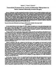
ˇ The actual expressions of g˜1 and g˜2 depend on which of the two Caplygin forms (20) or (21) applies. For example, if model (20) is used, we have g˜1 = α1 tan q3 and g˜2 = β1 sec q3 . In both cases, no closed-form is available for the solution of eq. (36), and the variation of q˙b along BC and DA as a function of U2 must be computed numerically. For illustration, Fig. 4 shows the relationship between U2 and the variation of q˙b = q˙2 obtained for model (20), with the dynamic parameters given in Sect. 6.1. Based on these considerations, we can determine the parameter values U1∗ , U2∗ that yield the desired reconfiguration according to the following procedure: 1. With the aid of Fig. 4, select U2∗ so as to obtain the desired variation −q˙bI for q˙b along BC and DA (and hence along the cycle). At this point, compute the corresponding variation q¯b for qb along BC and DA via forward integration of eq. (36). 2. By using the closed-form expression for qb (t) along AB and CD (i.e., the solution of eq. (35)), determine U1∗ so that the variation of qb along AB and CD equals qbd − qbI − q¯b . In this way, qb will attain the desired value qbd at the end of the cycle. To complete the analysis, we note the following points: • If no variation of q˙b is required (i.e., if q˙bI = 0), Fig. 4 would suggest to set U2 = 0. This choice, however, is not feasible, because any value of U1 would give no variation for qb at the end of the cycle. Therefore, in this case it is necessary to perform two cycles in the second phase giving velocity variations of equal magnitude and opposite sign. 20
• Assume that there exists an upper bound on the magnitudes U1 and U2 of the acceleration, e.g., U1max = U2max = 1 (the actual units depend on which of the ˇ two Caplygin forms (20) or (21) is being used). From Fig. 4, it appears that the maximum attainable variation for q˙b in this case is about 0.12 m/sec. If a larger variation is needed, i.e., if |q˙bI | > 0.12 m/sec, we must perform multiple cycles. • Realistic bounds on U1 and U2 depend—through eq. (7)—on the maximum applicable cartesian forces F . In particular, as the system approaches the singularities of the control law, these bounds become smaller, and a larger number of cycles will be required in order to achieve the desired reconfiguration. In view of this, it is advisable to choose in advance the size of the cycles in such a way that the singularity regions are avoided. For example, with model (20) one should stay away from values of q3 close to π/2.
6.1
Simulation results
The proposed approach has been simulated for a PPR robot having all links of unit mass and a uniform thin rod of length 2 m as third link. We present only the results of the second phase, which is the most interesting. Suppose that at the end of the first phase, the joint configuration is q I = (0, 0.5, 0) [m,m,rad] with velocity q˙I = (0, 0.05, 0). The final desired state at time 4δ = 8 sec is q d = q˙d = (0, 0, 0). The desired joint reconfiguration corresponds to an end-effector displacement from (3.5,2.5) to (3.5,2), due to the offset (1.5,2) on the prismatic joints. For this task, the joint vector must be partitioned as qa = (q1 , q3 ) and qb = q2 . Correspondingly, the system is put in the form (20) via feedback. A careful examination of Fig. 4 shows that the required variation of −0.05 m/sec for q˙2 is obtained for U2∗ ≈ −0.80 rad/sec2 . This introduces a net variation q¯2 for q2 along sides BC and DA approximately equal to −0.07 m. As a result, the total variation needed for q2 is −0.43 m/sec2 The desired value of U1 is then easily computed as U1∗ = −0.43 m/sec2 . The trajectories of the joint variables along the rectangular cycle are shown in Fig. 5, while the corresponding cartesian forces F acting on the end-effector are given in Fig. 6. A stroboscopic representation of the arm motion is shown in Fig. 7, together with the end-effector trajectory corresponding to the rectangle in the qa space. Points A# , B # , C # , D# and E # are respectively the cartesian-space images of the corners A, B, C, D, and A again. As expected, the closed rectangular trajectory in the qa space does not correspond to a closed path in the cartesian space.
21
7
Conclusions
An analysis of redundant robots driven by end-effector generalized forces has been performed by using tools from nonlinear controllability theory. We have identified conditions under which such systems may be cast into second-order triangular or ˇ Caplygin forms, and we have exploited these particular structures in order to design an end-effector steering algorithm that achieves a desired joint reconfiguration in finite time. The PPR planar robot was used as a case study to illustrate the proposed approach. We are currently considering the design of feedback controllers to perform the reconfiguration in a more robust fashion, as well as the application of our technique to more complex redundant robots. Furthermore, it would be desirable to gain more insight into the structure of the controllability conditions, in order to relate them to the dynamic properties of the mechanism. To this end, useful indications may be obtained by investigating the integrability properties of the underlying second-order differential constraint. Finally, the tools introduced in this paper with reference to a special class of underactuated mechanical systems might prove beneficial also in more general cases. In particular, both the nonlinear controllability analysis and the reconfiguration algorithm are quite naturally applicable to underactuated robots (De Luca et al., 1996).
Acknowledgments This work was partially supported by ESPRIT BR Project 6546 (PROMotion).
References Arai H. and Tachi S. (1991): Position control system of a two degree of freedom manipulator with a passive joint. — IEEE Trans. on Industrial Electronics, v.38, pp.15–20. Bianchini R. M. and Stefani G. (1993): Controllability along a trajectory: A variational approach. — SIAM J. on Control and Optimization, v.31, No.4, pp.900– 927. Bicchi A., Melchiorri C. and Balluchi D. (1995): On the mobility and manipulability of general multiple limb robots. — IEEE Trans. on Robotics and Automation, v.11, No.2, pp.215–228. Bloch A. M., Reyhanoglu M. and McClamroch N. H. (1992): Control and stabilization of nonholonomic dynamic systems. — IEEE Trans. on Automatic 22
Control, v.37, No.11, pp.1746–1757. Brockett R. W. (1983): Asymptotic stability and feedback stabilization, In: Differential Geometric Control Theory (R. W. Brockett, R. S. Millman, and H. J. Sussmann, Eds.). — Boston: Birkh¨auser. Campion G., d’Andrea-Novel B. and Bastin G. (1991): Modelling and state feedback control of nonholonomic mechanical systems. — Proc. 30th IEEE Conf. Decision and Control, Brighton, pp.1184–1189. Canudas de Wit C. and Sørdalen O. J. (1992): Exponential stabilization of mobile robots with nonholonomic constraints. — IEEE Trans. on Automatic Control, v.37, No.11, pp.1791–1797. Coron J.-M. (1992): Links between local controllability and local continuous stabilization. — Proc. Symp. Nonlinear Control Systems Design, Bordeaux, pp.477–482. De Luca A. and Oriolo G. (1994): Nonholonomy in redundant robots under kinematic inversion. — Proc. 4th IFAC Symp. Robot Control, Capri, pp.179–184. De Luca A. and Oriolo G. (1995): Modelling and control of nonholonomic mechanical systems, In: Kinematics and Dynamics of Multi-body Systems, (J. Angeles and A. Kecskem´ethy, Eds.). — Wien: Springer-Verlag. De Luca A., Mattone R. and Oriolo G. (1996): Control of underactuated mechanical systems: Application to the planar 2R robot. — Proc. 35th IEEE Conf. Decision and Control, Kobe. Goldstein H. (1980): Classical Mechanics. — Reading: Addison-Wesley. Hauser J. and Murray R. M. (1990): Nonlinear controllers for non-integrable systems: The Acrobot example. — Proc. American Control Conf., San Diego, pp.669–671. Isidori A. (1995): Nonlinear Control Systems. — London: Springer-Verlag. Kailath T. (1980): Linear Systems. — Englewood Cliffs: Prentice-Hall. Kolmanovsky I. V., Reyhanoglu M. and McClamroch N. H. (1994): Discontinuous feedback stabilization of nonholonomic systems in extended power form. — Proc. 33rd IEEE Conf. Decision and Control, Lake Buena Vista, pp. 3469– 3474. Laumond J.-P. (1990): Nonholonomic motion planning versus controllability via the multibody car system example. — Tech. Rep. STAN-CS-90-1345, Stanford University. 23
Lynch K. M. and Mason M. T. (1995): Controllability of pushing. — Proc. IEEE Conf. Robotics and Automation, Nagoya, pp.112–119. Murray R. M. and Sastry S. S. (1993): Nonholonomic motion planning: Steering using sinusoids. — IEEE Trans. on Automatic Control, v.38, No.5, pp.700– 716. Murray R. M., Li Z. and Sastry S. S. (1994): A Mathematical Introduction to Robotic Manipulation. — Boca Raton: CRC Press. Murray R. M. and M’Closkey R. T. (1995): Converting smooth, time-varying, asymptotic stabilizers for driftless systems to homogeneous, exponential stabilizers. — Proc. 3rd European Control Conference, Rome, pp.2620–2625. Neimark J. I. and Fufaev F. A. (1972): Dynamics of Nonholonomic Systems. Translations of Mathematical Monographs, v.33. — Providence: American Mathematical Society. Oriolo G. and Nakamura Y. (1991): Control of mechanical systems with secondorder nonholonomic constraints: Underactuated manipulators. — Proc. 30th IEEE Conf. Decision and Control, Brighton, pp.2398–2403. Samson C. (1993): Time-varying feedback stabilization of a car-like wheeled mobile robot. — Int. J. of Robotics Research, v.12, No.1, pp.55–64. Sørdalen O. J., Nakamura Y. and Chung W. J. (1994): Design of a nonholonomic manipulator. — Proc. IEEE Conf. Robotics and Automation, San Diego, pp.8–13. Spong M. W. (1995): The swing up control problem for the Acrobot. — IEEE Control Systems, v.15, No.1, pp.49–55. Sussmann H. J. (1987): A general theorem on local controllability. — SIAM J. on Control and Optimization, v.25, pp.158–194. Umetani Y. and Yoshida K. (1989): Resolved motion rate control of space manipulators with generalized jacobian matrix. — IEEE Trans. on Robotics and Automation, v.5, No.3, pp.303–314. Wichlund K. Y., Sørdalen O. J. and Egeland O. (1995): Control properties of underactuated vehicles. — Proc. IEEE Conf. Robotics and Automation, Nagoya, pp.2009–2014.
24
q3
q2
q1
Figure 1. A planar PRR robot
25
( px , py )
( px , py ) ! q3
q1
q2
Figure 2. A planar PPR robot
26
qa2
D
u1 = U1 u2 = 0
u 1 = – U1 u2 = 0
C
u1 = 0 u2 = – U2
u1 = 0 u2 = – U2
u1 = 0 u2 = U2
u1 = 0 u2 = U2
A
u 1 = – U1 u2 = 0
u1 = U1 u2 = 0
B qa1
Figure 3. A rectangular trajectory in the qa variables
27
0.15
variation of q2 velocity (m/s)
0.1
0.05
0
-0.05
-0.1
-0.15 -1
-0.8
-0.6
-0.4
-0.2
0 0.2 U2 (rad/s^2)
0.4
0.6
Figure 4. Variation of q˙b = q˙2 after one cycle as a function of U2
28
0.8
1
0.8 0.6
q2
joint variables (m,rad)
0.4 0.2 0 -0.2 -0.4
q1 -0.6
q3
-0.8 -1
0
1
2
3
4
5
6
7
time (s)
Figure 5. Evolution of the joint variables along the cycle
29
8
9
2
1.5
cartesian forces (N)
1
0.5
0
Fy
-0.5
-1
Fx -1.5
-2
0
1
2
3
4
5
6
7
8
time (s)
Figure 6. Cartesian forces acting on the end-effector along the cycle
30
9
4
3
B' A'
2
E' C'
1
D' 0
-1
-2
-3 -3
-2
-1
0
1
2
Figure 7. Arm motion along the cycle
31
3
4