Control Oriented Models for TWC-equipped Spark Ignition Engines during the Warm-up Phase Giovanni Fiengo1 , Luigi Glielmo2 , Stefania Santini3 , Gabriele Serra4 Abstract This paper introduces new phenomenological models of the spark ignition engine combustion and the threeway catalyst, able to describe the dynamic behaviors of the system in different operating modes, including the thermal transient, and being sufficiently simple for control synthesis. The models have been validated on experimental data.
1 Introduction In view of future stricter legislative thresholds on spark ignition engine (SI-engine) emissions, the modelling of the dynamical behavior of the cascade engine/threeway catalytic converter (TWC) becomes significant since the prediction of the transient allows the on-line optimization of engine fuelling strategies. In particular, this is necessary to minimize injurious emissions during the transient warm-up phase when the TWC is not working yet and, hence, a large amount of dangerous emissions is emitted in the air. In this paper new models of the the engine and the catalyst during the transient thermal phase will be presented . The goal of this modelling technique is to represent the dynamics of the overall systems behavior on a time scale of several engine events. In other words, the models are phenomenological, consistent, compact, with just a minimum number of fitting parameters, so as to be easily adaptable to different engines and sufficiently simple for control design. Having in mind to decouple the control of combustion from the control of 1 Giovanni Fiengo is PhD student, supported by Magneti Marelli Powertrain Division, Bologna, Italy, with Computer and System Engineering Department, Universit` a di Napoli Federico II, Naples, Italy. E-mail:
[email protected]. 2 Luigi Glielmo is with the School of Engineering, Universit` a del Sannio, Benevento, Italy. E-mail:
[email protected]. 3 Stefania Santini is with Computer and System Engineering Department, Universit` a di Napoli Federico II, Naples, Italy. Email:
[email protected]. 4 Gabriele Serra is with Magneti Marelli Powertrain Division, Bologna Italy. E-mail:
[email protected].
air manifold, we assumed as controllable inputs the flow of air and fuel into the cylinder and the spark advance. The outputs are the total unburned hydrocarbons pre and post converter.
2 Internal Combustion Engine In this paper a model of the internal combustion engine (ICE) is presented. The goal is to describe the transformation process of chemical energy into mechanical torque and heat, by combustion of air/fuel mixture and so the model does not include the dynamics of air and fuel across the manifold. The system inputs are the air mass flow rate (m ˙a [g/sec]) and air/fuel ratio (λ [/]) entering the cylinder; the spark advance (θ [deg]); the coolant temperature (Tcool [C]). Since the engine speed (n [rpm]) is determined by the driver commanding the torque, it is also considered in this model as an input. In the following, the blocks composing the whole engine model (see Figure 1) are presented. The first block, Burned fuel, computes the fuel charge (m ˙ fe [g/sec]) actually burned during the combustion. Here we suppose that only the air-fuel mixture that is in a stoichiometric ratio (14.6 part of air for 1 part of fuel) participates actively to the combustion process: if the air-fuel mixture is lean (λ ≥ 1) all the fuel in the cylinder takes part at the combustion; conversely, in rich condition (λ < 1), an amount of fuel equal to the 14.6-th part of the cylinder air is burned. Thus, the burned fuel is computed as follows 1 when λ ≥ 1 m ˙a λ × (λST = 14.6). m ˙ fe = λST 1 when λ < 1 (1) The block Combustion efficiency estimates the efficiency of the engine (ηf [%]) in transforming the chemical energy of the fuel into mechanical energy through combustion. We model as a product of two compo-
nents, ηλ and ηAV , as follows ¡ ¢ η λ = c 0 + θ c1 λ2 − c 2 λ , ∗ 2
(2a)
ηAV
=
1 − c3 (θ − θ ) ,
(2b)
ηf
=
ηλ · ηAV ,
(2c)
where θ ∗ is the nominal value of the spark advance for the production of the torque from the combustion; ηλ computes the combustion efficiency as a function of the engine operating point; ηAV modulates the combustion efficiency as a function of the distance between the real and the nominal value of the spark advance (θ−θ ∗ ). So (2b) is equal to 1 when θ is equal to θ ∗ and is less than 1 when it is different. The nominal value of the spark advance θ ∗ is computed as a function of the air mass flow rate m ˙ a , the engine speed n, and the coolant temperature Tcool , through the following black box model 30m˙ a 2 30m ˙a 3 30m˙ a + c6 ( ) + c7 ( ) + n n n 2 + c12 nTcool . (3) +c8 n + c9 n2 + c10 Tcool + c11 Tcool
θ ∗ = c4 + c5
The block Combustion estimates the effective torque generated by the combustion (T [Nm]): the mechanical power is computed multiplying the quantity of chemical energy generated by the combustion (m ˙ fe QHV , where QHV is the low heat value of the fuel [J/g]) and the combustion efficiency (ηf ); the effective torque is obtained dividing it for the engine speed, according to ηf m ˙ fe QHV . T = n
(4)
The quantity of energy generated by the combustion of the fuel and not transformed into effective power, (1 − ηf )m ˙ fe QHV , is dissipated as heat. A part of this thermal energy warms the engine mechanical components while the remaining part is transferred to the exhaust gas. Notice that, at the start, when the engine is cold, a large part of this heat goes toward the engine (approximately 75% of the total dissipated heat). Once warmed up, we assume that half of the heat is directed toward the engine and half to the exhaust gas. More precisely, we assume the coefficient β, describing this time-varying partition of thermal energy, to have the following dynamics 1 1 ˙ β(t) = − β(t) + . 75 150
(5)
The initial value of β, at cold start, is β(0) = 14 and the steady state value, reached after about 300sec, is β∞ = 21 ; the time constant is the same of the coolant. Thus, the heat produced by the combustion (Q˙ u [W]) warming the exhaust gas can be obtained as Q˙ u = β(t) (1 − ηf ) m ˙ fe QHV .
(6)
Figure 1: internal combustion engine
The block Thermal dynamics models the dynamical behavior of the exhaust gas temperature [1, 2]. The inputs of this block are the heat flow (Q˙ u ) generated by combustion (6), the coolant temperature (Tcool ) and the engine speed (n). T˙FG = a0 Q˙ u − a1 n(TFG − Tcool ).
(7)
Finally, the unburned hydrocarbons are calculated, in the rightmost block, as a function of the feedgas temperature TFG , air mass flow rate m ˙ a , spark advance θ, engine speed n and air/fuel ratio λ through the following black box model [3] ¡ ¢ T HCpre = b0 θ2 + b1 θ + b2 TFG + b3 λ2 − 2λ + +b4 n + b5 m ˙ a.
(8)
2.1 Identification results The parameters (a0 , a1 , bj for j = 0, . . . , 5, ck for k = 0, . . . , 12) in the previous equations were identified through a classic recursive least square [4]. The experimental data utilized for the identification and validation process refer to a Volkwagen Golf 1.6 engine performing an ECE (Economic Commission for Europe) drive cycle. In the next figures the results of the identification process are showed. The dotted line represents the real data and the solid line the simulation result. The nominal value of the spark advance θ ∗ and the combustion efficiency ηf during the ECE cycle are shown in Figures 2 and 3. Once the combustion efficiency is identified, it is possible to compute the heat generated by the combustion and directed to the exhaust gas Q˙ u , and the effective torque T . The latter is shown in Figure 4. In Figures 5 and 6 the temperature of the exhaust gas TFG and the unburned hydrocarbons T HCpre produced by the combustion during the ECE cycle are represented.
100 35
90 30
80 25
70
60 T [Nm]
15
*
θ [deg]
20
10
50
5
40
0
30
−5
20
−10
10 0
50
100
150 Time [sec]
200
250
300
0
50
Figure 2: Nominal value of the spark advance (θ ∗ )
100
150 Time [sec]
200
250
300
Figure 4: Effective torque T
0.55
450
0.5
400
0.45
350
0.4
300
[°C]
f
η [%]
0.35
250
T
FG
0.3 0.25
200
0.2
150
0.15
100
0.1
50 0
50
100
150 Time [sec]
200
250
300
Figure 3: Combustion efficiency ηf
0
0
50
100
150
200
250 Time [sec]
300
350
400
450
500
Figure 5: Exhaust gas temperature TFG
3 Three Way Catalytic Converter In literature some simplified model of a warmed-up catalyst are presented (see, for example, [5, 6, 7]). Even though based on the same approach, all these basic phenomenological models differ significantly in their internal structure, dynamic equations and state variable definition. In the following we present a TWC model aimed at describing the TWC behavior in every working condition, also including the warm-up phase. In current catalytic converters the presence of Cerium improves the performance by allowing the oxygen storage phenomenon [8, 9]: during transients, in presence of oxygen excess, there is an oxygen chemiadsorption on the catalyst, while in conditions of defect, there is a release. In other words, if an excess of O2 participates in the combustion, it will be chemically stored (up to
a certain capacity); conversely, if a deficit of O2 exists then the catalyst will give up oxygen (as long as some is available) to allow the reactions to happen. Thus, the oxygen-storage is a key mechanism that enhances the catalyst activity helping the catalyzed oxidationreduction reactions. The model is an improvement of a our previous work presented in [7]. In Figure 7 a block diagram of the model is shown: the block Oxygen storage models the above-mentioned phenomenon and the chemical process of the unburned hydrocarbons oxidation is described in the block Catalytic Reactions. In the next sections the two sub-models are presented, and the identification results can be found in the last section.
0.035
per unit of time is computed as ½ fL (Θ) ˙ ˙ ˙ Θcor = (ΘFG − ΘSt )·g(TFG )· fR (Θ)
whenλFG ≥ 1 whenλFG < 1 (10) ˙ FG − Θ ˙ St ) is the fraction of oxygen capacity where (Θ that is available for the storage or requested by the catalytic reactions per unit of time; Θ is the fraction of oxygen capacity occupied in the TWC; TFG [C] is the feedgas temperature affecting the TWC efficiency by means of function g(TFG ), switching around a threshold value Tth , according to
0.03
THCpre [g/sec]
0.025
0.02
0.015
0.01
0.005
0
50
100
150 Time [sec]
200
250
300
g(TFG ) =
tanh[(TFG − Tth )γ] + 1 ; 2
γ is a parameter to be identified; the functions fL (Θ) and fR (Θ) determine how much of the surplus or deficit oxygen can be respectively stored or released, according to
Figure 6: Unburned hydrocarbons T HCpre
fL (Θ) fR (Θ)
Figure 7: Three way catalytic converter
3.1 Oxygen Storage The oxygen storage phenomenon is modelled by two actions aimed at correcting the quantity of oxygen in the gas at the inlet of the catalyst, trying to reach the optimal value for the catalytic reactions, the stoichiometric point. In other word, during the lean condition, the excess of oxygen from the optimal value is stored, while, in rich condition, the quantity of oxygen necessary to reach the optimal point is released. Let us denote the fraction per unit of time of the total oxygen quantity present in the feedgas and, ideally, at the stoichiometric value respectively by ˙ FG Θ ˙ St Θ
= =
0.23 m ˙ f λFG S , C 0.23 m ˙ fS , C
(11)
where m ˙ f [g/sec] is the fuel mass flow rate; λFG [/] is the air-fuel ratio at the feedgas; S is the stoichiometric value (∼ 14.6); 0.23 is the mass percentage of oxygen present in the air; C [g] is the capacity of the catalyst. The fraction of oxygen capacity that is effectively stored in lean condition or released in rich condition
(1 − Θ8 ), [1 − (1 − Θ)8 ].
(12a) (12b)
Notice that, in lean condition, if the catalyst is full (θ = 1) the oxygen cannot be stored (fL = 0); conversely, if the catalyst is empty (θ = 0) all the oxygen available can be stored (fL = 1). Conversely, in rich condition, when the catalyst is full (θ = 1) all the deficit oxygen can be released (fR = 1) and if it is empty (θ = 0) it is not possible to release oxygen (fR = 0). Moreover, if the temperature TFG is lower than the threshold (Tth ) nothing happens (g(TFG ) ' 0), conversely if it is bigger the oxygen storage phenomenon is active (g(TFG ) ' 1). ˙ cor is evaluated, we can compute the fraction Once Θ of oxygen capacity per unit of time in the gas after ˙ FG , and the corresponding A/F this first correction, Θ cor ratio, λFGcor : ˙ FG Θ cor
=
λFGcor
=
˙ FG − Θ ˙ cor , Θ ˙ ΘFGcor C . 0.23 m ˙ fS
(13a) (13b)
By phenomenological considerations, here the second correction is modelled by a first order system
(9a) (9b)
= =
λ˙ aux = −
λFGcor λaux + , (14) τ (λFG , λaux , TFG ) τ (λFG , λaux , TFG )
where τ (λFG , λaux , TFG ) is the time constant, depending on the air/fuel ratio of the gas at the inlet and the outlet of the catalyst, and the feedgas temperature. In particular this action is more significant when the air fuel ratio of the gas at the TWC inlet is closed to the stoichiometry and temperature is bigger than the activation threshold. This is described by the time
constant that in this conditions reaches its maximum value. The corresponding fraction of oxygen capacity per unit of time presents in the gas at the outlet of the catalyst ˙ aux is computed as Θ ˙ f λaux S ˙ aux = 0.23 m . Θ C
(15)
Hence, the fraction of oxygen capacity that is altogether stored or released from the TWC per unit of time is simply the difference between the oxygen frac˙ FG and the oxygen fraction in the tion in the feedgas Θ ˙ aux . The change of oxygen gas after the two actions Θ capacity occupied in the TWC is ˙ FG − Θ ˙ aux when Θ ∈ (0, 1) Θ ˙ ˙ FG − Θ ˙ aux } Θ= max{0, Θ when Θ = 0 ˙ FG − Θ ˙ aux } min{0, Θ when Θ = 1 (16) Finally the air-fuel ratio at the tailpipe, λTP is computed as λTP (t) = λaux (t − ∆(t)), (17) where ∆ is the transport delay of the gas, depending f on an average value m ˙ a of the air mass flow rate ∆(t) =
δ1 + δ2 . f m ˙ a (t)
(18)
The coefficient C, Tth , γ, δ1 , δ2 , τmin and τmax have to be identified for each specific catalytic converter. 3.2 Catalytic Reactions In this section a phenomenological model of the reactions taking place in the TWC is presented. In particular it models only the un unburned hydrocarbons oxidation since it is the most relevant process during the warm-up phase. The total hydrocarbons (THC) in the exhaust gas are divided into two groups: ‘fast oxidizing hydrocarbons’ and ‘slow oxidizing hydrocarbons’. In this model the former group is represented by propylene (C3 H6 ) and the latter by methane (CH4 ) and we considered the propylene to constitute 86% of the THC and methane the remaining 14%. They participate in the reactions C3 H6 + 4.5O2 CH4 + 2O2
→ 3CO2 + 3H2 O, → CO2 + 2H2 O.
(19a) (19b)
The kinetic model has one output (the mass flow rate of the unburned hydrocarbons at the outlet of the TWC, T HCpost [g/sec]), five inputs (the mass flow rate of the unburned hydrocarbons at the inlet of the TWC, THCpre [g/sec]; the engine speed, n [rpm]; the fuel
flow rate, m ˙ f [g/sec]; the air/fuel ratio of the gas corrected by the oxygen storage phenomenon, λTP [/]; the feedgas temperature, TFG [C]). It is supposed to divided the TWC in two parts connected in series: the unburned hydrocarbons produced by the engine combustion enter in the first part of the TWC and there the first oxidation reactions take place; the remaining unburned hydrocarbons, called T HCmd , pass through the first part in which is divided the TWC and arrive in the second part, where other oxidation reaction take place. The unburned hydrocarbons, not oxidized in the two part of the TWC, called T HCpost , are the output of the system. In conclusion, the model is composed of two states (the mass flow rate of the unburned hydrocarbons in the middle of the catalyst, THCmd [g/sec] and at the end, THCpost [g/sec]) as follows ˙ md = −K1 n(THCmd − THCpre ) + THC −Rmd (TFG , THCmd , m ˙ f , λTP ),
(20a)
˙ post = −K2 n(THCpost − THCmd ) + THC −Rpost (TFG , THCpost , m ˙ f , λTP ));
(20b)
where the reaction rates Ri (TFG , THCi , m ˙ f , λTP ), i = md, post, have the form [10] p ˙ f λTP × Ri (TFG , THCi , m ˙ f , λTP ) = Ki THCi m tanh[(TFG − Tthi )γi ] + 1 . × 2 The coefficients K1 , K2 , Kmd , Kpost , Tthmd , Tthpost , γmd , γpost have to be identified. 3.3 Identification results A stochastic procedure, using both a purposely genetic algorithm (e.g. see [11]) and a least square optimization, has been designed to identify the coefficients of the catalytic converter model. The experimental data utilized for the identification and validation process again refer to a Golf 1.6 performing an ECE cycle. In Figure 8 the air/fuel ratio of the exhaust gas at the input (dotted line) and the output (solid line) of the catalyst are plotted. It is apparent that the model well captures the main behavior of the TWC; in particular the oxygen storage phenomenon does not occur when the catalyst is not sufficiently hot (λTP ' λFG ), while after TWC light off the oxygen storage becomes significant especially if the mixture is close to stoichiometry. Finally, Figure 9 shows the unburned hydrocarbons at the input of the TWC (dashed line), the real output (dotted line) and simulated output (solid line).
4 Conclusions In this paper control oriented models of SI engine and three-way catalyst were presented. The models, which
References [1] J. A. Kaplan and J. B. Heywood, “Modelling the spark ignition engine warm-up process to predict component temperatures and hydrocarbon emissions,” SAE paper, , no. 910302, 1991.
1.15
1.1
λ [/]
1.05
[2] I. K. Yoo, K. Simpson, M. Bell, and S. Majkowski, “An engine coolant temperature model and application for cooling system diagnosis,” SAE paper, , no. 2000-01-0939, 2000.
1
0.95
0.9
[3] U. Grezzi and C. Ortolani, Combustione e Inquinamento, Tamburini Editore, 1974.
0.85
0.8
0
50
100
150
Time [sec]
Figure 8: Air/Fuel ratio at the inlet and outlet of the TWC λFG
[7] G. Fiengo, L. Glielmo, and S. Santini, “On board diagnosis for three-way catalytic converters,” International Journal of Robust Nonlinear Control, vol. 11, pp. 1073–1094, 2001.
0.02
THC [g/sec]
[5] E. P. Brandt, Y. Wang, and J. W. Grizzle, “Dynamic modeling of a three-way catalyst for si engine exhaust emission control,” IEEE Trans. on Control System Technology, vol. 85, pp. 767–776, 2000. [6] J. C. Jones, R. A. Jackson, J. B. Roberts, and P. Bernard, “A simplified model for the dynamics a three-way catalytic converter,” SAE paper, , no. 200001-0652, 2000.
0.025
0.015
[8] H. C. Yao and Y. F. Yu Yao, “Ceria in automotive exhaust catalysts. oxygen storage,” Journal Catalysis, vol. 86, pp. 254–265, 1984.
0.01
0.005
0
[4] S. Bittanti, Identificazione dei modelli e controllo adattativo, Pitagora Editrice, 1997.
0
50
100
150 Time [sec]
200
250
300
Figure 9: Unburned hydrocarbons at the inlet and outlet of the TWC (T HC)
[9] E. C. Su, C. N. Montreuil, and W. G. Rothschild, “Oxygen storage capacity of monolith three way catalysts,” Applied Catalysis, vol. 17, pp. 75–86, 1985. [10] F. Aimard, S. Li, and M. Sorine, “Mathematical modeling of automotive three-way catalytic converters with oxygen storage capacity,” Control Engineering Practice, vol. 4, no. 8, pp. 1119–1124, 1996. [11] L. Davis, Handbook of Genetic Algorithms, Van Nostrand Reinhold, 1991.
have been identified and validated on experimental data, can be used for real-time control application, such as, for example, warm-up controllers. As an example, a control application based on these models can will be found in [12].
5 Acknowledgments The authors wish to thank dr. ing. Giuseppe Police of the Istituto Motori of CNR (Italian National Research Council) for helpful discussions.
[12] G. Fiengo, L. Glielmo, S. Santini, and G. Serra, “Control of the exhaust gas emissions during the warmup procress of a twc-equipped si-engine,” accepted for International Federation of Automatic Control 15th World Congress, Barcelona, Spain, 2002.