Control 2004, University of Bath, UK, September 2004
ID-061
Control Performance of a Real-time Adaptive Distributed Control System under Jitter Conditions Ana Antunes*, Alexandre Manuel Mota † *Escola Superior de Tecnologia de Setúbal, Instituto Politécnico de Setúbal, Portugal, Campus do IPS, Estefanilha, 2914-508 Setúbal, Tel: (351)265790000, Fax: (351)265721869,
[email protected] † Departamento de Electrónica e Telecomunicações, Universidade de Aveiro, Portugal, Campus Universitário de Santiago, 3810-193 Aveiro, Tel: +351 234370383,Fax: +351 234381128,
[email protected]
Keywords: jitter, control performance, real-time distributed control systems, adaptive controller.
Abstract In this paper it is made an analysis of the control performance of a pole-placement adaptive controller for a real-time distributed control system under output jitter conditions using different models of the plant. Two models were used with and without taking into account the fractional dead-time to model jitter effect.
Plant
Sensor node (S)
Controller node (C)
Actuator node (A)
CAN bus
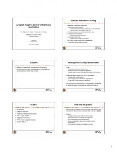
Figure 1: Block diagram of the distributed control system. M1
1 Introduction Nowadays distributed control systems are widely used in embedded applications. It is well known that distributed control architectures induce jitter, either in the sampling period (called input jitter, sampling jitter or read-in jitter) or in the actuation moment (called sampling to actuation jitter, output jitter or read-out jitter) eventually leading to performance degradation [1],[6],[12],[13],[14]. In [4] and [5] it is proposed a method for modelling and identifying systems subject to jitter that takes under consideration a fractional dead-time with a value equal to the jitter average to model jitter effects. This paper presents a comparison between the control performance of the real-time distributed control system under jitter conditions obtained using identification models with and without taking the fractional dead-time into account. The results show that, using the model with fractional dead-time, the overall system remains stable even when subject to severe jitter conditions.
2 The system The block diagram of the real-time distributed control system is shown in figure 1. The system has three nodes: the sensor node, the controller node and the actuator node. The nodes are connected using the CAN bus. The communication scheme is shown in figure 2. The sensor node sends a message (M1) with the sampled value to the controller node that computes the actuation value for the next sample and sends that value and the actuation order (M2) to the actuation node.
S
C C
A M2
Figure 2: Communication model scheme for the system. The system was simulated using TrueTime a MATLAB/Simulink based simulator for real-time control systems [2],[3],[8]. The simulator facilitates co-simulation of controller task execution in real-time kernels, network transmissions and continuous plant dynamics. This tool was chosen because of its flexibility and ease of use that allows the test of different system conditions easily. Each node of the system was implemented using a TrueTime Kernel block and the CAN bus was implemented with a TrueTime Network block [7]. The plant models a cruise control system and its transfer function is given by equation (1). 0.05 Y (s) = U ( s ) s + 0.05
(1)
This model was taken from [15].
3 The adaptive controller The system controller used was an adaptive controller. The adaptive controller block diagram is shown in figure 3 [9]. The adaptive controller has two loops. The inner loop includes the variable dynamics controller and the process.
Control 2004, University of Bath, UK, September 2004
ID-061
Process Parameters
Specification
G (q ) = [1 Design
This leads to equations (12) and (13) for models 1 and 2, respectively.
Controller
Process Output
Input
Figure 3: Block diagram of the adaptive controller. The outer loop is composed by the recursive process parameter estimator and a design calculator block and is responsible for the adjustment of the parameters of the controller. The controller was implemented in MATLAB inside the TrueTime Kernel of the controller node. 3.1 System identification The generic form of the discrete time transfer function is given by equation (2). G (q −1 ) = z − K
(11)
Estimation
Controller Parameters Reference
0](qI − Φ ) −1 (Γ0 + Γ1 q −1 )
B(q −1 ) A(q −1 )
(2)
−1
−1
B(q ) = b0 + b1q + K + bm z
−m
dx(t ) = Ax (t ) + Bu (t − τ ) dt y (t ) = x(t )
(4)
(5) (6)
where τ represents the variable delay which can be considered as a dead-time. If that delay is bounded by the sampling period h (τ