Distributed Adaptive Control for Networked Multi

3 Distributed Adaptive Control for Networked Multi-Robot Systems Abhijit Das and Frank L. Lewis

Automation and Robotics Research Institute, University of Texas at Arlington, Fort Worth USA 1. Introduction

Synchronization behavior among agents is found in flocking of birds, schooling of fish, and other natural systems. Synchronization among coupled oscillators was studied by (Kuramoto 1975). Much work has extended consensus and synchronization techniques to manmade systems such as UAV to perform various tasks including surveillance, moving in formation, etc. We refer to consensus and synchronization in terms of control of manmade dynamical systems. Early work on cooperative decision and control for distributed systems includes (Tsitsiklis 1984). The reader is referred to the book and survey papers (Ren & Beard 2008; Ren, Beard et al., 2005; Olfati-Saber et al., 2007; Ren, Beard et al., 2007). Consensus has been studied for systems on communication graphs with fixed or varying topologies and communication delays. See (Olfati-Saber & Murray 2004; Fax & Murray 2004; Ren & Beard 2005; Jadbabaie et al., 2003), which proposed basic synchronizing protocols for various communication topologies. Early work on consensus studied leaderless consensus or the cooperative regulator problem, where the consensus value reached depends on the initial conditions of the node states and cannot be controlled. On the other hand, the cooperative tracker problem seeks consensus or synchronization to the state of a control or leader node. Convergence of consensus to a virtual leader or header node was studied in (Jadbabaie et al., 2003; Jiang & Baras 2009). Dynamic consensus for tracking of time-varying signals was presented in (Spanoset al., 2005). The pinning control has been introduced for synchronization tracking control of coupled complex dynamical systems et al., 2004; Z. Li et al., 2009). Pinning control allows controlled synchronization of interconnected dynamical systems by adding a control or leader node that is connected (pinned) into a small percentage of nodes in the network. Analysis has been done using Lyapunov and other techniques by assuming either a Jacobian linearization of the nonlinear node dynamics, or a Lipschitz condition, or contraction analysis. The agents are homogeneous in that they all have the same nonlinear dynamics. The study of second-order and higher-order consensus is required to implement synchronization in most real world applications such as formation control and coordination among UAVs, where both position and velocity must be controlled. Note that Lagrangian motion dynamics and robotic systems can be written in the form of second-order systems. Moreover, second-order integrator consensus design (as opposed to first-order integrator node dynamics) involves more details about the interaction between the system dynamics/ control design problem and the graph structure as reflected in the Laplacian matrix. As

34

Multi-Robot Systems, Trends and Development

such, second-order consensus is interesting because there one must confront more directly the interface between control systems and communication graph structure. See the book (Ren & Beard 2008) in Section III (Chapter 4-5). The article (Ren et al., 2007) studied the case of higher-order consensus for linear chained integrator systems. The detailed analysis there is performed for 3rd order systems but it extends to the higher order case. The paper (Zhu et al., 2009) studies the general second order consensus problem for double integrator systems. Ref. (Khoo et al., 2009) studied second order consensus in finite time using sliding mode error and a Lyapunov analysis. Papers (Bo & Huajing 2009; Yang et al., 2008; Su & Xiaofan Wang 2008) discuss consensus with time delays for second order integrator (Type II) systems. The article (Seo et al., 2009) proposed second order consensus using output feedback for agents with identical linear dynamics. Few papers study second-order consensus for unknown nonlinear systems. Few papers study consensus for heterogeneous agents with different unknown nonlinear dynamics. Leaderless or uncontrolled synchronization with nonlinear non-identical passive systems is reported in (Chopra & Spong 2006), which provided a Lyapunov proof valid for balanced graph structures. By contrast, this Chapter concerns controlled consensus or the multi-agent tracker problem on general directed graphs. Neural networks (NN) have a universal approximation property (Hornik et al., 1989) and learning capabilities that make them ideal for cooperative tracking control of multi agent systems with non-identical unknown nonlinear dynamics. Neural networks have been used since the 1990s to extend the abilities of adaptive controllers to handle larger classes of unknown nonlinear dynamical systems. Novel NN weight tuning algorithms have been developed to make NN suitable for online control of dynamical systems with real-time learning along the system trajectories. Rigorous proofs of convergence, performance, and stability have been offered. The reader is referred to (Qu 2009; Lewis et al., 1999; Lewis et al., 1996; Narendra 1992; Narendra & Parthasarathy 1990; F. -C Chen & Khalil 1992; Polycarpou 1996) for early works and the extensive literature since then is well known and hence not covered here. Neural adaptive control has not been fully explored for control of multiagent systems. Distributed multiagent systems with unknown nonlinear non-identical dynamics and disturbances were studied in (Hou et al., 2009) where distributed neural adaptive controllers were designed to achieve robust consensus. That treatment assumed undirected graphs and solved the leaderless or uncontrolled consensus problem, that is, the nodes reach a steadystate consensus that depends on the initial conditions and cannot be controlled. Expressions for the consensus value were not given. Higher order consensus was proposed using a complex backstepping approach. Many control system graph structures are nonsymmetric in that communication links are unidirectional, with information flowing only one way between subsystems. Moreover, in most problems it is important to be able to specify the desired synchronization trajectory. This corresponds to a multi-agent tracker problem. An example is the directed tree structure of formation control, where all agents sense (either directly or indirectly through intermediate neighbors) the state of the control node, but the control node sets the prescribed course and speed. Therefore, (Das & Lewis 2009) studied the cooperative tracker problem for agents on general digraphs having non-identical unknown dynamics and disturbances. First-order integrator dynamics were studied. A distributed adaptive control technique was given that used pinning control to achieve synchronization to a desired command trajectory. Performance and stability were shown using a Lyapunov approach.

35

Distributed Adaptive Control for Networked Multi-Robot Systems

In this Chapter we extend (Das & Lewis 2009) to consensus for agents having second order dynamics in Brunovsky form. We confront the second-order synchronization tracking problem for heterogeneous nodes with non-identical unknown nonlinear dynamics with unknown disturbances. Herein, ‘synchronization control’ means the objective of enforcing all node trajectories to follow (in a ‘close-enough’ sense to be made precise) the trajectory of a leader or control node. The communication structures considered are general directed graphs with fixed topologies. Analysis of digraphs is significantly more involved than for undirected graphs. The dynamics of the leader or command node are also assumed nonlinear and unknown. A distributed adaptive control approach is taken, where cooperative adaptive controllers are designed at each node. A parametric neural network structure is introduced at each node to estimate the unknown dynamics. The choices of control protocol as well as neural net tuning laws are the key factors in stabilizing the networked multi-agent systems. A Lyapunov analysis shows how to tune the neural networks cooperatively, and guarantees the stability and performance of the networked systems. The error bounds obtained from the Lyapunov proof are dependent on control design and NN tuning parameters which can be chosen to suitably manage the tracking error and estimation error. Simulation results for networked agents with Lagrangian dynamics are provided to show the effectiveness of the proposed method. Section 2 is formulated the synchronization tracking control problem for second-order systems with non-identical unknown nonlinear dynamics. In Section 3 a Lyapunov technique is used to design cooperative adaptive controllers based on neural network approximation methods. Performance and stability guarantees are given for the networked systems. Section 4 presents simulation results.

2. Synchronization control formulation Consider a graph G = (V , E) with a nonempty finite set of N nodes V = { v1 ," , vN } and a set of edges or arcs E ⊆ V × V . We assume the graph is simple, e.g. no repeated edges and ( vi , vi ) ∉ E , ∀i no self loops. General directed graphs are considered. Denote the adjacency or connectivity matrix as A = [ aij ] with aij > 0 if ( v j , vi ) ∈ E and aij = 0 otherwise. Note aii = 0 . The set of neighbors of a node vi is N i = { v j : ( v j , vi ) ∈ E} , i.e. the set of nodes with

arcs incoming to vi . Define the in-degree matrix as a diagonal matrix D = diag{ di } with di =

∑ aij

the weighted in-degree of node i (i.e. i -th row sum of A). Define the graph

j∈N i

laplacian matrix as L = D − A , which has all row sums equal to zero. Define dio = ∑ a ji , the j

(weighted) out-degree of node i , that is the i -th column sum of A . We consider directed communication graphs with fixed topologies and assume the digraph is strongly connected, i.e. there is a directed path from vi to v j for all distinct nodes vi , v j ∈ V . Then A and L are irreducible (Qu 2009), (Horn & Johnson 1994). That is they are not cogredient to a lower triangular matrix, i.e., there is no permutation matrix U such that ⎡* 0⎤ T L =U⎢ ⎥U ⎣* * ⎦

(1)

36

Multi-Robot Systems, Trends and Development

The results of this Chapter can easily be extended to graphs having a spanning tree (i.e. not necessarily strongly connected) using the Frobenius form in (1). 2.1 Cooperative tracking problem for synchronization of multiagent systems Consider second order node dynamics defined for the i -th node in Brunovsky form as x i1 = xi2

(2)

x i2 = f i ( xi ) + ui + wi

where xi = [ xi1 xi2 ]T ∈ R 2 , ui (t ) ∈ R is the control input and wi (t ) ∈ R a disturbance acting upon each node. Note that each node may have its own distinct nonlinear dynamics. Standard assumptions for existence of unique solutions are made, e.g. f i ( xi ) either continuously differentiable or Lipschitz. The overall graph dynamics is x 1 = x 2

(3)

x 2 = f ( x ) + u + w

where the overall (global) state vector is x 2 = ⎡⎣ x12 x 1 = ⎡⎣ x11

(

T

1 ⎤ N 1 2 x21 " xN ⎦ ∈ R , x = x ,x

input u = [ u1

)

T

T

2 ⎤ N x22 " xN ⎦ ∈R ,

, f ( x ) = ⎡⎣ f 1 ( x1 )

u2 " uN ] ∈ R N , and w = [ w1 T

f 2 ( x2 ) "

T

f N ( xN ) ⎤⎦ ∈ R N ,

w2 " wN ] ∈ R N . T

If the states xik are not scalars, this analysis carries over with the mere addition of the standard Kronecker product term (Das & Lewis 2009). Definition 1. The local neighborhood tracking synchronization errors (position and velocity) for node i are defined as (Khoo et al., 2009) ei1 =

∑ aij ( x1j − xi1 ) + bi ( x01 − xi1 )

(4)

∑ aij ( x 2j − xi2 ) + bi ( x02 − xi2 )

(5)

j∈N i

and

ei2 =

j∈N i

with pinning gains bi ≥ 0 , and bi > 0 for at least one i . Then, bi ≠ 0 if and only if there exist an arc from the control node to the i -th node in G . We refer to the nodes i for which bi ≠ 0 as the pinned or controlled nodes. Note that (4) and (5) represents the information that is available to any node i for control purposes. The state x0 = [ x01 x02 ]T ∈ R 2 of the leader or control node satisfies the (generally nonautonomous) dynamics in Brunovsky form x 01 = x02 x 02 = f 0 ( x0 , t )

(6)

37

Distributed Adaptive Control for Networked Multi-Robot Systems

This can be regarded as a command or reference generator. A special case is the standard constant consensus value with x 01 = 0 and x02 absent. Here, we assume that the control node can have a time-varying state. The Synchronization tracking control problem confronted herein is as follows: Design control protocols for all the nodes in G to synchronize to the state of the control node, i.e. one requires xik (t ) → x0k (t ), k = 1, 2, ∀i . It is assumed that the dynamics of the control node is unknown to any of the nodes in G . It is assumed further that both the node nonlinearities f i (.) and the node disturbances wi (t ) are unknown. Thus, the synchronization protocols must be robust to unmodelled dynamics and unknown disturbances. 2.2 Synchronization tracking error Define the consensus disagreement error vector T

δ = ⎡⎣δ 1 δ 2 ⎤⎦ = ⎡⎣ x 1 − 1 x01 x 2 − 1 x02 ⎤⎦

T

(7)

From (4), the global error vector for network G is given by

(

)

(8)

(

)

(9)

e 1 = − ( L + B) x 1 − 1 x01 = − ( L + B) δ 1 and e 2 = − ( L + B) x 2 − 1 x02 = − ( L + B) δ 2 where, B = diag{bi } is the diagonal matrix of pinning gains, and e k = ⎡⎣ e1k k = 1, 2, ∀i and 1 ∈ R N the vector of 1’s. Lemma 1. Let the graph is strongly connected and B ≠ 0 . Then

δ k ≤ e k / σ ( L + B) , with σ ( L + B) the minimum singular value of

k = 1, 2

( L + B) ,

T

k ⎤ N e2k " eN ⎦ ∈R ,

(10)

and e = 0 if and only if the nodes

synchronize, that is xik (t ) = x0k (t ), k = 1, 2, ∀i .

(11)

2.3 Synchronization Control Design and Error Dynamics Differentiating (8) and (9),

(

e 1 = − ( L + B ) x 2 − 1 x02

)

(12)

and

(

e 2 = − ( L + B ) x 2 − 1 f 0 ( x0 , t )

Note that e 1 = e 2 . Define sliding mode error for node i

)

(13)

38

Multi-Robot Systems, Trends and Development

or as a whole

ri = ei2 + λi ei1

(14)

r = e 2 + Λe 1

(15)

where Λ = diag(λi ) > 0 . The next result follows directly. Lemma 2. The velocity error is bounded according to e2 ≤ r + σ ( Λ ) e1

(16)

Now differentiating r one obtains the error dynamics

(

)

(

r = − ( L + B) x 2 − 1 f 0 ( x0 , t ) − Λ ( L + B ) x 2 − 1 x02

)

= − ( L + B) ( f ( x ) + u + w ) + ( L + B ) 1 f 0 ( x0 , t ) + Λe 2

(17)

Following the techniques in (Lewis et al., 1999; Ge et al., 1998), assume that the unknown nonlinearities in (2) are smooth and thus can be approximated on a compact set S ∈ R by f i ( xi ) = WiTϕi ( xi ) + ε i

(18)

with ϕi ( xi ) ∈ Rηi a suitable basis set of ηi functions at each node i with ηi number of neurons and Wi ∈ Rηi a set of unknown coefficients. According to the Weierstrass higherorder approximation theorem (Stone 1948), a polynomial basis set suffices to approximate f i ( xi ) as well as its derivatives, when they exist, and moreover, the approximation error ε i → 0 uniformly as ηi → ∞. According to the neural network (NN) approximation literature (Hornik et al., 1989), a variety of basis sets can be selected, including sigmoids, gaussians, etc. There ϕi ( xi ) ∈ Rηi is known as the NN activation function vector and Wi ∈ Rηi as the NN weight matrix. Then it is shown that ε i is bounded on a compact set. The ideal approximating weights Wi ∈ Rηi in (7) are assumed unknown. The intention is to select only a small number ηi of NN neurons at each node (see Simulations). Here, to avoid distractions from the main issues being introduced, we assume a linear-inthe-parameters NN, i.e. the basis set of activation functions is fixed and only the output weights are tuned. It is straightforward to use a two-layer NN whereby the first and secondlayer weights are tuned. Then one has a nonlinear-in-the-parameters NN and the basis set is automatically selected in the NN. Then, the below development can easily be modified as in (Lewis et al., 1999). To compensate for unknown nonlinearities, each node will maintain a neural network locally to keep track of the current estimates for the nonlinearities. The idea is to use the information of the states from the neighbors of node i to evaluate the performance of the current control protocol along with the current estimates of the nonlinear functions. Therefore, select the local node’s approximation fˆi ( xi ) as ˆ Tϕ ( x ) fˆi ( xi ) = W i i i

(19)

ˆ ∈ Rηi is a current estimate of the NN weights for node i , and η is the number of where W i i NN neurons maintained at each node i . It will be shown in Theorem 1 how to select the

39

Distributed Adaptive Control for Networked Multi-Robot Systems

ˆ ∈ Rηi using the local neighborhood synchronization errors estimates of the parameters W i (4), (5). The global node nonlinearity f ( x ) for graph G is now written as ⎡ W1T ⎢ ⎢ f ( x ) = W Tϕ ( x ) + ε = ⎢ ⎢ ⎢ ⎢ ⎣⎢

W2T

⎤ ⎡ ϕ (x ) ⎤ ⎡ ε ⎤ ⎥⎢ 1 1 ⎥ ⎢ 1 ⎥ ⎥ ⎢ ϕ 2 ( x2 ) ⎥ ⎢ ε 2 ⎥ ⎥⎢ # ⎥ + ⎢ # ⎥ % ⎥⎢ ⎥ ⎢ ⎥ ⎥⎢ # ⎥ ⎢ # ⎥ % ⎥⎢ ϕN ( xN )⎥⎦ ⎢⎣ε N ⎥⎦ WNT ⎦⎥ ⎣  

(20)

ϕ(x)

and the estimate fˆ ( x ) as ˆT ⎡W 1 ⎢ ⎢ ˆ Tϕ ( x ) = ⎢ fˆ ( x ) = W ⎢ ⎢ ⎢ ⎢⎣

ˆT W 2

⎤ ⎡ ϕ (x ) ⎤ ⎥⎢ 1 1 ⎥ ⎥ ⎢ ϕ 2 ( x2 ) ⎥ ⎥⎢ # ⎥ % ⎥⎢ ⎥ ⎥⎢ # ⎥ % ⎥ ˆ T ⎥ ⎢⎣ϕN ( xN )⎥⎦ W N ⎦  

(21)

ϕ(x)

Consider an input ui = − fˆi ( xi ) + μi ( x , t )

(22)

u = − fˆ ( x ) + μ ( x , t )

(23)

or

with μi ( x , t ) an auxiliary input for the i th node yet to be specified. Then using (12) the error dynamics (6) becomes

(

)

r = − ( L + B) f ( x ) + μ ( x , t ) + w + ( L + B) 1 f 0 ( x0 , t ) + Λe 2

(

ˆ ,W − W ˆ ,"" , W − W ˆ  = diag W − W  ϕ ( x ) with W where f ( x ) = f ( x ) − fˆ ( x ) = W N N 1 1 2 2

(24)

)

T

.

3. Lyapunov design for cooperative adaptive tracking control It is now shown how to select the auxiliary control μ (t ) and NN weight tuning laws such as to guarantee that all nodes synchronize to the desired control node signal, i.e., xi (t ) → x0 (t ), ∀i . It is assumed that the dynamics f ( x0 , t ) of the control node (which could represent its motion) are unknown to any of the nodes in G . It is assumed further that the node nonlinearities f i ( xi ) and disturbances wi (t ) are unknown. The Lyapunov analysis technique approach of (Lewis et al., 1999; Lewis et al., 1996) is used, though there are some complications arising from the fact that μ ( x , t ) and the NN weight tuning laws must be implemented as distributed protocols. This entails a careful selection of the Lyapunov function.

40

Multi-Robot Systems, Trends and Development

The maximum and minimum singular values of a matrix M are denoted σ ( M ) and σ ( M ) respectively. The Frobenius norm is M inner product of two matrices is M1 , M2

F F

= tr { M T M } with tr {} ⋅ the trace. The Frobenius = tr { M1T M2 } .

The following Fact gives two standard results used in neural adaptive control (Lewis et al., 1999) Fact 1. Let the nonlinearities f ( x ) in (3) be smooth on a compact set Ω ⊂ R N . Then: The NN estimation error ε ( x ) is bounded by ε ≤ ε M on Ω , with ε M a fixed bound (Hornik et al., 1989; Lewis et al., 1999). b. Weierstrass higher-order approximation theorem. Select the activation functions ϕ ( x ) as a complete independent basis (e.g. polynomials). Then NN estimation error ε ( x ) converges uniformly to zero on Ω as ηi → ∞ , i = 1, N . That is ∀ξ > 0 there exist ηi , i = 1, N such that ηi > ηi , ∀i implies supx∈Ω ε ( x ) < ξ (Stone 1948). The following standard assumptions are required. Although the bounds mentioned are assumed to exist, they are not used in the design and do not have to be known. They appear in the error bounds in the proof of Theorem 1. (Though not required, if desired, standard methods can be used to estimate these bounds including [27].) Assumption 1. a. The unknown disturbance wi is bounded for all i . Thus the overall disturbance vector w is also bounded by w ≤ wM with wM a fixed bound. b. Unknown ideal NN weight matrix W is bounded by W F ≤ WM . c. NN activation functions ϕi are bounded ∀i , so that one can write for the overall network that ϕ ≤ φM . d. The unknown consensus variable dynamics f 0 ( x0 , t ) as well as the target output vector are bounded so that f 0 ( x0 , t ) ≤ FM , ∀t respectively.

a.

e. The target trajectory is bounded so that x01 (t ) < X01 , x02 (t ) < X02 , ∀t The next definition for robust practical stability, or uniform ultimate boundedness, is standard and the following definition extends it to multi-agent systems Definition 2. Any vector time function y(t ) is said to be uniformly ultimately bounded (UUB) [27] if there exist a compact set Ω ⊂ R N so that ∀y(t0 ) ∈ Ω there exist a bound Bm and a time t f ( Bm , y(t0 )) such that x(t ) − y(t ) ≤ Bm ∀t ≥ t0 + t f . Definition 3. The control node state x0 (t ) is said to be cooperative uniformly ultimately bounded (CUUB) if there exist a compact set Ω ⊂ R so that ∀ ( xi (t0 ) − x0 (t0 ) ∈ Ω there exist a bound Bm and a time t f ( Bm , x(t0 ), x0 (t0 )) such that xi (t ) − x0 (t ) ≤ Bm ∀i , ∀t ≥ t0 + t f . The next key constructive result is needed. An M-matrix is a square matrix having nonpositive off-diagonal elements and all principal minors nonnegative (Qu 2009; Horn & Johnson 1994). Lemma 3. (Qu 2009) Let L be irreducible and B have at least one diagonal entry bi > 0 . Then ( L + B) is a nonsingular M − matrix. Define q = [ q1

q2 " qN ] = ( L + B) 1 T

P = diag {pi } ≡ diag {1 / qi }

−1

(25) (26)

Distributed Adaptive Control for Networked Multi-Robot Systems

41

Then P > 0 and the matrix Q defined as Q = P ( L + B) + ( L + B) P T

(27)

is positive definite. It is important that the matrix P is diagonal, as will be seen in the upcoming proof. The main result of the Chapter is now presented. Theorem 1. Distributed Adaptive Control Protocol for Synchronization. Consider the networked systems given by (3) under the Assumption 1. Let the communication digraph be strongly connected. Select the auxiliary control signal μ(x,t) in (23) so that the local node control protocols are given by ui = cri − fˆi ( xi ) +

λi

di + bi

ei2

(28)

with λi = λ > 0 ∀i , control gains c > 0, and ri (t ) defined in (14). Then

ˆ Tϕ ( x ) + λ ( D + B )−1 e 2 u = cr − W

(29)

with local node NN tuning laws be given by ˆ T ˆ W i = −Fiϕi ri pi ( di + bi ) − κ Fi Wi

(30)

with Fi = Π i Iηi , Iηi the ηi × ηi identity matrix, Π i > 0 and κ > 0 scalar tuning gains, and pi > 0 defined in Lemma 3. Define

λ=

σ ( D + B) σ ( P )σ ( A )

(31)

and select the control gain c and NN tuning gain κ so that i. c = ii.

2

⎛ 1

σ ( Q ) ⎜⎝ λ

⎞ +λ⎟ > 0 ⎠

(32)

1 ϕ mσ ( P )σ ( A ) ≤ κ ≤ λ − 1 2

with P > 0, Q > 0 define in Lemma 3 and A the graph adjacency matrix. Then there exist numbers of neurons ηi , i = 1, N such that for ηi > ηi , ∀i the overall sliding mode cooperative error vector r (t ) , the local cooperative error vectors e 1 (t ), e 2 (t ) and the NN weight  are UUB, with practical bounds given by (53)-(55) respectively. Moreover the estimation errors W consensus variable x0 (t ) = [ x01 , x02 ]T is cooperative UUB and all nodes synchronize such that xi1 (t ) − x01 (t ) → 0 , xi2 (t ) − x02 (t ) → 0 . Moreover, the bounds (53)-(55) can be made small by manipulating the NN and control gain parameters. Proof: Part A: We claim that for any fixed ε M > 0 , there exist numbers of neurons ηi , i = 1, N such that for ηi > ηi , ∀i the NN approximation error is bounded by ε ≤ ε M . The claim is proven in Part b of the proof. Consider now the Lyapunov function candidate

42

Multi-Robot Systems, Trends and Development

V=

( )

1 T 1  T −1  1 1 r Pr + W F W+ e 2 2 2

T

e1

(33)

with P = PT > 0 and F −1 = F −T > 0 . Then

{

} ( )

T

  T F −1W V = r T Pr + tr W + e1

e 1

(34)

Using (24) and (29)

(

)

−1 r = − ( L + B) f ( x ) + cr + w + ( L + B) 1 f 0 ( x0 , t ) + A ( D + B) Λe 2

(35)

Therefore

(

)

 Tϕ ( x ) + ε + w + cr + r T P ( L + B) 1 f ( x , t ) + V = −r T P ( L + B ) W 0 0

{

} ( )

−1   T F −1W r T PA ( D + B) Λe 2 + tr W + e1

T

(36)

e2

 Tϕ ( x ) − r T P ( L + B )( ε + w ) + V = −r T P ( L + B ) cr − r T P ( L + B) W

{

V = −cr T P ( L + B) r − r T P ( L + B){ε + w − 1 f 0 ( x0 , t )} +

V = −cr T P ( L + B) r − r T P ( L + B){ε + w − 1 f 0 ( x0 , t )} +

)

T

1

) ( ) r − (e )

(

T

−1   T F −1W r T PA ( D + B) Λe 2 + tr ⎡ W − ϕ ( x ) r T P ( L + B) ⎤ + e1 ⎢⎣ ⎥⎦

(

(37)

} ( ) ( r − Λe )

−1   T F −1W r T P ( L + B) 1 f 0 ( x0 , t ) + r T PA ( D + B) Λe 2 + tr W + e1

1 T

) ( ) r − (e )

(

−1   T F −1W r T PA ( D + B) Λ r − Λe1 + tr ⎡ W − ϕ ( x ) r T P ( L + B ) ⎤ + e1 ⎢⎣ ⎥⎦

T

(38)

Λe 1

1

T

Λe1

(39)

)

(

  T F −1W − ϕ ( x ) r T P ( D + B) ⎤ + V = −cr T P ( L + B ) r − r T P ( L + B){ε + w − 1 f 0 ( x0 , t )} + tr ⎡ W ⎥⎦ ⎣⎢ (40) T T − − 1 1 T T T T 2 1 1 1 1  ϕ ( x ) r PA ⎤ + r PA ( D + B) Λr − r PA ( D + B ) Λ e + e r − e tr ⎡⎣ W e Λ ⎦

( )

( )

Since L is irreducible and B has at least one diagonal entry bi>0, then (L+B) is a nonsingular M-matrix. Thus, according to Lemma 3, one can write

)

(

1   T F −1W − ϕ ( x ) r T P ( D + B) ⎤ + V = − cr T Qr − r T P ( L + B ){ε + w − 1 f 0 ( x0 , t )} + tr ⎡ W ⎢⎣ ⎥⎦ 2

( )

 Tϕ ( x ) r T PA⎤ + r T PA ( D + B )−1 Λr − r T PA ( D + B )−1 Λ 2 e1 + e 1 tr ⎡⎣ W ⎦

T

( )

r − e1

T

(41)

Λe 1

 T ˆ Adopt the NN weight tuning law W i = Fiϕi ri pi ( di + bi ) + κ Fi Wi . Taking norm both sides in (41) one has

43

Distributed Adaptive Control for Networked Multi-Robot Systems

1 V ≤ − cσ ( Q ) r 2

2

 + σ ( P ) σ ( L + B) BM r + κ WM W

( ) ⎞⎟ r

σ ( P )σ ( A )σ ( Λ ) 2 ⎛⎜ σ ( P )σ ( A )σ Λ r + 1+ ⎜ σ ( D + B) σ ( D + B)

F

2

⎟ ⎠

⎝

 −κ W

2 F

 + φMσ ( P )σ ( A ) W

e1 − σ ( Λ ) e1

F

r +

(42)

2

where BM = ( ε M + wM + FM ) . Then

V ≤ − ⎡ e ⎣

1

r

⎡ ⎢ σ (Λ) ⎢ ⎢ ⎢ ⎛ σ ( P )σ ( A )σ Λ 2  ⎤ ⎢1 ⎜1 + W F ⎦ ⎢2 ⎜ σ ( D + B) ⎢ ⎝ ⎢ ⎢ 0 ⎢ ⎢ ⎣

( ) ⎞⎟

⎛ σ ( P )σ ( A )σ Λ 2 1⎜ 1+ σ ( D + B) 2⎜ ⎝

( ) ⎞⎟

⎟ ⎠

⎛1 σ ( P )σ ( A )σ ( Λ ) ⎞ ⎜ cσ ( Q ) − ⎟⎟ ⎟ ⎜⎝ 2 σ ( D + B) ⎠ ⎠ 1 φMσ ( P )σ ( A ) 2

⎣⎡0 σ ( P )σ ( L + B ) BM

⎡ ⎢ κ WM ⎦⎤ ⎢ ⎢ ⎢ ⎣

⎤ ⎥ ⎥ ⎥ ⎥⎡ ⎥⎢ 1 φMσ ( P )σ ( A ) ⎥ ⎢ 2 ⎥⎢ ⎥ ⎢⎣ ⎥ κ ⎥ ⎥ ⎦ 0

e1 ⎤ ⎥ r ⎥ ⎥  ⎥ W F⎦

e1 ⎤ ⎥ r ⎥+ ⎥  ⎥ W F⎦

(43)

Write this as V ≤ − zT Hz + hT z

Clearly V ≤ 0 iff H ≥ 0 and

z >

(44)

h

(45)

σ (H )

According to (33) this defines a level set of V ( z) , so it is direct to show that V ≤ 0 for V large enough such that (45) holds (Khalil 1996). To show this, according to (33) one has 1 σ (P) 2

1⎡ 1 e 2⎣

r

2

e +

1  W 2 Π max

2 F

+

⎡σ ( P ) ⎤⎡ ⎢ ⎥⎢ 1 ⎥⎢  ⎤⎢ W F⎦⎢ ⎥⎢ Π max ⎢ ⎥⎢ 1⎥ ⎣ ⎢⎣    ⎦

1 1 e 2

2

2

≤ V ≤ 21 σ ( P ) e +

e1 ⎤ ⎥ 1 r ⎥ ≤ V ≤ ⎡ e1 2⎣ ⎥  ⎥ W F⎦

r

1  W 2Π min

2 F

+

1 1 e 2

2

⎡σ ( P ) ⎤⎡ ⎢ ⎥⎢ 1 ⎥⎢  ⎤⎢ W F⎦⎢ ⎥⎢ Π min ⎢ ⎥⎢ 1⎥ ⎣ ⎢⎣   

⎦

(46) e1 ⎤ ⎥ r ⎥ (47) ⎥  ⎥ W F⎦

S2

S1

with Π min , Π max the minimum and maximum values of Π i . Equation (47) is equivalent to 1 T z Sz 2

where S = σ ( S1 ) and S = σ ( S2 ) . Then

≤ V ≤ 21 zT Sz

(48)

44

Multi-Robot Systems, Trends and Development 1 σ (S ) 2

z

2

≤ V ≤ 21 σ (S ) z

2

(49)

Therefore, 2

V>

1 σ (S ) h 2 σ 2 (H )

(50)

implies (45). For a symmetric positive definite matrix, the singular values will be equal to its eigenvalues.

σ ( D + B) 1 2 ⎛ 1 ⎞ , c= + λ ⎟ and γ = ϕmσ ( P )σ ( A ) . Then (43) can ⎜ 2 σ (Q ) ⎝ λ σ ( P )σ ( A ) ⎠

Define Λ = λ I , λ =

be written as

V ≤ − ⎡ e1 ⎣

r

⎡ 1 ⎤ ⎡λ 1 0 ⎤ ⎢ e ⎥  ⎤ ⎢ 1 λ γ ⎥ ⎢ r ⎥ + ⎡0 σ ( P )σ ( L + B) B W M ⎥⎢ F⎦⎢ ⎥ ⎣ ⎢⎣ 0 γ κ ⎥⎦ ⎢ W  ⎥   ⎣ F⎦ H

⎡ e1 ⎤ ⎢ ⎥ κ WM ⎦⎤ ⎢ r ⎥ ⎢ ⎥  ⎥ ⎢W F⎦ ⎣

(51)

The transformed H matrix is symmetric and positive definite under assumption given by (32). Therefore from Gershgorin circle’s theorem

σ (H ) ≥ κ − γ

(52)

with 0 < γ ≤ κ ≤ λ − 1 . Therefore z(t ) is UUB (Khalil 1996). In view of the fact that, for any vector z, one has z 1 ≥ z 2 ≥ " ≥ z

∞

, sufficient conditions

for (45) are:

r > or e1 > or

BMσ ( P )σ ( L + B ) + κ WM 1 κ − ϕmσ ( P )σ ( A ) 2 BMσ ( P )σ ( L + B) + κ WM 1 κ − ϕmσ ( P )σ ( A ) 2

 > BMσ ( P )σ ( L + B) + κ WM W 1 κ − ϕmσ ( P ) σ ( A ) 2

(53)

(54)

(55)

 (t ) . Therefore from Lemma 2, the boundedness of Note that this shows UUB of r (t ), e1 (t ), W 1 2 r and e implies bounded e . Now Lemma 1 shows that the consensus error vector δ (t ) is UUB. Then x0 (t ) is cooperative UUB. Part B: See (Ge & C. Wang 2004) 2 According to (44) V ≤ −σ ( H ) z + h z and according to (49)

45

Distributed Adaptive Control for Networked Multi-Robot Systems

V ≤ −αV + β V

(56)

with α ≡ 2σ ( H ) / σ (S ), β ≡ 2 h / σ (S ) . Thence β

β

V (t ) ≤ V (0)e −α t /2 + α (1 − e −α t /2 ) ≤ V (0) + α

(57)

Using (49) one has e 1 (t ) ≤ z(t ) ≤

σ (S ) σ (S )

2  (0) 2 + e1 (0) 2 + σ (S ) h ≡ ρ e(0) + W F σ (S ) σ ( H )

r (t ) ≤ z(t ) ≤

σ (S ) σ (S )

2  (0) 2 + e 1 (0) 2 + σ (S ) h ≡ ρ e(0) + W F σ (S ) σ ( H )

and (58)

Then from (8) x 1 (t ) ≤

1

σ (L + B)

x 1 (t ) ≤

e1 (t ) + N x01 (t )

(59)

+ N X01 ≡ h01

(60)

ρ σ (L + B)

Similarly from (58) and using (16) in Lemma 2

e 2 (t ) ≤ λ e 1 (t ) + r (t ) ≤ ρ (1 + λ )

(61)

This implies x 2 (t ) ≤

ρ (1 + λ ) + N X02 ≡ h02 σ ( L + B)

(62)

where X02 = x02 (t ) and h ≤ BMσ ( P )σ ( L + B) + κ WM . Therefore, the state is contained for all times t ≥ 0 in a compact set Ω0 = { x(t )| x 1 (t ) < h01 , x 2 (t ) < h02 } . According to the Weierstrass approximation theorem (Fact 1), given any NN approximation error bound ε M there exist numbers of neurons ηi , i = 1, N such that ηi > ηi , ∀i implies sup x∈Ω ε ( x ) < ε M . □ Discussion: If any one of (53), (54) or (55) holds, the Lyapunov derivative is negative and V decreases. Therefore, these provide practical bounds for the neighborhood synchronization error and the NN weight estimation error. The elements pi of the positive definite matrix P = diag{ pi } required in the NN tuning law −1 (30) are computed as P −1 1 = ( L + B ) 1 (see Lemma 3), which requires global knowledge of the graph structure unavailable to individual nodes. However, due to the presence of the

46

Multi-Robot Systems, Trends and Development

arbitrary diagonal gain matrix Fi > 0 in (30), one can choose pi Fi > 0 arbitrary without loss of generality. It is important to select the Lyapunov function candidate V in (33) as a function of locally available variables, e.g. the local sliding mode error r(t) and cooperative neighborhood error e1 (t ) in (15) and (18) respectively. This means that any local control signals μi ( x , t ) and NN tuning laws developed in the proof are distributed and hence implementable at each node. The use of the Frobenius norm in the Lyapunov function is also instrumental, since it gives rise to Frobenius inner products in the proof that only depend on trace terms, where only the diagonal terms are important. In fact, the Frobenius norm is ideally suited for the design of distributed protocols. Finally, it is important that the matrix P of Lemma 3 is diagonal.

4. Simulation result For this set of simulations, consider the 5-node strongly connected digraph structure in Fig. 1 with a leader node connected to node 3. The edge weights and the pinning gain in (4) were taken equal to 1.

Fig. 1. Five-node SC digraph with one leader node Consider the node dynamics for node i given by the second-order Lagrange form dynamics q 1i = q2 i q 2 i = J i−1 ⎡⎣ui − Bir q2 i − Mi gli sin(q1i )⎤⎦

(63)

T

where qi = ⎡ q1 , q 2 ⎤ ∈ R 2 is the state vector, Ji is the total inertia of the link and the motor, ⎣ i i⎦ Bir is overall damping coefficient, Mi is total mass, g is gravitational acceleration and li is the distance from the joint axis to the link center of mass for node. J i , Bir , Mi and li are considered unknown and may be different for each node. The desired target node dynamics is taken as the inertial system m0 q0 + d0 q 0 + koq0 = u0

with known m0 , d0 , k0 . Select the feedback linearization input

(64)

Distributed Adaptive Control for Networked Multi-Robot Systems

u0 = − ⎡⎣K 1 ( q0 − sin( β t )) + K 2 ( q 0 − β cos( β t ) ) ⎤⎦ + d0 q 0 + k0 q0 + β 2 m0 sin( β t )

47

(65)

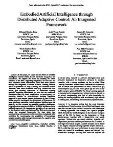
for a constant β>0. Then, the target motion q0(t) tracks the desired reference trajectory sin (βt). The cooperative adaptive control protocols of Theorem 1 were implemented at each node. As is standard in neural and adaptive control systems, reasonable positive values were initially chosen for all control and NN tuning parameters. Generally, the simulation results are not too dependent on the specific choice of parameters as long as they are selected as detailed in the Theorem and assumptions, e.g. positive. The number of NN hidden layer units can be fairly small with good performance resulting, normally in the range of 5-10. As in most control systems, however, the performance can be improved by trying a few simulation runs and adjusting the parameters to obtain good behavior. In on-line implementations, the parameters can be adjusted online to obtain better performance. 1 For NN activation function we use log-sigmoid of the form with positive slope 1 + e − kt parameter k. Number of neurons used at each node is 3. So, φm≈1 and γ≈0.04. NN gain parameter we selected as κ = 1.5 . According to (32) the pinning gain should be selected large and it was taken as c=1000. In the simulation plots we show tracking performance of positions ( q1i ) and velocities ( q2i ) for all i. At steady state all q1i and q2i are synchronized and follow the second order single link leader trajectory given by q0 and q 0 respectively. Fig. 2 shows the tracking performance of the system. One can see from the figure that positions and velocities of all the five nodes are synchronized in two different final values T which are given by the final values of [ q0 , q 0 ] . More specifically q1i ’s are synchronized with q0 and q2i ’s are synchronized with q 0 at steady state. The figure also shows the inputs ui for all agents while tracking. Fig. 3 describes the position and velocity consensus disagreement error vectors namely T T q1i − q0 , q2i − q 0 , ∀i and also the NN estimation error in terms of ⎣⎡ f i ( x ) − fˆi ( x )⎦⎤ ∀i . One can easily see that all the errors are minimized almost to zero.

(

)

Fig. 2. Tracking performance (position and velocity) and control input

48

Multi-Robot Systems, Trends and Development

Fig. 3. Disagreement vector and NN estimation error vector

Fig. 4. Comarison of f ( x ) and fˆ ( x ) Fig. 4 describes the comparison of unknown dynamics f(x) with estimated dynamics fˆ ( x ) . The figure also shows that the steady state values of f ( x ) and fˆ ( x ) are almost equal. Fig. 5 shows the NN weight dynamics. Fig. 6 is the phase plane plot of all agents, i.e. the plot of q1i ∀i (along the x -axis) and q2i ∀i (along the y − axis). At steady state the Lissajous pattern formed by all five nodes is the target node’s phase plane trajectory.

Distributed Adaptive Control for Networked Multi-Robot Systems

49

Fig. 5. NN weight dynamics

Fig. 6. Phase plane plot for all the nodes

5. Conclusion This Chapter presents a method for synchronization control for multi-agent systems of order two with unknown dynamics. It gives the design of distributed adaptive controllers for second order nonlinear systems communicating on general strongly connected digraph network structures. The agent dynamics and command generator dynamics are considered unknown. Moreover the agent dynamics need not to be same. It is shown that with the use of pinning control based on the exchange of cooperative neighborhood errors among the

50

Multi-Robot Systems, Trends and Development

agents, one can guarantee synchronization of all the robots to the single command trajectory. A simple neural network parametric approximator is introduced at each node to estimate the unknown dynamics and disturbances. The choices of control protocol as well as neural net tuning laws are selected through a Lyapunov formulation to induce synchronization within the networked multi-robot team. A Lyapunov-based proof shows the ultimate boundedness of the tracking error. Simulation results for Lagrangian agent dynamics are shown to illustrate the effectiveness of the proposed method.

6. Acknowledgements This work is supported by AFOSR grant FA9550-09-1-0278, NSF grant ECCS-0801330, and ARO grant W91NF-05-1-0314.

7. References Bo,

Yang, and Fang Huajing. 2009. Second-Order Consensus in Networks of Agents with Delayed Dynamics. Journal of Natural Sciences 14, no. 2: 158-162. Chen, F. -C, and H. K. Khalil. 1992. Adaptive control of nonlinear systems using neural networks. Int. J. Control 55, no. 6: 1299-1317. Chopra, N., and M. W. Spong. 2006. Passivity-Based Control of Multi-Agent Systems. In Advances in Robot Control, 107-134. Springer Berlin Heidelberg. Das, A., and F. L. Lewis. 2009. Distributed Adaptive Control for Synchronization of Unknown Nonlinear Networked Systems. Submitted to Automatica (December). Fax, J. Alexander, and R. M. Murray. 2004. Information Flow and Cooperative Control of Vehicle Formations. IEEE Trans. Automatic Control 49, no. 9: 1465-1476. Ge, S., and C. Wang. 2004. Adaptive neural control of uncertain MIMO nonlinear systems. IEEE Trans. Neural Networks 15, no. 3 (May): 674-692. Ge, S. S., C. C. Hang, and T. Zhang. 1998. Stable Adaptive Neural Network control. Berlin: Springer. Horn, Roger A., and Charles R. Johnson. 1994. Matrix analysis. Cambridge University Press. Hornik, K., M. Stinchombe, and H. White. 1989. Multilayer Feedforward Networks are Universal Approximations. Neural Networks 20: 359-366. Hou, Zeng-Guang, Long Cheng, and Min Tan. 2009. Decentralized robust adaptive control for the multiagent system consensus problem using neural networks. IEEE Transactions on Systems, Man, and Cybernetics, Part B 39, no. 3 (June): 636-647. Jadbabaie, Ali, Jie Lin, and S. Morse. 2003. Coordination of Groups of Mobile Autonomous Agents Using Nearest Neighbor Rules. IEEE Trans. Automatic Control 48, no. 6: 9881001. Jiang, T., and J.S. Baras. 2009. Graph algebraic interpretation of trust establishment in autonomic networks. Preprint Wiley Journal of Networks. Khalil, H. K. 1996. Nonlinear Systems. Prentice Hall. Khoo, Suiyang, Lihua Xie, and Zhihong Man. 2009. Robust Finite-Time Consensus Tracking Algorithm for Multirobot Systems. IEEE Transaction on Mechatronics 14, no. 2: 219228. Kuramoto, Yoshiki. 1975. Self-entrainment of a population of coupled non-linear oscillators. In International Symposium on Mathematical Problems in Theoretical Physics, 39:420422. Lecture Notes in Physics. Springer Berlin / Heidelberg.

Distributed Adaptive Control for Networked Multi-Robot Systems

51

Lewis, F., S. Jagannathan, and A. Yesildirek. 1999. Neural Network Control of Robot Manipulators and Nonlinear Systems. London: Taylor and Francis. Lewis, F. L., A. Yesildirek, and K. Liu. 1996. Multilayer neural net robot controller with guaranteed tracking performance. IEEE Trans. Neural Networks 7, no. 2: 388-399. Li, X., X. Wang, and G. Chen. 2004. Pinning a complex dynamical network to its equilibrium. IEEE Trans. Circuits and Systems 51, no. 10: 2074-2087. Li, Z., Z. Duan, and G. Chen. 2009. Consensus of multi-agent systems and synchronization of complex networks: a unified viewpoint. IEEE Trans. Circuits and Systems (to appear). Lu, J., and G. Chen. 2005. A time-varying complex dynamical network model and its controlled synchronization criteria. IEEE Trans. Automatic Control 50, no. 6: 841-846. Narendra, K. S. 1992. Adaptive Control of dynamical systems using neural networks. Handbook of Intelligent Control. New York: Van Nostrand Reinhold. Narendra, K. S., and K. Parthasarathy. 1990. Identification and control of dynamical systems using neural networks. IEEE Transaction of Neural Networks 1: 4-27. Olfati-Saber, R., J. A. Fax, and R. M. Murray. 2007. Consensus and cooperation in networked multi-agent systems. Proceedings of the IEEE 95, no. 1: 215-233. Olfati-Saber, R., and R. M. Murray. 2004. Consensus Problems in Networks of Agents with Switching Topology and Time-Delays. IEEE Transaction of Automatic Control 49, no. 9: 1520-1533. Polycarpou, M. M. 1996. Stable adaptive neural control scheme for nonlinear systems. IEEE Trans. Automat. Control 41, no. 3: 447-451. Qu, Z. 2009. Cooperative Control of Dynamical Systems: Applications to Autonomous Vehicles. New York: Springer-Verlag. Ren, W., and R. W. Beard. 2005. Consensus Seeking in Multiagent Systems Under Dynamically Changing Interaction Topologies. IEEE Trans. Automatic Control 50, no. 5 (May): 655-661. Ren, W., R. W. Beard. 2008. Distributed Consensus in Multi-vehicle Cooperative Control: Theory and Applications. London:Spring Verlag. Ren, W., R. W. Beard, and E. M. Atkins. 2005. A Survey of Consensus Problems in Multiagent Coordination. In Proceedings of the 2005 American Control Conference. Portland, OR, USA, June 8. Ren, W., R. W. Beard, and E. M. Atkins. 2007. Information Consensus in Multivehicle Cooperative control. IEEE Control Systems Magazine. Ren, W., K. L. Moore, and Y. Chen. 2007. High-order and model reference consensus algorithms in cooperative control of multivehicle systems. Journal of Dynamic Systems, Measurement, and Control 129: 678-688. Seo, Jin Heon, Hyungbo Shima, and Juhoon Back. 2009. Consensus of high-order linear systems using dynamic output feedback compensator: Low gain approach. Automatica 45, no. 11: 2659-2664. Spanos, D. P., R. Olfati-Saber, and R. M. Murray. 2005. Dynamic consensus on mobile networks. In 2005 IFAC World Congress. Stone, M. H. 1948. The Generalized Weierstrass Approximation Theorem. Mathematics Magazine 21, no. 4,5: 167–184,237–254.

52

Multi-Robot Systems, Trends and Development

Su, Housheng, and Xiaofan Wang. 2008. Proceedings of the 7th World Congress on Intelligent Control and Automation. In . Chongqing, China, June 25. Tsitsiklis, J. N. 1984. Problems in decentralized decision making and computation. Ph.D. dissertation, Massachusetts Institute of Technology, Cambridge, MA. Wang, X., and G. Chen. 2002. Pinning control of scale-free dynamical networks. Physica A 310, no. 3: 521-531. Yang, W., A. Bertozzi, and X. Wang. 2008. Proceedings of the 47th IEEE Conference on Decision and Control. In . Cancun, Mexico, December 9. Zhu, J., Y.P. Tian, and J. Kuang. 2009. On the general consensus protocol of multi-agent systems with double-integrator dynamics. Linear Algebra and its Applications 431: 701-715.