Hindawi Publishing Corporation Mobile Information Systems Volume 2016, Article ID 3414816, 11 pages http://dx.doi.org/10.1155/2016/3414816
Research Article Control-Scheduling Codesign Exploiting Trade-Off between Task Periods and Deadlines Hyun-Jun Cha,1 Woo-Hyuk Jeong,2 and Jong-Chan Kim1 1
Graduate School of Automotive Engineering, Kookmin University, 77 Jeongneung-ro, Seongbuk-gu, Seoul 02707, Republic of Korea Department of Computer Science, Kookmin University, 77 Jeongneung-ro, Seongbuk-gu, Seoul 02707, Republic of Korea
2
Correspondence should be addressed to Jong-Chan Kim;
[email protected] Received 1 January 2016; Revised 22 March 2016; Accepted 27 March 2016 Academic Editor: Qixin Wang Copyright © 2016 Hyun-Jun Cha et al. This is an open access article distributed under the Creative Commons Attribution License, which permits unrestricted use, distribution, and reproduction in any medium, provided the original work is properly cited. A control task’s performance heavily depends on its sampling frequency and sensing-to-actuation delay. More frequent sampling, that is, shorter period, improves the control performance. Similarly, shorter delay also has a positive effect. Moreover, schedulability is also a function of periods and deadlines. By taking into account the control performance and schedulability at the same time, this paper defines a period and deadline selection problem for fixed-priority systems. Our problem is to find the optimal periods and deadlines for given tasks that maximize the overall system performance. As our solution, this paper presents a novel heuristic algorithm that finds a high-quality suboptimal solution with very low complexity, which makes the algorithm practically applicable to large size task sets.
1. Introduction In a cyberphysical system (CPS), real-time control systems monitor and control physical systems (i.e., target plants) with precise control performance requirements and tight resource constraints. When designing such a system, two different approaches can be applied. First, the traditional approach separates the control design phase and implementation phase such that scheduling parameters such as sampling rates are determined in the control design phase without considering the scheduling issue. The second approach, known as controlscheduling codesign, takes into account both the control performance and task scheduling simultaneously for the purpose of enhancing control performance with limited resources [1– 4]. This paper advocates the second approach when designing a CPS. Performance of a real-time control system in a CPS depends on not only its functional correctness but also its scheduling parameters such as sampling frequency. With more frequent sensing and actuation, more accurate control results can be obtained [5]. Certainly, this performance enhancement is at the cost of increased computing demands. Another important but often ignored timing property is the delay between sensing and actuation, that is,
input-output delay. Since a shorter delay means more recent sensing data has been used to produce the actuation value, it can provide higher control performance [5]. Then, one interesting observation is that a task’s period, that is, inverse of sampling frequency, can be lengthened without hurting the control performance if we can somehow reduce the delay. To maintain a task’s delay within a certain range, the desired maximum delay should be used as the relative deadline in the schedulability check. If the schedulability check passes, the task’s input-output delay is guaranteed less than the relative deadline. One more timing attribute we have to discuss is jitter, which is the amount of uncertain variation of sampling time or input-output delay, called sampling jitter and inputoutput jitter, respectively. Generally, large jitter has negative effects on the control performance even though the effect is not that significant as the input-output delay [6]. Even regarding jitters, a shorter relative deadline also gives tighter upper bounds of the sampling jitter and input-output jitter such that a better control result can be produced [6]. As a result, the control performance can be enhanced by either way of shorter periods or shorter deadlines, and periods and deadlines have a trade-off relation in terms of control performance.
2
Mobile Information Systems
Besides control performance, schedulability is also heavily affected by periods and deadlines of the tasks. Generally speaking, longer periods and longer deadlines both make the system more schedulable, however, at the cost of a reduced control performance. In other words, a better control performance can be obtained with a lower chance of being schedulable. Moreover, similar to the control performance case, periods and deadlines are mutually tradable to maintain schedulability. Therefore, it is important to select proper periods and deadlines which satisfy both the control performance and the schedulability. For this control-scheduling codesign issue, an optimization problem can be formulated which finds the best feasible periods and deadlines for given tasks that maximize the overall system performance. In the literature, with a similar motivation, period selection problem has been extensively studied [7–10] for both dynamic and fixed-priority scheduling algorithms. However, period and deadline selection problem, which this paper is dealing with, has gathered relatively little attention and only the dynamic-priority case has been studied [6, 11]. With this motivation, targeting fixed-priority systems, this paper proposes a novel task set synthesis algorithm that finds the proper periods and deadlines which maximize the overall system performance while guaranteeing the system schedulability. Since, even with a small number of tasks, finding the optimal solution is intractable due to the huge solution space to be searched, our algorithm is basically structured as a search-based heuristic algorithm. As will be shown in Section 6, our algorithm has a linear complexity and finds a high-quality suboptimal solution even with a large task set. For the quantitative analysis of control performance with varying periods and deadlines, we also conduct a measurement study with an automotive control application. The measured control performance of the task is defined as a nonlinear and nonconvex function of period and deadline. This function is used as an input to our heuristic algorithm. This paper’s contribution can be summarized as follows: (i) We identify and demonstrate the trade-off relation between period and deadline in terms of control performance through actual experimental studies with an automotive control application. (ii) Exploiting the above trade-off relation, a novel task set synthesis algorithm is proposed, which heuristically finds near-optimal feasible (period and delay) combinations maximizing the overall control performance. The rest of our paper is organized as follows. The next section briefly explains related work. Section 3 presents brief background knowledge and formally describes our problem. In Section 4, the trade-off relation of control performance is formally described. Section 5 presents our heuristic algorithm for the period and deadline selection problem. The experimental results are presented in Section 6. Finally, Section 7 concludes this paper.
2. Related Work Control-scheduling codesign problem has been extensively studied in the literature. Seto et al. [7] first defined the period selection problem assuming that the control performance can be expressed as an exponential decay function of the sampling period and the tasks are scheduled using dynamicpriority methods. The problem is extended to fixed-priority systems by Seto et al. [8] by finding the finite set of feasible period ranges using a branch and bound-based integer programming method. In their work, the cost function is assumed to be a monotonically increasing function of task period. Later, Bini and Di Natale [9] proposed a faster algorithm that finds a suboptimal period assignment, which can be used for a task set of practical size that was intractable by previous methods due to its high computing demands. Recently, Du et al. [12] proposed an analytical solution using the method of Lagrange multipliers and an online algorithm for the overloaded situation. The common assumption of the above researches regarding the period selection problem is that the control performance is only affected by the sampling rate, that is, task period, of the controller. However, the delay between sensing and actuation also has a significant effect on the control performance. With this motivation, Bini and Cervin [10] incorporated each task’s sensing to actuation delay into the cost function. In their work, in order to find the optimal period assignment, cost functions are approximated as linear functions of period and delay, and the delay is also approximated assuming the fluid model scheduler. Through these approximations, they proposed an analytical solution. Wu et al. [6] further enhanced the algorithm by finding task periods and deadlines altogether for EDF scheduled systems. As a result, the problem had become a period and deadline selection problem. They showed that, by regulating relative deadlines of tasks, we can upper-limit the amount of delays and jitter each task can experience. In their work, the cost function is assumed to be a nonlinear function which increases in both period and deadline of tasks. A two-step approach was presented which first fixes periods and tries to minimize deadlines using unused resources. Recently, Tan et al. [11] proposed a new algorithm which simultaneously adjusts periods and deadlines assuming EDF scheduling and LGQ controller tasks. They showed that the new algorithm is more robust with different workloads than the previous method. Despite the above researches, however, compared to the period selection problem, the period and deadline selection problem has gained less attention even though it has more flexibility to enhance control performance with scarce resources. Moreover, only EDF scheduling is considered in the period and deadline selection problem due to its ease of schedulability analysis, though the fixed-priority scheduling is more commonly used in the practice. On the contrary, this paper is dealing with the period and deadline selection problem under the fixed-priority scheduling.
Mobile Information Systems
3 Following the notation in [6], each task’s control performance is defined as a function of its period and deadline, which is denoted by
Lateral error Lane center line
Vehicle center point
Figure 1: Lane keeping assist system. Its system error is defined as the lateral distance between the vehicle center point and the lane center line.
3. Background and Problem Description 3.1. System Model. This paper considers a system with 𝑛 independent periodic real-time tasks {𝜏1 , 𝜏2 , . . . , 𝜏𝑛 }, which control 𝑛 different plants, respectively. The tasks are scheduled by the fixed-priority scheduler and the priorities are assigned according to the Deadline Monotonic (DM) order. Each 𝜏𝑖 is characterized by the following scheduling parameters: (i) 𝐶𝑖 : the worst-case execution time (WCET). (ii) 𝑇𝑖 : the sampling period. (iii) 𝐷𝑖 : the relative deadline. From the above, 𝐶𝑖 is a known parameter decided by the control code, whereas 𝑇𝑖 and 𝐷𝑖 are operational parameters which can be controlled by system designers. Regarding deadlines, this paper considers only constrained deadlines where 𝐷𝑖 is always less than or equal to 𝑇𝑖 . During system execution, each 𝜏𝑖 generates infinite sequence of periodic jobs 𝜏𝑖,1 , 𝜏𝑖,2 , . . . with its period 𝑇𝑖 , which controls its corresponding target plant by (i) sensing the state of the plant, (ii) calculating the actuation values, and (iii) actuating the plant. 3.2. Control Performance as a Function of Period and Deadline. When defining the performance of a controller, various metrics can be used, such as transient response time and steady-state accuracy [6, 13]. In some cases, even the energy consumption can be a control performance metric [7]. Among the various control performance metrics, this paper chooses the system error as our optimization target. System error is defined as the difference between the desired state and the actual state of the plant [6]. This can be thought of as how well the plant is acting following the controller’s intention. More specifically, let us take the lane keeping assist system (LKAS) as an example. In a modern vehicle, LKAS controls the steering angle such that the vehicle is able to follow the center of its lane. Then, the system error can be defined as the lateral error between the center of the vehicle and the center of the lane, which is illustrated in Figure 1. Since this system error also varies along with time 𝑡, we further define the worst-case system error as the largest lateral error the vehicle can experience during its driving. More interested readers are referred to [14].
𝐽𝑖 (𝑇𝑖 , 𝐷𝑖 ) .
(1)
Generally, 𝐽𝑖 (𝑇𝑖 , 𝐷𝑖 ) is defined as a nonlinear cost function which increases in both 𝑇𝑖 and 𝐷𝑖 ; that is, if period or deadline increases, system error always increases. The intuition behind this assumption will be discussed in Section 4. We assume that 𝐽𝑖 (𝑇𝑖 , 𝐷𝑖 ) is not continuous but discrete in both 𝑇𝑖 and 𝐷𝑖 , which are also constrained within [𝑇𝑖min , 𝑇𝑖max ] and [𝐷𝑖min , 𝐷𝑖max ], respectively. Besides each task’s system error, the overall system error is denoted by 𝐽 (𝑇, 𝐷) ,
(2)
where 𝑇 is the vector of 𝑇𝑖 ’s and 𝐷 is the vector of 𝐷𝑖 ’s. For the notational simplicity, 𝐽(𝑇, 𝐷) is shortened to 𝐽 as in the following: 𝐽 = ∑ 𝑤𝑖 𝐽𝑖 (𝑇𝑖 , 𝐷𝑖 ) , 1≤𝑖≤𝑛
(3)
where 𝐽 is defined as a weighted sum of 𝐽𝑖 (𝑇𝑖 , 𝐷𝑖 )’s and 𝑤𝑖 is a user-defined weight constant for the purpose of normalizing each 𝐽𝑖 (𝑇𝑖 , 𝐷𝑖 ) to a desired range. Now, the system’s overall system error can be obtained by giving every task’s period and deadline. 3.3. Problem Description. Assuming the above concepts and notations, this subsection describes our period and deadline selection problem, which can be formally defined as follows. Problem Description. For a given task set {𝜏1 , 𝜏2 , . . . , 𝜏𝑛 }, each 𝜏𝑖 ’s 𝐶𝑖 and 𝐽𝑖 (𝑇𝑖 , 𝐷𝑖 ) are given a priority. Then, our problem is to find the optimal 𝑇 = (𝑇1 , 𝑇2 , . . . , 𝑇𝑛 ) and 𝐷 = (𝐷1 , 𝐷2 , . . . , 𝐷𝑛 ) such that the overall system error 𝐽(𝑇, 𝐷) is minimized while guaranteeing every 𝜏𝑖 ’s schedulability. Since it is assumed that 𝐽𝑖 (𝑇𝑖 , 𝐷𝑖 ) is not continuous, we do not try to make an analytical solution for our optimization problem. Instead, we formulate our problem as a combinatorial optimization problem. Figure 2 shows a graphical representation of an example 𝐽𝑖 (𝑇𝑖 , 𝐷𝑖 ) with 10 discrete (𝑇𝑖 , 𝐷𝑖 ) combinations. Note that since we only consider constrained deadlines, the left upper triangular matrix is not considered at all.
4. How Scheduling Affects Control Performance This section deals with the rationale behind the definition of 𝐽𝑖 (𝑇𝑖 , 𝐷𝑖 ), which is introduced in Section 3.2. It is claimed in many literatures that the control performance of a task can be defined as a function of the task period and deadline [6, 10, 11]. If the control system is composed of only a single periodic task, it should be strictly periodic and the input-output delay is simply bounded by 𝐶𝑖 . Thus, the control performance should be defined as a function of 𝑇𝑖 and 𝐶𝑖 . However, when
4
Mobile Information Systems
30
Ji (20, 20)
Ji (30, 20)
20
Ji (10, 10)
Ji (20, 10)
Ji (30, 10)
10
Ji (0, 0)
Ji (10, 0)
Ji (20, 0)
Ji (30, 0)
0
0
10
20
30
as possible without hurting the schedulability, and the job executes without any interference by higherpriority jobs once it begins. Deadline (ms)
Ji (30, 30)
Period (ms)
Figure 2: A graphical representation of an example 𝐽𝑖 (𝑇𝑖 , 𝐷𝑖 ) function with its period varying from 0 ms to 30 ms and its deadline also varying from 0 ms to 30 ms. The granularity of periods and deadlines is 10 ms.
multiple control tasks are implemented and scheduled on a shared processor, their execution is also subject to the following scheduling effects [6]: (i) Sampling Delay. Although a job is released at a certain time point, the actual beginning of the job can be delayed due to the execution of higher-priority jobs. The time distance between the release time and the actual beginning of a job is defined as a sampling delay. (ii) Input-Output Delay. The time distance between the beginning and the completion of a job is defined as an input-output delay, which is composed of the actual execution time of the job which is bounded by 𝐶𝑖 and the blocking time by higher-priority jobs. (iii) Sampling Jitter. As a task produces consecutive jobs, its sampling delay is not constant but varies according to the scheduling pattern each job experiences. The difference between the minimum and maximum sampling delay is defined as the sampling jitter of the task. (iv) Input-Output Jitter. The difference between the minimum and maximum input-output delay of a task is defined as the input-output jitter of the task. By the above scheduling effects, the actual execution of a control task is not strictly periodic and the input-output delay significantly varies due to different scheduling scenarios. Thus, the above scheduling effects as well as the control period collectively affect the control performance. Note that, for each task, the only tunable scheduling parameters are 𝑇𝑖 and 𝐷𝑖 in our system model. The control period 𝑇𝑖 itself has a significant effect on the control performance since it determines the control frequency. Besides, for the above four scheduling effects, Wu et al. [6] analyzed the worst-case scenarios as in the following under the condition that every task is schedulable: (i) Sampling delay is bounded by 𝐷𝑖 − 𝐶𝑖 , which happens when the beginning of a job is delayed as long
(ii) Input-output delay is bounded by 𝐷𝑖 , which happens when a job begins right after it is released and finishes right before the job’s deadline. (iii) Sampling jitter is bounded by 𝐷𝑖 − 𝐶𝑖 . The minimum possible sampling delay is 0 and the maximum possible sampling delay is 𝐷𝑖 − 𝐶𝑖 . Thus, the difference between the maximum and minimum sampling delay is 𝐷𝑖 − 𝐶𝑖 . (iv) Input-output jitter is bounded by 𝐷𝑖 − 𝐶𝑖𝑏 , where 𝐶𝑖𝑏 is the best-case execution time which can be simply assumed to be zero when not available. The minimum possible input-output delay is 𝐶𝑖𝑏 and the maximum possible input-output delay is 𝐷𝑖 . Thus, the difference between the maximum and minimum input-output delay is 𝐷𝑖 − 𝐶𝑖𝑏 . The analysis above shows that a shorter deadline makes shorter sampling delay and shorter input-output delay. Even the jitters can be controlled by a shorter deadline. The implication of the above analysis is that a better control performance can be obtained by shortening 𝐷𝑖 as well as 𝑇𝑖 [6]. From the above observation, we can conclude that the control performance generally increases as 𝑇𝑖 or 𝐷𝑖 decreases. In other words, 𝐽𝑖 (𝑇𝑖 , 𝐷𝑖 ), the system error, is a monotonically increasing function in both 𝑇𝑖 and 𝐷𝑖 . Note that 𝐽𝑖 (𝑇𝑖 , 𝐷𝑖 ) also reflects the effect of jitters as well as delays and sampling frequency. In order to account for the above scheduling effects when estimating the control performance, Jitterbug [15], which is a MATLAB toolbox, can be used to analyze the cost of delay and jitter in terms of control performance. Besides, TrueTime [16] provides a simulation environment which facilitates cosimulation of controller task execution and real-time scheduling. Although analysis and simulation methods are useful when estimating control performance, this paper proposes a different approach when finding 𝐽𝑖 (𝑇𝑖 , 𝐷𝑖 ). As will be further explained in Section 6.1, a measurement environment is developed for an automotive control application. In practice, 𝑇𝑖 and 𝐷𝑖 cannot be an arbitrary number but should be chosen from a number of predefined candidate parameters the software platform provides. Thus, it is practically feasible to measure the system errors for each 𝑇𝑖 and 𝐷𝑖 combination for each control task by arbitrarily making the worst-case scenarios. Using these discrete functions 𝐽𝑖 (𝑇𝑖 , 𝐷𝑖 )’s, the optimization algorithm in Section 5 can be used to find optimal 𝑇 and 𝐷 that minimize 𝐽(𝑇, 𝐷).
5. Task Set Synthesis Algorithm In order to find 𝑇 and 𝐷 with the minimum 𝐽(𝑇, 𝐷), the simplest solution is to explore the entire solution space for every (𝑇𝑖 , 𝐷𝑖 ) combination checking the schedulability and calculating the overall system error. This exhaustive search method, however, has a too high complexity such that it is not applicable to a task set even with a small number of
Mobile Information Systems
5
tasks like five or six tasks. The computational feasibility of the exhaustive search algorithm will be further discussed in Section 6.2. Instead, this section proposes an alternative heuristic algorithm that finds a suboptimal result, however, with a very low computational complexity. Even with this low complexity, our solution can find a very-high-quality solution for very large task sets, which will be shown later in Section 6.2. For the ease of explanation, let us define the following function: Schedulability (𝑇, 𝐷, 𝐶) ,
(4)
where 𝑇 and 𝐷 are vectors of chosen periods and deadlines. 𝐶 is a vector of each task’s 𝐶𝑖 ’s. It is assumed that 𝐶 is a constant vector. Inside this function, tasks are sorted according to the DM order where the task with the shortest 𝐷𝑖 gets index 1 and the task with the longest 𝐷𝑖 gets index 𝑛. Then, following Audsley et al. [17], the exact schedulability check is performed. For that, the following recursive equation computes the worst-case response time 𝑅𝑖 of each 𝜏𝑖 : 𝑅𝑖𝑘+1 = 𝐶𝑖 + ∑ ⌈ 1≤𝑚 𝑇𝑖 are not generated since we only consider constrained deadlines. The figure also depicts how our heuristic algorithm iteratively finds the solution with an example. The initial solution is set to {𝜏1 (0, 0) , 𝜏2 (0, 0) , 𝜏3 (0, 0)} ,
(7)
where each tuple is (𝑇𝑖 , 𝐷𝑖 ) pair. Then, for each iteration, the task with the lowest 𝐽𝑖 (𝑇𝑖 , 𝐷𝑖 ) is chosen and the task is moved to the proper direction as explained in Section 5. Each circled number means the movement of the consecutive search iterations. The move continues until the system becomes schedulable. In this example, after 16 moves, the final solution is found, that is, {𝜏1 (30, 30) , 𝜏2 (30, 20) , 𝜏3 (30, 20)} .
(8)
9
0.140
⑩ 0.070 0.079 ① ⑥ ⑦
0.889
0.941
0.967
0.811
0.856
0.914
0.933
0.653
0.727
0.784
0.832
0.895
0.624
0.667
0.752
0.789
0.871
0.330
0.412
0.543
0.609
0.690
0.723
0.826
0.203
0.261
0.383
0.455
0.494
0.590
0.702
0.770
0.160
0.239
0.305
0.344
0.437
0.549
0.562
0.643
0.114
0.189
0.221
0.287
0.360
0.405
0.472
0.580
0.135
0.179
0.252
0.284
0.368
0.452
0.523
40 50 60 Period (ms)
70
80
90
100
⑯ ⑭
0.000
0.039
0.050
0.092
0
10
20
30
1.000
0.240
0.959
0.980
0.897
0.918
0.942
0.722
0.833
0.892
0.929
0.690
0.719
0.803
0.852
0.879
0.515
0.559
0.629
0.754
0.786
0.838
0.352
0.427
0.492
0.617
0.656
0.707
0.812
0.255
0.325
0.439
0.505
0.605
0.667
0.742 0.637
0.137
0.173
0.196
0.311
0.335
0.401
0.546
0.580
0.056
0.086
0.110
0.183
0.236
0.285
0.371
0.412
0.475
0.583
0.000
0.034
0.073
0.096
0.122
0.156
0.213
0.272
0.384
0.463
0.525
0
10
20
30
40
50
60
70
80
90
100
②
⑨ ④
⑬
⑪
100 90 80 70 60 50 40 30 20 10 0
Period (ms)
(a) 𝜏1
(b) 𝜏2 1.000
⑮ 0.133 ⑧ ⑫ 0.052 0.096 ③ ⑤
0.954
0.992
0.887
0.929
0.979
0.791
0.857
0.900
0.947
0.665
0.728
0.810
0.871
0.909
0.501
0.622
0.685
0.744
0.825
0.842
0.347
0.463
0.523
0.565
0.671
0.758
0.773
0.288
0.356
0.446
0.536
0.580
0.635
0.716
0.174
0.204
0.286
0.391
0.436
0.486
0.614
0.696
0.150
0.159
0.245
0.315
0.374
0.422
0.479
0.592
0.184
0.231
0.000
0.036
0.064
0.084
0.116
0.215
0.257
0.322
0.400
0.559
0
10
20
30
40 50 60 Period (ms)
70
80
90
100
100 90 80 70 60 50 40 30 20 10 0
Deadline (ms)
0.508
0.988
Deadline (ms)
100 90 80 70 60 50 40 30 20 10 0
1.000 0.961
Deadline (ms)
Mobile Information Systems
(c) 𝜏3
Figure 8: The process of heuristic algorithm.
(i) Searching every possible combination of periods and deadlines checking the schedulability and overall system error. The result is optimal for the entire solution space. This approach is denoted by Exhaustive. (ii) Searching only the combinations with 𝑃𝑖 = 𝐷𝑖 , which significantly reduces the solution space compared to Exhaustive. The result is only optimal for the solution space with implicit deadlines. This approach is denoted by Implicit. (iii) Search guided by our heuristic algorithm as explained in Section 5. The result may not be optimal compared to Exhaustive. This approach is denoted by Ours. Figure 9 shows the overall system error with the above three approaches. The number of tasks is varied from 1 to 6. For each experiment, 100 task sets are generated and the result is the average of 100 task sets. As shown in the figure, Exhaustive shows the best result even though the algorithm almost never ends when the number of tasks exceeds 4. The results for 5 and 6 are approximated using a curve fitting method with quadratic equations. Comparing Implicit
3 2.5 Sum of system errors
At the final solution, 𝐽(𝑇, 𝐷) = 0.55 = 0.203 + 0.173 + 0.174. Note that when deciding the overall system error, the weights 𝑤𝑖 ’s are simply given 1 in the entire experiment. With the above exemplified task set generation method and heuristic algorithm, we compare the following three approaches:
2 1.5 1 0.5 0
1
2
3
4
5
6
Number of tasks Exhaustive Exhaustive (expected)
Implicit Ours
Figure 9: Comparison of our approach with optimal results.
and Ours, Ours wins for every six experiments. Though the difference is marginal when the number of tasks is small, note that the difference is increasing as the number of tasks increases. Table 1 shows the required computing time for the three approaches when the number of tasks varies from 1 to 10.
10
Mobile Information Systems 3
Table 1: The required computing times for the three approaches with varying number of tasks. Exhaustive 0.6835 ms 13.684 ms 1305 ms 2 min (3 hours) (12 days) (1228 days) (3 years) (30577 years) (290635 years)
Implicit 0.7885 ms 0.926 ms 6 ms 72 ms 986 ms 1100 ms (2 min) (26 min) (5 hours) (2 days)
Ours 0.69 ms 0.88 ms 0.75 ms 0.74 ms 1.65 ms 2.44 ms 16.19 ms 121 ms 609 ms 1121 ms
The numbers in parenthesis are estimated values whereas the other numbers are actually measured. From the table, Exhaustive requires more than a year when the number of tasks is only 7. Even for Implicit, when the number of tasks is 10, which is relatively small in practice, the required computing time exceeds 2 days. Therefore, we can conclude that both Exhaustive and Implicit cannot be used as practical size task sets whereas Ours finds solutions even with larger task sets. In order to prove that our heuristic algorithm produces a high-quality solution compared to other methods, we also compare Ours with the following two other heuristic algorithms: (i) At each iteration, the approach chooses the moving direction with the higher slope of 𝐽(𝑇𝑖 , 𝐷𝑖 ). This approach is denoted by Higher. (ii) At each iteration, the approach chooses the moving direction with the lower slope of 𝐽(𝑇𝑖 , 𝐷𝑖 ). This approach is denoted by Lower. Note that Ours is an extension of Lower, which additionally considers the resulting schedulability as well as the slope when deciding the moving direction. Figure 10 compares the performance of Ours with Higher and Lower. The result is the average of 100 synthesized task sets for each number of tasks from 1 to 6. As shown in the figure, Ours shows the best result compared to Higher and Lower. By comparing Higher and Lower, Lower shows a better result compared to Higher. The result first explains that taking the lower slope produces a better result than taking the higher slope. Meanwhile, Ours further enhances the performance by taking the schedulability into consideration as well as the slope at each iteration.
7. Conclusion By exploiting the trade-off relation of task periods and deadlines, this paper proposes a novel task set synthesis algorithm for maximizing the overall system performance. For conducting a measurement study regarding the control performance, a simulation environment is developed, which can easily gather the performance variations of automotive
2.5 Sum of system errors
Number of tasks 1 2 3 4 5 6 7 8 9 10
2 1.5 1 0.5 0
2
1
3 4 Number of tasks
5
6
Higher Lower Ours
Figure 10: Comparison of our approach with other heuristic methods.
control applications while applying various task periods and deadlines. Starting from the measured data, which confirms the trade-off relation, our problem is formally defined as a period and deadline selection problem. The input to our problem is each task’s WCET and its measured control performance matrix with various periods and deadlines. For the scheduling, DM fixed-priority scheduling is assumed. Since it becomes quickly intractable to find the optimal solution with even relatively small number of tasks, this paper proposes a heuristic algorithm with a linear complexity that finds a highquality suboptimal solution. Our heuristic algorithm is based on a gradient descent method with its initial solution at the smallest period and deadline for each task. Starting from the initial solution, our algorithm iteratively increases period or deadline one at a time until the task set is schedulable. For each iteration, the task and its moving direction are chosen comparing the control performance reductions. In our future work, we consider a new system configuration where multiple implicit deadline periodic tasks collectively control a single plant. For such systems, a chain of tasks actually controls a plant from sensing to actuation. By controlling each task’s sampling period, we have to indirectly control the sampling frequency and input-output delay the plant actually experiences.
Competing Interests The authors declare that there are no competing interests regarding the publication of this paper.
References ˚ en, A. Cervin, J. Eker, and L. Sha, “An introduction [1] K.-E. Arz´ to control and scheduling co-design,” in Proceedings of the 39th IEEE Confernce on Decision and Control, pp. 4865–4870, IEEE, December 2000.
Mobile Information Systems [2] F. Xia and Y. Sun, “Control-scheduling codesign: a perspective on integrated control and computing,” Dynamics of Continuous, Discrete and Impulsive Systems—Series B, vol. 13, supplement 1, pp. 1352–1358, 2006. [3] A. Cervin and J. Eker, “Control-scheduling codesign of realtime systems: the control server approach,” Journal of Embedded Computing, vol. 1, no. 2, pp. 209–224, 2005. [4] F. Xia and Y.-X. Sun, Control and Scheduling Codesign: Flexible Resource Management in Real-Time Control Systems, Springer Science & Business Media, 2008. ˚ en, [5] A. Cervin, D. Henriksson, B. Lincoln, J. Eker, and K.-E. Arz´ “How does control timing affect performance? Analysis and simulation of timing using jitterbug and truetime,” IEEE Control Systems, vol. 23, no. 3, pp. 16–30, 2003. [6] Y. Wu, G. Buttazzo, E. Bini, and A. Cervin, “Parameter selection for real-time controllers in resource-constrained systems,” IEEE Transactions on Industrial Informatics, vol. 6, no. 4, pp. 610–620, 2010. [7] D. Seto, J. P. Lehoczky, L. Sha, and K. G. Shin, “On task schedulability in real-time control systems,” in Proceedings of the 1996 17th IEEE Real-Time Systems Symposium (RTSS ’96), pp. 13–21, December 1996. [8] D. Seto, J. P. Lehoczky, and L. Sha, “Task period selection and schedulability in real-time systems,” in Proceedings of the 19th IEEE Real-Time Systems Symposium (RTSS ’98), pp. 188–198, December 1998. [9] E. Bini and M. Di Natale, “Optimal task rate selection in fixed priority systems,” in Proceedings of the 26th IEEE Real-Time Systems Symposium (RTSS ’05), 409, 399 pages, December 2005. [10] E. Bini and A. Cervin, “Delay-aware period assignment in control systems,” in Proceedings of the Real-Time Systems Symposium (RTSS ’08), pp. 291–300, December 2008. [11] L. Tan, C. Du, and Y. Dong, “Control-performance-driven period and deadline selection for cyber-physical systems,” in Proceedings of the 10th Asian Control Conference (ASCC ’15), pp. 1–6, Kota Kinabalu, Malaysia, May 2015. [12] C. Du, L. Tan, and Y. Dong, “Period selection for integrated controller tasks in cyber-physical systems,” Chinese Journal of Aeronautics, vol. 28, no. 3, pp. 894–902, 2015. [13] G. Buttazzo, M. Velasco, and P. Marti, “Quality-of-control management in overloaded real-time systems,” IEEE Transactions on Computers, vol. 56, no. 2, pp. 253–266, 2007. [14] H.-J. Cha, S.-W. Park, W.-H. Jeong, and J.-C. Kim, “Performance tradeoff between control period and delay: lane keeping assist system case study,” Journal of the Korea Society of Computer and Information, vol. 20, no. 11, pp. 39–46, 2015. [15] B. Lincoln and A. Cervin, “Jitterbug: a tool for analysis of real-time control performance,” in Proceedings of the 41st IEEE Conference on Decision and Control, vol. 2, pp. 1319–1324, IEEE, Las Vegas, Nev, USA, December 2002. ˚ en, [16] D. Henriksson, A. Cervin, M. Andersson, and K.-E. Arz´ “Truetime: simulation of networked computer control systems,” in Proceedings of the 2nd IFAC Conference on Analysis and Design of Hybrid Systems, Alghero, Italy, June 2006. [17] N. Audsley, A. Burns, M. Richardson, K. Tindell, and A. Wellings, “Applying new scheduling theory to static priority preemptive scheduling,” Software Engineering Journal, vol. 8, no. 5, pp. 284–292, 1993. [18] EVIDENCE, “Erika enterprise manual,” http://erika.tuxfamily .org/drupal/.
11 [19] B. Wymann, “Torcs manual installation and robot tutorial,” http://www.berniw.org/aboutme/publications/torcs.pdf. [20] Infineon, “Tc1797 user’s manual,” http://www.infineon.com/ cms/en/product/. [21] Tc1796 user’s manual, http://www.infineon.com/cms/en/product/. [22] National Instruments, Labview user manual, http://www.ni .com/labview/ko/. [23] PEAK-System, “Pcan-basic parameters description,” http:// www.peak-system.com/PCAN-USB.199.0.html?&L=1. [24] Logitech, Logitech g25 user manual, http://support.logitech .com/enau/product/g25-racing-wheel.
Journal of
Advances in
Industrial Engineering
Multimedia
Hindawi Publishing Corporation http://www.hindawi.com
The Scientific World Journal Volume 2014
Hindawi Publishing Corporation http://www.hindawi.com
Volume 2014
Applied Computational Intelligence and Soft Computing
International Journal of
Distributed Sensor Networks Hindawi Publishing Corporation http://www.hindawi.com
Volume 2014
Hindawi Publishing Corporation http://www.hindawi.com
Volume 2014
Hindawi Publishing Corporation http://www.hindawi.com
Volume 2014
Advances in
Fuzzy Systems Modelling & Simulation in Engineering Hindawi Publishing Corporation http://www.hindawi.com
Hindawi Publishing Corporation http://www.hindawi.com
Volume 2014
Volume 2014
Submit your manuscripts at http://www.hindawi.com
Journal of
Computer Networks and Communications
Advances in
Artificial Intelligence Hindawi Publishing Corporation http://www.hindawi.com
Hindawi Publishing Corporation http://www.hindawi.com
Volume 2014
International Journal of
Biomedical Imaging
Volume 2014
Advances in
Artificial Neural Systems
International Journal of
Computer Engineering
Computer Games Technology
Hindawi Publishing Corporation http://www.hindawi.com
Hindawi Publishing Corporation http://www.hindawi.com
Advances in
Volume 2014
Advances in
Software Engineering Volume 2014
Hindawi Publishing Corporation http://www.hindawi.com
Volume 2014
Hindawi Publishing Corporation http://www.hindawi.com
Volume 2014
Hindawi Publishing Corporation http://www.hindawi.com
Volume 2014
International Journal of
Reconfigurable Computing
Robotics Hindawi Publishing Corporation http://www.hindawi.com
Computational Intelligence and Neuroscience
Advances in
Human-Computer Interaction
Journal of
Volume 2014
Hindawi Publishing Corporation http://www.hindawi.com
Volume 2014
Hindawi Publishing Corporation http://www.hindawi.com
Journal of
Electrical and Computer Engineering Volume 2014
Hindawi Publishing Corporation http://www.hindawi.com
Volume 2014
Hindawi Publishing Corporation http://www.hindawi.com
Volume 2014