control system for an unstable process is also different from that for a ... 7th March 1997. The authors are with the Department of Chemical Engineering, National ...... 14 LUYBEN, W.L.: 'Process modelling simulation and control for chemical ...
Control-system synthesis for open-loop unstable process with time delay H.-P. Huang C.-C.Chen
Indexing terms: Open-loop unstable poles, Control-system synthesis, Time delay
Abstract: To avoid performance limitations caused by an open-loop unstable pole, a threeelement structure, which is equivalent to a twodegrees-of-freedom control design, is proposed to synthesise a control system for an open-loop unstable process with time delay. Through this proposed approach, control problems such as stabilising an unstable pole, servo-tracking and disturbance rejection can be treated independently. The resulting three-element structure can then be used to derive conventional two-degrees-of-freedom elements or conventional PID systems. Tuning rules for a PID controller are also provided. Examples are presented to illustrate the proposed method.
1
Introduction
Control system design for an open-loop unstable process is more difficult than that for a stable one. The difficulties are mostly due to the unstable nature of the dynamics, for which most design tools cannot be used. For example, the Bode stability criterion and the pole/ zero cancellation method become inapplicable when an unstable pole exists [l]. The strongly stabilising problem is also an immense obstacle for the unstable process [2]. The parity-interlacing property makes it clear that there are times when right-halfplane poles must be added in the compensator in order to stabilise the unstable process. Except for the stability problems, the performance specification which can be assigned to the control system for an unstable process is also different from that for a stable one. Some performance specifications which are very common for stable processes, however, would be impossible to achieve for unstable processes. The performance limitations due to the right-halfplane (RHP) poles and zeros in the process are discussed very early by Youla, Bongiorno and Jabr [3]. They pointed out that every RHP pole of the process is a zero of the sensitivity function of at least the same multiplicity. Freudenberg and Looze made a series of 0IEE, 1997 IEE Proceedings online no. 19971222 Paper first received 8th July 1996 and in revised form 7th March 1997 The authors are with the Department of Chemical Engineering, National Taiwan University, Taipei 10617, Taiwan, Republic of China 334
studies on performance limitations relating to RHP poles and zeros in frequency domain [4-61. Their work showed that these performance limitations are not only imposed on a specific frequency but also interfere with each other at all frequencies. These effects are important to the loop-shaping design method [7]. In this paper, such limitations in the frequency domain are found to be a lower bound of the complementary sensitivity function. Moreover, performance limitations in the time domain for time-delayed unstable processes are also discussed. These problems of performance limitations are discussed in Section 2. The objectives for controlling an open-loop unstable process should include: stabilising the unstable pole, achieving good performance in servo-tracking and in disturbance rejection. As is discussed in Section 2, the existing design methods, including those of the 2degree-of-freedom (2DF) control system, are, as usual, inadequate to achieve all these three objectives satisfactorily. Consequently, the success of a design is very much dependent on a case-by-case basis. To make up for this deficiency, a design method for the control of time-delayed unstable processes, in which the stability problem and performance problem can be taken into account separately, is thus proposed. The proposed method is conducted in a three-element structure which has three controllers. Each of these controllers has a different purpose, as mentioned above. After completion of these controllers in the three-element structure, the controllers in the conventional 2DF system are then directly derived from the three-element structure. In Section 3 , the problems of designing these three controllers in the three-element structure and the equivalence between the three-element structure and conventional 2DF structure are discussed. Since the PID controller has been considered to be the most widely used controller in industry, a PID controller tuning method evolved from the three-element structure is proposed in the paper. Although tuning of PID controllers for time-delayed unstable processes has been an active area of research
in the literature, most work has dealt only with firstorder time-delayed unstable processes. Moreover, all these studies only apply to the case where the ratio of delay to unstable time constant (i.e. 8/T) is smaller than unity [8-131. In this paper, the proposed PID method can apply to the case where 8/T is smaller than 2 for the first-order time-delayed unstable process, and is not limited to first-order unstable processes only. All the problems in tuning the PID controllers are discussed in Section 4. IEE Proc -Control Theory A p p l , Vol 144, No 4, July 1997
In Section 5 , three examples are simulated to show the performance and robustness of the proposed method. These examples include two first-order examples with 0/T < 1 and 0/T > 1, respectively. The third example is an example of a high-order process. Performance limitations
2
The existence of the RHP poles or RHP zeros in an open-loop transfer function of a process will cause some inevitable limitations on the performance of closed-loop control. Traditionally, these limitations are expressed in terms of the sensitivity function or the complementary sensitivity function [3]. Freudenberg and Looze pointed out that the existence of the RHP poles and RHP zeros would result in interactions in all frequencies [4-6]. The Bode integral relation was then extended to include processes having unstable poles in their works. In this paper, it is shown that such an integral relation will result in a lower bound of the complementary sensitivity function. Performance limitations in the time domain for time-delayed unstable processes are also discussed.
2.7
Time-domain limitation
If the process has an open-loop unstable pole, the response of the closed-loop system would inevitably go higher than the reference value in all cases. This fact can be easily understood from the following theorem. Theorem 1 Consider the unity-feedback control structure (Fig. 1). Assume that there is a RHP pole h in the process, that the corresponding feedback system is stable, and that the input signal v(t) is also stable. Then the error signal e(t) must satisfy the integral constraint e-xte(t)dt = o
(1)
For a step change in setpoint, the output of the process at the start time will fall behind the new setpoint value; therefore, the system will result in a negative error in the start. Consequently, the output of the process should rise higher than the new setpoint value to compensate these starting errors. In addition to the RHP poles, time delay in the process will also cause performance degradation in the control system. In the following, it is shown that the maximum value of the process output would be bounded from below due to the RHP pole and time delay. Corollary 2 Consider the unity-feedback control structure. Assume that there is a real RHP pole A in the process, that the corresponding feedback system is stable, and that the input signal is a unity step change in setpoint r(t). In addition, assume that there is a time delay 0 in the process. Then, the maximum value of the output ymax will be bounded from below: Ymax
2 ex'
(2)
Proof From eqn. 1, and the following relations: T ( t ) = 1,vt Y ( t )= 0, t E [O, 81 e ( t ) = 1,t E [ O ,
e]
e(t) = ~
( t-)~ ( t>)1 - Y m a x , v t
we have:
I" 1 iB
epxte(t)cit =
-
epxtcit
CO
(yma,
-
1)
e-xtdt
2
e-xtdt
Proof ymaz
=o where: S(s) is the sensitivity function, ~ ( s )is the Lapalace transform of the input signal, E(s) is the Lapalace transform of the error signal, and L(s) is the loop transfer function.
I
Fig. 1
I
Unity-Jt.edback structure
Theorem 1 shows that, if the RHP pole of the process is a real number, then any negative error in the time
domain should be compensated by the positive errors. IEE ProcContvol Theory Appl., Vol. 144, No. 4, July 1997
2 exe
Corollary 2 shows that, if the control system for a time-delayed unstable process produces no steady-state error, then the output of the process will have at least an overshoot of eaH 1. For controlling stable processes, the overshoot of the output can be suppressed arbitrarily to a desired value, for example less than 15% as usual [14]. However, as shown by Corollary 2, the magnitude of overshoot cannot be assigned arbitrarily for a time-delayed unstable process. The ability of a control system to reject disturbances will also degrade if there are RHP poles in the process. To avoid disturbance rejection, the output of the process should be kept as close to the setpoint as possible, but the minimum value of the process output is bounded from above if there are unstable poles and time delay in the process. Corollary 3 Consider the unity-feedback control structure. Assume that there is a real RHP pole h in the process, that the corresponding feedback system is stable, and that the input signal is a unity step disturbance d(t) at the output of the process. In addition, assume that there is a time delay 0 in the process. Then, the minimum value of the output y,,, will be bounded from above: Ymzn
I 1- exB
(3) 335
will satisfy the relation
where L
t
Proof We have y ( t ) = d(t) = 1, 0 < t < 8, and the following equation follows eqn. 1 immediately:
llT(.)ll00 L exe
where
IlT(.)/I w
(4)
= S Uw P IWJ) I
Proof It is obvious that
s
.rr/Z(w)
d6x(w) = 7l
-.rrl2(00)
By definition,
+ /B,(X)I 5 1 Note that the bounds proposed in corollaries 2 and 3 are very conservative. It is understood from the fact that both proposed bounds are reachable only under the assumption that an infinitely large control action is possible. This control action can only be realised by infinitely high controller gain. However, the maximum feedback gain is always limited in a time-delayed unstable process. Although the proposed bounds seems too conservative to be useful, corollaries 2 and 3 still provide us important implications on performance problems for controlling time-delayed unstable processes. First, some impossible performance specifications about overshoot can be ruled out. Secondly, as these corollaries show, in general, the performance of a control system will become worse as the product of A and 8 increases.
2.2 Frequency-domain limitation In the frequency domain, the maximum magnitude of the complementary sensitivity function of a control system TQu)is an important index for both the control performance and stability robustness. Here it is shown that the m-norm of such a TQu)has a lower bound due to the presence of the RHP pole and time delay. To do this, the following definition and theorem proposed by Freudenberg and Looze are referred to first [4]. Definition The Blaschke product for RHP zeros B,(s) is defined as:
where z,is the open-loop RHP pole, and z r i s the conjugate of zi. Theorem 4 (Freudenberg and Looze, 1985 [4]) Let h = x + iy be a RHP pole of the plant G,(s); then the complementary sensitivity function T(s),will satisfy
where O A ( u ) = tan-‘ (U - y ) / x As a complement to theorem 4, the following corollary is proposed to emphasise the lower bound of the complementary sensitivity function caused by delay and the RHP pole in the process: Corollary 5 If a plant G,(s) has a time delay 8 and a RHP pole A = x + iy, then the complementary sensitive function T(s), 336
for X = I(:
+ iy,x 2 0
+ I P 3 ) I2 1 + In IB;’(X)I 2 o Substituting this result into theorem 4,
1
n/Z(w)
--K/2(m)
In I T ( j w ) l d d x ( w ) 2 nx8
1
.-/2(a)
d~x(w) 2n x ~ In I I T ( . ) I ~ ~ --xP(m) In llT(*)llcu2 llT(-)IlmL exe The ratio of ilT(.)lmto iIT(0)ll is referred to as the peak gain ratio in most control textbooks [14, I]. For stable processes, the peak gain ratio of the control system is usually assigned to be about 1.3 [15]. However, as eqn. 4 shows, it is impossible to require the peak gain ratio to be about 1.3 for some time-delayed unstable processes. 3 Control-system synthesis in three-element structure
Although there are many studies which discuss the the issue of tuning a PID controller for a time-delayed unstable process in the unity-feedback structure [8-131, however, as shown in the preceding section, the performance improvement of the control system is limited if a unity-feedback structure is considered. Thus, the 2DF control structure should be considered to improve the performance. Nevertheless, studies on 2DF structure are still rare [16-181. In Quinn and Sanathanans’ work, the delay is approximated to a rational function by using the second-order Pade approximation [ 161. Then, a method similar to the linear algebraic method [19] is introduced to design the controllers based on the approximate model. The disadvantages of such a method are: First, it is necessary to assign a reference model of the overall system, but it is still unclear how such a reference model can be chosen which satisfies a specific performance specification for unstable processes. Moreover, the zeros of such a reference model cannot be arbitrarily assigned; thus, trial-and-error steps are needed to find an acceptable reference model. Secondly, as pointed out in the literature, such a method is applicable only for a lower ratio of time delay to unstable time constant. For larger values of such a ratio, the method is reported not to be robust for perturbation in parameters [ 181. IEE Pvoc -Control Theovy A p p l , Vol 144, No 4, July 1997
Internal model control (IMC) is a powerful method for control-system synthesis, and it is well known that the control system cannot be implemented by the IMC structure if the process is an unstable one [17]. However, as suggested by Morari and Zafiriou, one can still design the controllers using the IMC method, and then, implement the controllers in an equivalent-feedback structure. This suggestion is only true for processes without delav, but would encounter difficulties for time-delayed &table processes. The following example illustrates these difficulties. Suppose the input signal v = 11s and the process considered is
P ( s )=
Recently, Jacob and Chidambaram discussed some strategies in the design of controllers for time-delayed unstable processes in the 2DF structure [18]. However, their work was limited to the first-order process only, and because the controller in their work is assumed to be a P/PI controller, these methods are applicable only for processes in which the ratio of delay to unstable time constant is less than unity.
~
-s+p
The optimal H2 IMC controller is (-s+p){(2eep - I ) s + P } 6) = s+P
The standard IMC filter is chosen to meet the requirements of internal stability and pole-zero excess: ( T p 2Tf)S 1 f ( s )= (7-f”s 1 ) Z So, the IMC controller is
+
+
+
ds) = @ ( s ) f ( s ) -
-
(2esp- I ) s + P } { ( 7 , ” P + 2 7 - ~ ) s + I}
(-s+P){
(s
+ P)k.fs +
The equivalent feedback controller is derived from C(s) = q(s)/{1 q(s) P(s)},so we have -
After a detailed inspection on C(s), it is found that s = /3 is both the zero and pole of C(s). Because the denominator of C(s) is not in a rational form, obviously, it is not possible to cancel s = fi in C(s) explicitly. Although a controller of the form Gc(s) = X(s)/{Y(s) Z(s)e-ex} can be implemented by the structure shown in Fig. 2, however, owing to the presence of the unstable factor s = /3 in X(s), it is not admissible to execute the IMC feedback controller by such a structure [3]. Thus, to implement the IMC feedback controller for a timedelayed unstable process, it is necessary to approximate C(s) by some other method to cancel the unstable factor. Doing so unavoidably makes the design procedure very tedious. In addition to this implementation problem, another major disadvantage of using the IMC method directly is that the design of IMC filter for an unstable process is never as simple as for the stable case, and the robust-stability problem is not clearly related to the IMC filter constant as in the stable case -
Fig.3
Three-element structure for unsiuble processes
As pointed out by many studies in the literature, to control a time-delayed unstable systein is by no means a simple task [8-121. Thus, direct design of controllers in a 2DF structure is difficult for time-delayed unstable processes, because it is hard to handle stability and performance problems simultaneously. To make the relation of the design procedures to the specification requirements more transparent, a three-element control structure, as shown in Fig. 3, is thus proposed to design a 2DF system. This structure has three controllers which are designed for different objectives. Of the three controllers, C1 in the inner loop is provided to stabilise the unstable pole first. The other two controllers in the outer loop are then used to take care of servotracking and disturbance rejection by considering the inner loop as an open-loop stable process. Although there are three controllers in the proposed structure, this structure is, with one assumption which does not lose generality, equivalent to the 2-degree-of-freedom (2DF) feedback structure shown in Fig. 4. Thus, the proposed structure is used to handle the stability and performance problems independently in controller design steps, and it affords a target system from which the desired 2DF control system can be derived. This advantage makes the work of designing more straightforward and easier than designing in the conventional 2DF structure. This is discussed in detail below.
POI. G,k) =
x Is) Y(s)-Z(s)e-eS
r - - - .- - - - - - 1 II
XIS)
I
Y (SI
I I
I
I
I I
*
Fig.4
Conventional 2DF Structure I
I
I
I 1
I
I
I
I
To illustrate the equivalence of the proposed structure and the 2DF structure shown in Fig. 4, refer to Fig. 3 first. It is straightforward to derive the following relation (where d is assumed to be zero): U
IEE Proc.-Control Theory Appl., Vol. 144, No. 4, July 1997
= C1C2r - C1(l
+ C2C3)y
(5) 337
Thus, using the structure in Fig. 3 as a target, the control system in Fig. 4, which has two controllers (i.e. G,' and G,?, is constructed as:
G; = ClCZ
(6)
(7) Note that, unless C2 is semiproper (biproper), the system in Fig. 3 will not be equivalent to that in Fig. 4 completely. However, this is usually true in practice, for example in PID controllers and lead-lag controllers. If C2 is semiproper, the proposed structure can be implemented by the 2DF structure in Fig. 4, and the feedback controllers G,' and G: can be thus synthesised according to eqns. 6 and 7. 3. I Design C7 for stabilising general unstable processes The controller C1 is provided to stabilise the plant Gp so that the inner loop becomes stable. No performance issue is considered in this step for this stabilised inner loop. As the parity-interlacing property shows, we may fail to stabilise some unstable processes even without time delay, if only stable controllers are to be considered. Thus, only the following two types of timedelayed unstable processes are considered in this work:
G p ( s )=
~
Kpe--BS Ts- 1
Kpe-Bs G P ( 4 = ( T s- l)(as + 1)
(9)
For convenience, these two processes are termed the FODUP (first-order delayed unstable process) and the SODUP (second-order delayed unstable process), respectively. It is well known that a higher-order stable part of a transfer function can be approximated effectively to a stable first-order transfer function with time delay. Thus, the proposed method still can apply to the higher-order processes. It has been reported in the literature that a well tuned PIP1 controller could stabilise a FODUP if and only if BIT < 1 [21, 111. A recent study shows that this constraint will relax to B/T < 2 if the PDiPID controller is considered [22].It was also known that a SODUP could be stabilised by a well tuned P controller if and only if BIT + aIT < 1. Thus, if a PD controller is used to cancel the stable pole of a SODUP this constraint can be relaxed to BIT < 1 for a SODUP. The loop gain which stabilises a time delayed unstable process is always bounded from both below and above. The maximum loop gain KM and the minimum loop gain K, which stabilise the system can be calculated from the phase criterion of root loci. Consider the FODUP as an example. The intersections of root loci and the j w axis in the first branch (0
s
w
de) are
determined by the equation -8w
-T
+ tan-'
T w = -n
i.e. 9w = tan-' T w (10) Obviously, co = 0, which corresponds to K,, is one solution of eqn. 10. It was reported that there is one solution other than w = 0, if the value of BiT is smaller than unity [ l l , 231. The loop gain corresponding to 338
those intersections is thus determined by
K = J W (11) Numerical values of K, and KM for the FODUPs corresponding to different value of BIT(! d) are calculated out and plotted in Fig. 5. As shown in that Figure, the value of K, is independent of BIT, and the value of KM is a monotonically decreasing function of OIT. 80 -
K 40
20 0 0
0.2
0.4
6
0.6
0.8
1.0
Fig.5 K, and Ku of FODUP GJs) = exp K...
(-&)/(T5 I ) ~
KM
In this paper, C1 is chosen to be a PD controller [i.e. + l)]. Such a choice makes the proposed method applicable to BIT < 2 for a FODUP. As shown in the work of Rotstein and Lewin [9], the loop gain is an important parameter to handle the robustness issues of the control system; thus, it seems interesting to see which value of bIT(5 6) could make the feasible interval of loop gain (K,, Khf) as large as possible. For the FODUPs, the optimal value of 6 in this sense is solved for different values of BIT, and the results are plotted in Fig. 6. G,(s) = K,(bs
1.or
e Fig.6
Optimal bfov FODUP
In this work, C, is aimed at stabilising the problem; thus, C , is constructed as follows. Case (i): FODUP The value of
6 is chosen
to make the feasible interval of
(K,, K M ) largest, and the controller gain K, is chosen such that the loop gain (i.e. K,Kp) equals to i ( K , t &4).
Case (ii) : SOD UP The value of b is chosen to cancel the stable pole (i.e. b = a), and the controller gain K, is chosen such that the loop gain (i.e. K,K,) equals to i(Km + KM). In foregoing cases, the loop gain is chosen to be the mean value of K, and KM Such a choice is due to the IEE Proc -Control Theory A p p l , Vol 144, No 4, July 1997
robustness-stability consideration. For other purposes, the loop gain may be chosen by another method, for example, the optimum-gain-margin method suggested by De Paor and O'Malley [8]. The issues of robustness stability about the inner loop of the proposed three-element structure are discussed in the following two theorems. Theorem 6 Consider the open-loop transfer function
Ke-" GI "-Ts-1 Suppose that the uncertainties occur only in 8 and T, and that the closed-loop system is stable in the nominal case. Thus, the perturbed system is stable, if and only if 8 tan-' ~
r
1. So, the perturbed system is stable if and only if K < KdB17J. In the critical case,
so
If Gp and Gd, which are open-loop stable, are known, design of C, and C3 for either servotracking or disturbance rejection becomes easy and straightforward. The dynamics of Gp and GL (f GdGL) can be expressed either in nonparametric form or in parametric form. For the former, one can prepare the Bode plot of Gp and GL and read the key parameters such as bandwidth, critical gains and critical frequency accordingly. The resulting parameters can then be used to design C, and C3 for either purpose [19]. Alternatively, one can find the best approximate transfer functions of Gp and GL using the parametric-optimisation method to fit in the Bode plot, and then design controllers according to these approximate models. In this paper, controllers C, and C3 are designed by employing the IMC method according to the stable transfer function Gp and GL. The whole design process is illustrated in the following. Case (i) :FOD UP
Then the stabilising controller C1 will be
+
C,(s) = K,(bS 1) (12) where b and K,. are constructed as discussed in Section 3.1. Such a design of controller C1 will make the inner loop of Fig. 3 stable. In other words, the following equation has no RHP roots:
T S- 1 + K ( b s + l)e-'" = 0 where K = KcKp,so that
Recalling that KM is a monotonically decreasing function of BIT thus K cc KM if and only if 8 tan-'dFT -T < 4F-X Theorem 7 Consider the open-loop transfer function K(bs l)e-'" GI,(s) = T S- 1 Suppose that the uncertainty occurs only in 8, and that the closed-loop system is stable in the nominal case. Then, the closed-loop system is stable, if and only if
Gp =
K(bs + 1)e-O" T s - 1 + K(bs + l)e-'"
(13)
According to Gp,
+
[GJ = e-Os The IMC controllers q, and defined as
qb
(referring to Fig. 7) are
-T2b2/T2
Proof The proof is trivially similar to that of theorem 6. With the aid of the foregoing two theorems, the allowable parameter variations in B and T can be estimated for the proposed method, if the uncertainty does not occur in Kp. If the uncertainty in Kp occurs, theorems similar to the above two still can be derived, but the uncertainty bound on Kp should be known first.
3.2 Design of C, and C, Referring to Fig. 3, the dynamic equation of the the inner loop is
+ G:dd = Gpz+ G L = Gpz
~
where d = GLL. IEE Proc.-Control Theory Appl., Vol. 144, No. 4, July 1997
where .f, and ,fh are two standard IMC filters which serve the two degrees of freedom to shape the system for servotracking and for disturbance rejection, respectively. Then controllers C1 and C, are derived as
c, =
qa
1- q b G p
(19)
c,= q b
-
qa The controllers C2 and C3 can be implemented by the structure shown in Fig. 2. The whole system can also be implemented in the stable IMC structure or in the 2DF structure. However, in the 2DF structure, two controllers (i.e. G,' and G,? are needed instead of three in the three-element structure (i.e. C1, C, and C,). 339
Case (ii):
SODUP
Then the stabilising controller C1 will be
+
Cl(S) = K,(as 1) (21) Where K, is designed using the method described above so that the following equation has no RHP roots:
Ts - 1 where K = K,KP, so that
trol system has only one degree of freedom in design, so it is not directly compatible with a three-element system without simplification. However, as is discussed below, if some further assumptions are made, the proposed three-element design can be approximated to a PID one.
+ K e P e S= 0 GP
& = T s -Ke-eS 1+ Ke-eS
Y
Fig.8 2DF structure 11
Referring to Fig. 4, if controller G? is moved from the feedback path to the forward path, the whole system will turn into that shown in Fig. 8. In Fig. 8, the main controller in the loop should be
According to Gp,
The IMC controllers qa and q b (referring to Fig. 7) are synthesised by eqns. 17 and 18 as in the FODUP case. Thus, G,' and G: are synthesised by eqns. 6 and 7 immediately.
I
Y
GP
c
qb
Fig.7 2DF IMC structure
It is obvious that, when the process is considered to be in the nominal case, the process output in the proposed method would be
+
y = qaGPr (1 - qbGp)G:LL (26) Obviously, qa and qb are designed to improve the performance in reference tracking and disturbance rejection, respectively. Thus, the proposed method could allow the reference-tracking problem and the disturbance-rejection problem to be considered independently.
4
To simplify this 2DF control system to a 1DF PID one, further assumptions are necessary. Since, in a 1DF control system, there will be no extra degree of freedom to treat servotracking and disturbance rejection independently, the first simplification is to make the IMC filters fa and f b equal. Consequently, C, will equal unity. As a result, F and G, will be equal to C2/(1 + C,) and C1(l + C,), respectively. According to eqn. 19, C, approaches infinity in the low-frequency range so that F can be taken as unity therein. Then, if eqn. 28 is examined, it can be seen that F functions like a lowpass filter with unity gain in low-frequency range. Note that the main loop in Fig. 8 is stabilised by G, and the main concern of control signals is emphasised in thF low-frequency range. It is thus reasonable to take F as unity as the second assumption for simplification which would not endanger the stability and performance of the system. Because controller C1 is indeed a P D controller, controller G, = C1(l + C,) can be approximated to a series-form PID controller as depicted in the following. Case (i): FOD UP In this case, Cl(S) = K,(bs 1) (29)
+
Design of PID control system
There are two different forms of the ideal PID controller: the parallel form G,(s) = Kc{l + (l/tRs) + zDs>and the series form G,(s) = K,{1 + (l/zRs)>(1 + zDs). Although the parallel-form expression is more common in the literature, the series-form expression is adopted in this work for convenience in formulation. The methods of parameters interchange between these two forms are well known and can easily be found in many control textbooks [1, 241. In the following, a tuning method is developed for a PID controller from the previous three-elementstructure design. Obviously, the series-form PID con340
and the prefilter for the setpoint input is
C3(S) = 1 (31) where zf and N are the IMC filter constant and the degree of the filter, respectively. In this work, N is chosen as 2, and it can trivially be shown that C2(s)has the following properties according to this choice: lim C,(S) = 00 s-0
lim C2(s) = 0 S+oO
IEE Pro,.-Control Theory Appl., Vol. 144, No. 4, July 1997
From eqn. 34, C2(s) has just one integral mode. By making use of eqns. 32, 33 and 34, it is reasonable to approximate 1 + C2(s)with a PI controller. So G,(s) = Cl(s){l + C2(s)}= K,(I + bs){l + (l/zRs)} is approximated to a series-form PID controller. Case (ii): SODUP In this case, Cl(S) = K,(as 1) (35)
+
The simulation results for setpoint tracking and disturbance rejection are shown in Figs. 9 and 10. When the three-element system is simplified into the PID control system, a more conservative value of 1MC filter is chosen to assure robust stability. In this example, the filter constant is chosen to be 1.5, and the corresponding tuning parameters in a series PID controller are then calculated as: K, = 2.58, zR = 5.552 and ,z = 0.121. I.
2
(37)
=1
C3(S)
where 9 and N are the IMC filter constant and the degree of the filter, respectively. In this work, N is chosen as 2, and it can trivially be shown that C2(s)has the following properties according to this choice: lim Ca(s) = 00
(38)
s+o
0
0
10
5
20
15
time
Fig.9 Nominal responses
of
dgerent method~sjbr example I : setpoint
tracking
lim C z ( s ) = 0
(39)
S A 0 0
(i) proposed three-element (ii) proposed PID (iii) Rotstein et al. (iv) De Paor et al.
For similar reasons to the FODUP case, G,(s) = Cl(s){l + C2(s)] can be approximated to a PID controller. The above discussions are summarised in Table 1. Table 1: PID controller settings for FODUP and SODUP
Kpe-HS/Ts- 1
K(2Zf+ B)/K - 1
b
K,e-OS/( Ts - 1) ( a s+ 1)
K ( 2 q+ B )/K - 1
a
Note: K = KcKp
5
In this Section, three examples are simulated to check the feasibility of the proposed method. The first example is a typical FODUP for which BIT is smaller than unity. Some results in the literature for such an example are also included to compare with the proposed method. The second one is a FODUP for which 0IT is larger than unity. The third is an example of a highorder process. It is approximated to a SODUP first, and then the control system is synthesised according to this SODUP model. In all the examples, simulations in both the three-element system and PID control system are included. The integration interval is taken to be 0.005 in all simulation examples. Example 1 Consider an unstable plant as: e-0.4s ~
s-1 Referring to Fig. 6, the optimum value of 6 is 0.121 corresponding to 0IT = 0.4; thus the stabilising interval (Km,K M ) is (1, 4.17). The stabilising controller is then chosen as C,(s) = 2.58(0.121s + 1). IMC filters are chosen as fa = l/(s + 1) and fb = 140.2s + I), so the IMC controllers are s - 1 2.58(0.121s 1)e-O 4s 4a = 2.58(0.121s 1)(s 1) s - 1 2.58(0.121s l)ep0.4s qb 2.58(0.121s 1)(0.2s 1)
+
+
5
(i) proposed three-element (ii) proposed PID (iii) Rotstein et al. (iv) De Paor et al.
Simulation examples
G p ( s )=
10 15 20 time Fig. 10 Nominal responses of different methods for example 1: disturbance attenuation
0
+
+
+
+
+
+
IEE Proc -Control Theory A p p l , Val 144, No 4, July 1997
For the existing methods in the literature, Shafiei and Sehenton’s work needs to assign the closed-loop pole of the control system first, but does not address the method of choosing the proper pole [lo]. Venkatashankar and Chidambarams’ work proposed a method to tune only the PI controller, and it is obvious that its performance is inferior to that of a PID one [ll]. Huang and Lins’ method is indeed a 2DF PIDcontroller-tuning method, and the controller output of such a method is modified by a nonlinear saturation element, but it does not address how to determine the saturation range [ 121. Therefore the above-mentioned studies are not compared with the proposed method. However, the work of De Paor and O’Malley [8] and Rotstein and Lewin [9] is compared with the proposed method in this example. Tuning parameters in the PID controller of this example for these two studies and the proposed method are listed in Table 2. Note that the PID-parameter list in Table 2 is based on the parallel-form PID controller. Table 2: Different PID-controller tuning methods for example 1 Form
Kc
ZR
Depaor and O‘Malley
Parallel
1.459
2.667
0.250
Rotstein and Lewin
Parallel
2.250
5.760
0.200
This work
Parallel
2.636
5.673
0.118
ZD
34 1
As shown in Figs. 9 and 10, the overshoot of all the PID-tuning methods is over 100%. However, this fact can be understood from theorem 2. The minimum overshoot of any feedback controller will be 1= 0.492, if perfect control is possible. Because the PID controller is a low-order controller with a specific structure, the real overshoot in the control system would be much higher than that minimum value. In our experience, the overshoot would be about 2 4 times this minimum value in a PID control system. In the three-element structure, the overshoot is, indeed, suppressed, as shown in the simulation results. For comparison, the integral absolute error (IAE) corresponding to all the methods for this example are listed in Table 3. -
0 10 15 20 time Fig. 13 Robust response of three-element systems for example I : perturbation in f3
0
5
nominal case (i) positive perturbation (ii) negative perturbation
~
Table 3: IAE of example 1 for different methods Tracking
Attenuation
Depaor and O'Malley
7.855
5.789
Rotstein and Lewin
3.553
2.559
Proposed PID
3.177
2.148
Proposed three-element
1.445
0.515
olI 0
As Table 3 shows, the proposed three-element method improves the performance in both tracking and attenuation considerably according the IAE performance index. The proposed PID method is also superior to the other two methods in the sense of IAE. Although there seem to be no significant improvements in setpoint tracking when the proposed PID method is compared with Rotstein and Lewins' method, the proposed method behaves better than their method in the attenuation case. Moreover, note that the method suggested by Rotstein and Lewin is limited to 0iT < 1 for a FODUP but the proposed method can be applied to the case of 8IT < 2.
Fig. 14 tion in Kp
I
5
10 15 20 time Robust response of PID control system for example 1: perturba-
nominal case (i) positive perturbation (ii) negative perturbation
~
0
Fig. 15 tion in T
10 15 20 time Robust response of PID control system for example I : perturba5
nominal case (i) positive perturbation (ii) negative perturbation
~
ou
3r
I
10 15 20 time Fig. 11 Robust response of three-element system for example I : perturbation in K, 0
5
nominal case (i) positive perturbation (ii) negative perturbation
~
ou
I
" 1i
Fig. 16
tion in 0
Fig. 12
tI
I
0
5
342
I
I
10 15 20 time Robust response of three-element systems for example 1: pertur-
nominal case (i) positive perturbation (ii) negative perturbation
I
nominal case (i) positive perturbation (ii) negative perturbation
ol I
bation in T ~
I
10 15 20 time Robust response of PID control system for example I : perturba-
~
0.4
o.2
I
5
0
It is assumed that there are 210% parameter perturbations in Kp, T , and 0, respectively, and the foregoing design parameters are then applied to test the robustness of the proposed methods. As shown in Figs. 1116, the proposed methods are robust to parameter perturbation in this example. IEE Proc.-Control Theory Appl., Vol. 144, No. 4, July 1997
Example 2 Consider an unstable plant as
and the PID system for this example are listed in Table 4.
e-1.2s
Table 4: IAE of example 2 for different methods
G p ( s )= ___
s-1
Referring to Fig. 6, the optimum value of h is 0.524 corresponding to BIT = 1.2; thus the stabilising interval (ICm, ICM) is (1, 1.32). The stabilising controller is then chosen as Cl(s) = 1.16(0.524s + 1). The IMC filters are chosen as fa = 1/(3s + 1) and fb= 1/(1.5s + l), respectively. So, the IMC controllers would be
+ 1.16(0.524s + l)e-1.2s 1.16(0.524s+ 1)(3s+ 1) s 1 + 1.16(0.524s + l)e-1.2s qb = 1.16(0.524s + 1)(1.5s + 1) 4a =
s-1
-
The simulation results for setpoint tracking and disturbance rejection are shown in Figs. 17 and 18. When the three-element system is simplified into the PID control system, the filter constant is chosen to be 3.0, and the corresponding tuning parameters in a series PID controller are then calculated as K, = 1.16, zR = 52.20 and ,z = 0.524. To the authors' knowledge, PID-controllerdesign methods in the literature do not apply to this example [8- 121.
Tracking
Attenuation
Proposed PID
47.65
44.98
ProDosed three-element
4.29
18.72
As Table 4 shows, the proposed three-element method improves the performance in both tracking and attenuation considerably, according the IAE performance index. To test the robustness-performance issues of the proposed methods, it is assumed that there are &5% parameter perturbations in K,, T and 0, respectively. The foregoing design parameters are then introduced to test the robustness performance of the proposed methods. As shown in Figs. 19-24, the proposed methods are robust to parameter perturbation in this example.
I
0
20. 0
Fig. 17
10
20 time
30
40
Fig. 19 Robust response of three-element sy.rtem f o r example 2: perturbution in K nomqna~case (i) positive perturbation (ii) negative perturbation ~
(i) I
I
20 30 LO time Nominal responses ojdflerent methodsfor example 2: setpoint 10
tracking (i) proposed three-element (ii) proposed PID
I
01
I
20 30 LO time Fig.20 Robust response of three-element system for example 2: perturbation in T 0
10
nominal case (i) positive perturbation (ii) negative perturbation
~
I
I
I
0
10
20 time
I
30
LO
Fig. 18 Nominal responses uf djjerent methods j o r example 2: disturbance rejection (i)proposed three-element (ii) proposed PID
In tuning a PID controller for a stable process, it makes no difference whether the controller parameters are tuned in the sequence K,, zR and zD, or in the , and z ,. However, this is not true for sequence K,, Z tuning of a PID controller for an unstable process. In the proposed method, the PID controller is tuned in the sequence of K c , ,z and zR.This is why the proposed PID method still works for 1 5 B/T < 2. For the purpose of comparison, the integral absolute error (IAE) corresponding to the three-element system IEE Proc -Control Theory A p p l , Vol 144, No 4, July 1997
0
Fig.21
10
20 time
30
LO
Robust response o j three-element system for example 2: pertur-
bation in 0 nominal case (i) positive perturbation (ii) negative perturbation
~
343
The settings of the series PID controller are K, = 4.4, , Z = 2.07 and zR = 5.10 if the IMC filter constant is chosen to be 1.5. For comparison, the integral absolute error (IAE) corresponding to the three-element system and the PID system for this example (Figs. 25 and 26) are listed in Table 5.
20 30 LO time Robust response of PID control system for example 2: perturba10
0
Fig.22 tion in Kp
nominal case (i) positive perturbation (ii) negative perturbation
~
l2
Y
r
I
0
Fig.25
I
20
10
30
LO
time Nominal responses of d#erent methodsfor example 3: setpoint
tracking (i) proposed three-element (ii) proposed PID
time
Fig.23 Robust response of PID control system for example 2: perturbation in T ___ nominal case (i) positive perturbation (ii) negative perturbation
20 30 LO time Fig.26 Nominal responses of dgerent methods for example 3: disturbance rejection 10
0
12I\ I
\
(i) proposed three-element (ii) proposed PID
.U
x
-
Table 5: IAE of example 3 for different methods
_-_ I
0
Fig.24 tion in % ~
10
30
20
time Robust response of PID control system for example 2: perturba-
nominal case (i) positive perturbation (ii) negative perturbation
Example 3 Consider an unstable plant as e-o.5s
+
Tracking
LO
+
G p ( 4 = (5s - 1)(2s 1)(0.5s 1) It is well known that the stable, higher-or er part of a transfer function can be approximated ef kctively to a first-order delayed transfer function. Let us approximate this transfer function as [ 121
P
Attenuation
Proposed PID
1.16
5.37
Proposed three-element
0.72
3.04
As Table 5 shows, the proposed three-element method improves the performance in both tracking and attenuation significantly, according the IAE performance index. To test the robustness-performance issues of the proposed methods, it is assumed that there are 220% parameter perturbations in Kp, T and 8, respectively. As shown in Figs. 27-32, the proposed methods are robust to parameter perturbation in this example.
e-o.939s
+
G p ( s )c” (5s - 1)(2.07s 1) Thus the stabilising controller C,(s) is synthesised as C,(s) = 4.4(2.07s + 1). IMC filters are chosen to bef, = 142s + I) and f b = 1/(1.5s + l), respectively. The IMC controllers are then derived as 5s - I 4.4e-0.93gS qa = 4.4(2s 1)
+
qb 344
=
+
5s - 1 + 4.4e-0.939s 4.4(1.5s + 1)
time
Fig.27 Robust response of three-element system for example 3: pertur-
bation in Km ___ nom‘inal case
(i) positive perturbation (ii) negative perturbation IEE Pvoc.-Control Theory Appl., Vol. 144, No. 4,July 1997
1.2r
0
20 30 LO time Robust response of’ three-element system for example 3: prrtur10
0 Fig.28
bation in T
Fig.32 tion in 0
r
I
10
20
30
LO
time
Fig. 29 Robust response of tliree-element system for example 3: perturbation in 0 nominal case (i) positive perturbation (ii) negative perturbation
____
Fig.30 tion in Kp
20 30 CO time Robust response of PID control system for example 3: perturba10
,
nominal case (i) positive perturbation (ii) negative perturbation
~
OV Fig.31 tion in T
10
I
20 30 10 time Robust response of PID control system for example 3: perturba10
nominal case (i) positive perturbation (ii) negative perturbdon
____
IEE Proc-Control Theory Appl.. Vol. 144, No. 4, July 1997
Conclusions and discussion
Open-loop unstable processes are considered to be difficult to control in processes industries. In this paper, performance degradations for unstable processes are studied based on both the time domain and the frequency domain to highlight these difficulties which are imposed on the overshoot and the infinity norm of the complementary sensitivity function. To avoid these difficulties, a three-element structure, which is indeed a 2DF structure, is proposed to handle this problem effectively. A PID tuning method evolved from the proposed structure is also suggested. Simulation examples show a reasonable performance and robustness of the proposed method. Thus, the proposed method provide a simple and effective controller-design technique for the time-delayed unstable process. Although the performance of the proposed design method in the three-element structure is much better than that in the traditional unity-feedback structure in both tracking and attenuation, according to IAE performance index, as shown in the simulation examples, the improvement in disturbance attenuation is still not very satisfactory. To make up this deficiency, a new type of the IMC filter for qb should be considered, instead of the standard IMC filter. This is a topic for future study. The strongly stabilising conditions for the timedelayed unstable process are still unclear in the Iiterature. This means that we do not know when we must use an unstable controller to stabilise a time-delayed unstable process. Thus, the proposedl work is indeed confined to the process which can be stabilised by a PDiPID controller only. The strongly stabilising problem for the time-delayed unstable process is another challenging topic for the future. 7
0
30
~
6
0
20
time Robust response of PID control systemfor example 3: perturba-
nominal case (i) positive perturbation (ii) negative perturbation
nominal case (i) positive perturbation (ii) negative perturbation
~
0
10
References
1 KUO, B.C.: ‘Automatic control systems’ (Prentice-Hall, 1991, 6th edn.) 2 VIDYASAGAR, M.: ‘Control system synthesis-a factorization approach’ (MIT Press, 1985) 3 YOULA, D.C., BONGIORNO, J.J.J., and JABR, H.A.: ‘Modern Wiener-Hoppf design of optimal controllers - part I: The single-input-output case’, ZEEE Trans., 1976, AC-21, pp. 3-13 4 FREUDENBERG, J.S., and LOOZE, D.P.: ‘Right half plane poles and zeros and design tradeoffs in feedback system’, IEEE Trans., 1985, AC-30, pp. 555-565 5 FREUDENBERG, J.S., and LOOZE, D.P: ‘A sensitivity tradeoff for plants with time delay’, IEEE Trans., 1987, AC-32, pp. 99-104 6 LOOZE, D.P., and FREUDENBERG, J.S.: ‘Limitations of feedback properties imposed by open-loop right half plane poles’, IEEE Trans., 1991, AC-36, pp. 136-139 7 DOYLE, J.C., FRANCIS, B.A., and TANNENBAUM, A.R.: ‘Feedback control theory’ (Macmillan Publishing Co., 1992) 345
8 DE PAOR, A.M., and O’MALLEY, M.: ‘Controller of zieglernichols type for unstable process with time delay’, Int. J. Control, 1989, 49, pp. 1273-1284 9 ROTSTEIN, G.E., and LEWIN, D.R.: ‘Simple PI and PID tuning for open-loop unstable systems’, I&EC, 1991, 30, pp. 1 8 6 4 1869 10 SHAFIEI, Z., and SHENTON, T.: ‘Tuning of PID-type controller for stable and unstable systems with time delay’, Automatica, 1994, 30, pp. 1609-1615 11 VENKATAHANKAR, V., and CHIDAMBARAM, M.: ‘Design P and PI controller for unstable first-order plus time delay process’, Int. J. Control, 1994, 60, pp. 137-144 12 HUANG, C.T., and LIN, Y.S.: ‘Tuning PID controller for openloop unstable process with time delay’, Chem. Eng. Comm., 1995, 33, pp. 11-30 13 CHIDAMBARAM, M.: ‘Design of PI and PID controllers for an unstable first-order plus time delay system’, Hung. J. Ind. Chem., 1995, 23, pp. 123-127 14 LUYBEN, W.L.: ‘Process modelling simulation and control for chemical engineers’ (McGraw-Hill, 1990, 2nd edn.) 15 LUYBEN, W.L.: ‘Simple method for tuning siso controllers in multivariable systems’, Ind. Eng. Chem, Process Des. Dev., 1986, 25, pp. 654-660
346
16 SANATHANAN, C.K., and QUINN, J.S.B.: ‘Controller design for integrating and runaway processes involving time delay’, AIChE J., 1989, 35, pp. 923-930 17 MORARI, M.; and ZAFIRIOU, E.: ‘Robust process control’ (Prentice-Hall, 1989) 18 JACOB, E.F., and CHIDAMBARAM, M.: ‘Design of controllers for unstable first-order plus time delay model’, Comput. Chem. Eng., 1996, 20, ( 5 ) , pp. 579-584 19 CHEN, C.T.: ‘Control system design-conventional, algebraic and optimal method’ (Pond Woods, 1987) 20 CAMPI, M., LEE, W.S., and ANDERSON, B.D.O.: ‘Filters for internal model control design for unstable plants’. Proceedings of the 32nd conference on Decision and control, San Antonio, Texas, 1993, pp. 1343-1348 21 DE PAOR, A.M.: ‘A modified smith predictor and controller for unstable process with time delay’, Int. J. Control, 1985, 41, pp. 1025-1 036 22 HUANG, H.P., and CHEN, C.C.: ‘On stabilising a time delayed unstable process’, Chin. I. Ch. E., submitted for publication 23 HUANG, H.P., and CHEN, C.C.: ‘Control system design for openloop unstable process having time delay - a 3-block approach’. CESA ’96 IMACS Multiconference, Lille, France, July 1996, pp. 619-624 24 ASTROM. K.J., and HAGGLUND, T.: ‘PID controllers’ (Instument Society of America, 1995)
IEE Proc.-Control Theory Appl., Vol. 144, No. 4, July 1997