Feb 8, 2019 - to go to station A. By setting the train delays D1 and D2 for train 1 ... sure that both Alice and Bob reach their target station in minimum total time.
Minimal-Time Synthesis for Parametric Timed Automata? ´ Etienne Andr´e1,2,3[0000−0001−8473−9555]?? , Vincent Bloemen4? ? ? , Laure Petrucci1 , and Jaco van de Pol4,5
arXiv:1902.03013v1 [cs.LO] 8 Feb 2019
1
LIPN, CNRS UMR 7030, Universit´e Paris 13, Villetaneuse, France 2 JFLI, CNRS, Tokyo, Japan 3 National Institute of Informatics, Japan 4 University of Twente, The Netherlands 5 University of Aarhus, Denmark
Abstract. Parametric timed automata (PTA) extend timed automata by allowing parameters in clock constraints. Such a formalism is for instance useful when reasoning about unknown delays in a timed system. Using existing techniques, a user can synthesize the parameter constraints that allow the system to reach a specified goal location, regardless of how much time has passed for the internal clocks. We focus on synthesizing parameters such that not only the goal location is reached, but we also address the following questions: what is the minimal time to reach the goal location? and for which parameter values can we achieve this? We analyse the problem and present an algorithm that solves it. We also discuss and provide solutions for minimizing a specific parameter value to still reach the goal. We empirically study the performance of these algorithms on a benchmark set for PTAs and show that minimal-time reachability synthesis is more efficient to compute than the standard synthesis algorithm for reachability.
1
Introduction
Timed Automata (TA) [AD94] extend finite automata with clocks, for instance to model real-time systems. These clocks can be used to constrain transitions between two locations with a guard, e. g. the transition can only be taken if at least 5 time units have passed. Furthermore, aside from taking transitions, ?
??
???
This is the author version of the manuscript of the same name published in the proceedings of the 25th International Conference on Tools and Algorithms for the Construction and Analysis of Systems (TACAS 2019). This version contains extended definitions, and all proofs. This work is partially supported by the ANR national research program PACS (ANR-14-CE28-0002) and PHC Van Gogh project PAMPAS. Partially supported by ERATO HASUO Metamathematics for Systems Design Project (No. JPMJER1603), JST. Supported by the 3TU.BSR project.
1
x 1 = D1 x1 := 0
D’ x1 = 100 x1 := 0 Alice A x1 = D1 x1 = 100 x1 := 0 x1 := 0 A’
D
x1 = 100 x1 := 0
C’
x 1 = D1 x1 := 0 C x1 = 100 x 1 = D1 x1 := 0 Bob x1 := 0 B B’
(a) Train 1
x2 = D2 x2 := 0
D
x2 = 55 x2 := 0
D” x2 = 55 x2 := 0
B”
B
x 2 = D2 x2 := 0
(b) Train 2
Fig. 1: Train delay scheduling problem: Alice (depicted in dotted red), located at A, wants to go to station D. Bob (depicted in dashed blue), located at B, wants to go to station A. By setting the train delays D1 and D2 for train 1 and 2, make sure that both Alice and Bob reach their target station in minimum total time. it is possible to wait some time at a location. This waiting time can also be constrained by an invariant associated with the location. Multiple clocks can coexist and clocks may also be reset when taking a transition (written as x := 0 for clock x). Timed automata allow for reasoning about temporal properties of the designed system. In addition to reachability problems, it is possible to compute for TAs the minimal or maximal time required to reach a specific goal location. Such a result is valuable in practice, as it can describe the response time of a system or it may indicate when a component failure occurs. It may not always be possible to describe a real-time system with a TA. There are often uncertainties in the timing constraints, for instance how long it takes between sending and receiving a message. Optimising specific timing delays to improve the overall throughput of the system may also be considered, as shown in Example 1. Such uncertainties can however be modelled using a parametric timed automaton (PTA) [AHV93]. A PTA adds parameters, or unknown constants, to the TA formalism. By examining the reachability of a goal location, the parameters get constrained and we can observe which parameter valuations preserve the reachability of the goal location. This process, also called parameter synthesis, is definitely useful for analysing reachability properties of a system. However, this technique does disregard timing aspects to some extent. Given the parameter constraints, it is no longer possible to give clear boundaries on the time to reach the goal, as this may depend on the parameter valuations. We focus on the parameter synthesis problem while reaching the goal location in minimal time, as demonstrated in Example 1. Example 1. Consider the example in Fig. 1, which depicts a train network consisting of two trains. Both trains share locations B and D (the stations platforms) while locations A0 , B0 , C0 , D0 , B00 , and D00 represent a train travelling (tracks). The travel time for train 1 between any two stations is 100, and 55 for train 2. Train 1 stops at stations A, B, C, and D, for time D1 (and train 2 stops for D2 time units 2
at B and D). Here, the train delays D1 and D2 are parameters and x1 and x2 are clocks. Both clocks start at 0 and reset after every transition. We assume that the trains use different tracks and changing trains at the platform of a station can be done in negligible time. Alice is starting her journey from A and would like to go to D. Bob is located at B and wants to go to A. Train 1 and/or 2 can be used to travel, if both the train and the person are at the same location. Initially, both Alice and Bob wait for a train, since the initial positions of train 1 and 2 are respectively C’ and D”. We would like to set the train delays D1 and D2 in such a way that the total time for Alice and Bob to reach their target location, i. e. the PTA location for which Alice is at station D and Bob is at station A, is minimal. The optimal solution is D1 = 25 ∧ D2 = 15, which leads to a total time of 405 units1 . Note that this is neither optimal for Alice (the fastest would be D1 = 0 ∧ D2 = 5), nor optimal for Bob (D1 = 10 ∧ D2 = 0). Note that in other instances, the time to reach a goal location may be an interval, describing the lower- and upper-bound on the time. This can be achieved in the example by changing the travel time from train 1 to be between 95 and 105, by guarding the outgoing transitions from locations A0 , B0 , C0 and D0 with 95 ≤ x1 ≤ 105 (instead of x1 = 100). We focus on the lower-bound global time, meaning that we look at the minimal total time passed in the system, which may differ from the clock values as the clocks can be reset. In this paper we address the following problems: – minimal-time reachability: synthesizing a single parameter valuation for which the goal location can be reached in minimal (lower-bound) time, – minimal-time reachability synthesis: synthesizing all parameter valuations such that the time to reach the goal location is minimized, and – parameter minimization synthesis: synthesizing all parameter valuations such that a particular parameter is minimized and the goal location can still be reached (this problem can also address the minimal-time reachability synthesis problem by adding a parameter to equal with the final clock value). For all stated problems we provide algorithms to solve them and empirically compare them with a set of benchmark experiments for PTAs, obtained from [And18a]. Interestingly, compared to standard reachability and synthesis, minimal-time reachability and synthesis is in general computed faster as fewer states have to be considered in the exploration. We also look at the computability and intractability of the problems for PTAs and L/U-PTAs (PTAs for which each parameter only appears as a lower- or upper-bound). Related work. The earliest work on minimal-time reachability was by Courcoubetis and Yannakis [CY92], who first addressed the problem of computing lower 1
Alice waits for train 1 to reach A at time 225, then she hops on and exits the train on time 350 at B. There she can immediately take train 2 and reach D at time 405. Bob waits for train 2 to reach B at time 55 and takes this train. At time 125 he reaches D and can immediately hop on train 1. Bob reaches A at time 225.
3
and upper bounds in timed automata. Several algorithms have been developed since to improve performance [NTY00,ZNL16a,ZNL16b], by e. g. using parallelism. Related problems have been studied, such as minimal-time reachability for weighted timed automata [ALTP04], minimal-cost reachability in priced timed automata [BF01], and job scheduling for timed automata [AAM06]. Concerning parametric timed automata, to the best of our knowledge, the minimal-time reachability problem was not tackled in the past. The reachability-emptiness problem (“the emptiness of the parameter valuation set for which a given set of locations is reachable”) is undecidable [AHV93], with various settings considered, notably a single clock compared to parameters [Mil00] or a single rational-valued or integer-valued parameter [Mil00,BBLS15] (see [And18b] for a survey). Only severely limiting the number of clocks (e. g. [AHV93,BO14,BBLS15,AM15]), and often restricting to integer-valued parameters, can bring some decidability. Emptiness for the subclass of L/U-PTAs is also decidable [BLR05]. Minimizing a parameter can however be considered done in the setting of upper-bound PTAs (PTAs in which the clocks are only restricted from above): the exact synthesis of integer valuations for which a location is reachable can be done [BL09], and therefore the minimum valuation of a parameter can be obtained. Overview. In Section 2 we provide preliminaries on TAs and PTAs, and formalize our problem statements. Section 3 addresses the theoretical side of our problems. Section 4 addresses the parameter minimization synthesis problem. In Section 5 solve the minimal-time reachability/synthesis problems. We present our experiments in Section 6 and conclude in Section 7.
2 2.1
Preliminaries Clocks, parameters and guards
We assume a set X = {x1 , . . . , x|X| } of clocks, i. e. real-valued variables that evolve at the same rate. A clock valuation is a function νX : X → R≥0 . We write 0 for the clock valuation assigning 0 to all clocks. Given d ∈ R≥0 , νX + d denotes the valuation s.t. (νX + d)(x) = νX (x) + d, for all x ∈ X. Given R ⊆ X, we define the reset of a valuation νX , denoted by [νX ]R , as follows: [νX ]R (x) = 0 if x ∈ R, and [νX ]R (x) = νX (x) otherwise. We assume a set P = {p1 , . . . , p|P| } of parameters, i. e. unknown constants. A parameter valuation νP is a function νP : P → Q+ . We denote ./ ∈ {}, / ∈ {, ≥}. A guard g is a constraint over X ∪ P defined by a conjunction of inequalities of the form x ./ d or x ./ p, with x ∈ X, d ∈ N and p ∈ P. Given a guard g, we write νX |= νP (g) if the expression obtained by replacing each clock x ∈ C appearing in g by νX (x) and each parameter p ∈ P appearing in g by νP (p) evaluates to true. 4
2.2
Parametric timed automata
Parametric timed automata (PTA) extend timed automata with parameters within guards and invariants in place of integer constants [AHV93]. Definition 1 (PTA). A PTA A is a tuple A = (Σ, L, `0 , X, P, I, E), where: 1. 2. 3. 4. 5. 6. 7.
Σ is a finite set of actions, L is a finite set of locations, `0 ∈ L is the initial location, X is a finite set of clocks, P is a finite set of parameters, I is the invariant, assigning to every ` ∈ L a guard I(`), E is a finite set of edges e = (`, g, a, R, `0 ) where `, `0 ∈ L are the source and target locations, a ∈ Σ, R ⊆ X is a set of clocks to be reset, and g is a guard.
Given a parameter valuation νP and PTA A, we denote by νP (A) the nonparametric structure where all occurrences of a parameter p ∈ P have been replaced by νP (p). Any structure νP (A) is also a timed automaton. By assuming a rescaling of the constants (multiplying all constants in νP (A) by their least common denominator), we obtain an equivalent (integer-valued) TA, as defined in [AD94]. L/U-PTAs Definition 2 (L/U-PTA). An L/U-PTA is a PTA where the set of parameters is partitioned into lower-bound parameters and upper-bound parameters, i. e. parameters that appear in guards and invariants in inequalities of the form p / x, and of the form p .x respectively. Concrete semantics of TAs. Let us now recall the concrete semantics of TA. Definition 3 (Semantics of a TA). Given a PTA A = (Σ, L, `0 , X, P, I, E), and a parameter valuation νP , the semantics of νP (A) is given by the timed transition system (TTS) (S, s0 , →), with: |X| – S = {(`, νX ) ∈ L × R≥0 | νX |= νP (I(`))}, – s0 = (`0 , 0), – → consists of the discrete and (continuous) delay transition relations: e 1. discrete transitions: (`, νX ) 7→ (`0 , νX0 ), if (`, νX ), (`0 , νX0 ) ∈ S, and there exists e = (`, g, a, R, `0 ) ∈ E, such that νX0 = [νX ]R , and νX |= νP (g), d
2. delay transitions: (`, νX ) 7→ (`, νX + d), with d ∈ R≥0 , if ∀d0 ∈ [0, d], (`, νX + d0 ) ∈ S. (d,e)
Moreover we write (`, νX ) −→ (`0 , νX0 ) for a combination of a delay and disd
e
crete transition if ∃νX00 : (`, νX ) 7→ (`, νX00 ) 7→ (`0 , νX0 ). 5
Given a TA νP (A) with concrete semantics (S, s0 , →), we refer to the states of S as the concrete states of νP (A). A run ρ of νP (A) is a possibly infinite alternating sequence of concrete states of νP (A), and pairs of edges and delays, starting from the initial state s0 of the form s0 , (d0 , e0 ), s1 , · · · , with i = 0, 1, . . . , and di ∈ R≥0 , ei ∈ E, and (si , ei , si+1 ) ∈ →. The set of all finite runs over νP (A) is denoted by Runs(νP (A)). The P duration of a finite run ρ = s0 , (d0 , e0 ), s1 , · · · , si , is given by duration(ρ) = 0≤j≤i−1 dj . Given a state s = (`, νX ), we say that s is reachable in νP (A) if s is the last state of a run of νP (A). By extension, we say that ` is reachable; and by extension again, given a set T of locations, we say that T is reachable if there exists ` ∈ T such that ` is reachable in νP (A). The set of all finite runs of νP (A) that reach T is denoted by Reach(νP (A), T ). Minimal reachability. As the minimal time may not be an integer, but also the smallest value larger than an integer2 , we define a minimum as either a pair in Q+ × {=, >} or ∞. The comparison operators function as follows: (c, =) < ∞, (c, >) < ∞, and (c1 , �1 ) < (c2 , �2 ) iff either c1 < c2 or c1 = c2 , �1 is = and �2 is >3 . Given a set of locations T , the minimal time reachability of T in νP (A), denoted by MinTimeReach(νP (A), T ) = min{duration(ρ) | ρ ∈ Reach(νP (A), T )}, is the minimal duration over all runs of νP (A) reaching T . By extension, given a PTA, we denote by MinTimePTA(A, T ) the minimal time reachability of T over all valuations, i. e. MinTimePTA(A, T ) = minνP MinTimeReach(νP (A), T ). As we will be interested in synthesizing the valuations leading to the minimal time, let us define MinTimeSynth(A, T ) = {νP | MinTimeReach(νP (A), T ) = MinTimePTA(A, T )}. We will also be interested in minimizing the valuation of a given parameter pi (without any notion of time) reaching a given location, and we therefore define MinParamReach(A, pi , T ) = minνP {νP (pi ) | Reach(νP (A), T ) 6= ∅}. Similarly, we will be interested in synthesizing all valuations leading to the minimal valuation of pi reaching T , so let us define MinParamSynth(A, pi , T ) = {νP | Reach(νP (A), T ) 6= ∅ ∧ νP (pi ) = MinParamReach(A, pi , T )}. 2.3
Computation problems
Minimal-time reachability problem: Input: A PTA A, a subset T ⊆ L of its locations. Problem: Compute MinTimePTA(A, T )i. e. the minimal time for which T is reachable for any νP (A). 2
3
Consider a TA with a transition guarded by x > 1 from `0 to `1 , then the minimal duration of runs reaching `1 is not 1 but slightly more. When we compute the minimum over a set, we actually calculate its infimum and combine the value with either = or > to indicate if the value is present in the set.
6
Minimal-time reachability synthesis problem: Input: A PTA A, a subset T ⊆ L of its locations. Problem: Compute MinTimeSynth(A, T )i. e. set of all parameter valuations νP for which T is reachable in minimal time in νP (A). Before addressing the problems defined in Section 2.3, we will address the slightly different problem of minimal-parameter reachability, i. e. the minimization of a parameter reaching a given location (independently of time). We will see in Lemma 4 that this problem can also give an answer to the minimal-time reachability (synthesis) problem. Minimal-parameter reachability problem: Input: A PTA A, a parameter p, a subset T ⊆ L of the locations of A. Problem: Compute MinParamReach(A, T, p)i. e. the minimal valuation for p for which T is reachable for any νP (A). Minimal-parameter reachability synthesis problem: Input: A PTA A, a parameter p, a subset T ⊆ L of the locations of A. Problem: Synthesize MinParamSynth(A, T, p)i. e. set of all parameter valuations νP for which T is reachable for a minimal valuation of p in νP (A). 2.4
Symbolic semantics
Let us now recall the symbolic semantics of PTAs (see e. g. [HRSV02,ACEF09]), that we will use to solve these problems. ConstraintsP We first define P operations on constraints. A linear term over X ∪ P is of the form 1≤i≤|X| αi xi + 1≤j≤|P| βj pj +d, with xi ∈ X, pj ∈ P, and αi , βj , d ∈ Z. A constraint C (i. e. a convex polyhedron) over X ∪ P is a conjunction of inequalities of the form lt ./ 0, where lt is a linear term. ⊥ denotes the false parameter constraint, i. e. the constraint over P containing no valuation. Given a parameter valuation νP , νP (C) denotes the constraint over X obtained by replacing each parameter p in C with νP (p). Likewise, given a clock valuation νX , νX (νP (C)) denotes the expression obtained by replacing each clock x in νP (C) with νX (x). We say that νP satisfies C, denoted by νP |= C, if the set of clock valuations satisfying νP (C) is non-empty. Given a parameter valuation νP and a clock valuation νX , we denote by νX |νP the valuation over X ∪ P such that for all clocks x, νX |νP (x) = νX (x) and for all parameters p, νX |νP (p) = νP (p). We use the notation νX |νP |= C to indicate that νX (νP (C)) evaluates to true. We say that C is satisfiable if ∃νX , νP s.t. νX |νP |= C. We define the time elapsing of C, denoted by C % , as the constraint over X and P obtained from C by delaying all clocks by an arbitrary amount of time. That is, νX0 |νP |= C % iff ∃νX : X → R+ , ∃d ∈ R+ s.t. νX0 |νP |= C ∧ νX0 = νX + d. Given R ⊆ X, we define the reset of C, denoted by [C]R , as the constraint obtained from C by resetting the clocks in R, and keeping the other clocks unchanged. Given a subset P0 ⊆ P of parameters, we denote by C↓P0 the projection of C onto P0 , i. e. obtained by eliminating the clock variables and the parameters 7
in P \ P0 (e. g. using Fourier-Motzkin [Sch86]). Therefore, C↓P denotes the elimination of the clock variables only, i. e. the projection onto P. Given p, we denote by GetMin(C, p) the minimum of p in a form (c, �). Technically, GetMin can be implemented using polyhedral operations as follows: C↓{p} is computed, and then the infimum is extracted; then the operator in {=, >} is inferred depending whether C↓{p} is bounded from below using a closed or an open constraint. We extend GetMin to accommodate clocks, thus GetMin(C, x) returns the minimal clock value that x can take, while conforming to C. Symbolic semantics A symbolic state is a pair (`, C) where ` ∈ L is a location, and C its associated constraint, called parametric zone. Definition 4 (Symbolic semantics). Given a PTA A = (Σ, L, `0 , X, P, I, E), the symbolic semantics of A is defined by the labelled transition system called the parametric zone graph PZG = (E, S, s0 , ⇒), with – S = {(`, C) | C ⊆ I(`)}, � V – s0 = `0 , ( 1≤i≤|X| xi = 0)% ∧ I(`0 ) , and � – (`, C), e, (`0 , C 0 ) ∈ ⇒ if e = (`, g, a, R, `0 ) and �% C 0 = [(C ∧ g)]R ∧ I(`0 ) ∧ I(`0 ) with C 0 satisfiable. That is, in the parametric zone graph, nodes are symbolic states, and arcs are labeled by edges of the original PTA.� 0 0 Given s = (`, C), if (`, C), e, (`0 , C 0 ) ∈ ⇒, we write Succ(s, � e) = (` , C ). 0 By extension, we write Succ(s) for ∪e∈E Succ(s, e). Given s, e, s ∈ ⇒, we also e write s ⇒ s0 . d0 ,e0 d1 ,e1 Given a concrete (respectively symbolic) run (`0 , νX0 ) −→ (`1 , νX1 ) −→ dm−1 ,em−1,
e
e
em−1
0 1 ··· −→ (`m , νXm ) (respectively (`0 , C0 ) ⇒ (`1 , C1 ) ⇒ · · · ⇒ (`m , Cm )), em−1 e0 e1 we define the corresponding discrete sequence as `0 ⇒ `1 ⇒ · · · ⇒ `m . Two runs (concrete or symbolic) are said to be equivalent if their associated discrete sequences are equal. The following results (proved in, e. g. [HRSV02]) connect the concrete and the symbolic semantics.
Lemma 1. Let A be a PTA, and let ρ be a run of A reaching (`, C). Let νP be a parameter valuation. There exists an equivalent run in νP (A) iff νP |= C↓P . Proof. From [HRSV02, Propositions 3.17 and 3.18]. Lemma 2. Let A be a PTA, let νP be a parameter valuation. Let ρ be a run of νP (A) reaching (`, νX ). Then there exists an equivalent symbolic run in A reaching (`, C), with νP |= C↓P . Proof. From [HRSV02, Proposition 3.18]. 8
2.5
Reachability synthesis
Our upcoming algorithm MinParamSynth shares some similarities with the reachability-synthesis algorithm called EFSynth: this procedure takes as input a PTA A and a set of target locations T , and attempts to synthesize all parameter valuations νP for which T is reachable in νP (A). EFSynth was formalized in e. g. [JLR15] and is a procedure that may not terminate, but that computes an exact result (sound and complete) if it terminates. EFSynth traverses the parametric zone graph of A.
3
Computability and intractability
3.1
Minimal-time reachability
The following result is a consequence of a monotonicity property of L/UPTAs [HRSV02]. We can safely replace parameters with some constants in order to compute the solution to the minimal-time reachability problem, which reduces to the minimal-time reachability in a TA, which is PSPACE-complete [CY92]. Proposition 1 (minimal-time reachability for L/U-PTAs). minimal-time reachability problem for L/U-PTAs is PSPACE-complete.
The
Proof. We show that the problem reduces to the minimal-time reachability problem for TAs. Let A be an L/U-PTA. Let v0,∞ denote the valuation assigning every lower-bound parameter (resp. upper-bound parameter) in the guards of A to 0 (resp. ∞). Let A0,∞ = v0,∞ (A) denote the structure obtained as follows: any occurrence of a lower-bound parameter is replaced with 0, and any occurrence of a conjunct x / p (where p is necessarily a upper-bound parameter) is deleted, i. e. replaced with true. (x / ∞ is always satisfiable, therefore equivalent to true.) Let us show that the minimal-time reachability problem for the L/U-PTA A is equivalent to the minimal-time reachability problem for the TA A0,∞ . ⇒ Let d be the solution of the minimal-time reachability problem for A, i. e. MinTimePTA(A, T ). Let us show that T is reachable in d time units in A0,∞ . Recall that MinTimePTA(A, T ) = minνP MinTimeReach(νP (A), T ). Let νP be a4 valuation for which the minimal time is obtained. Let ρ be a run of νP (A) for which this minimal time is obtained. Let us recall the following monotonicity result for L/U-PTAs. Basically, any run of a valuation is also a run of a “larger” valuation (i. e. smaller lowerbound parameters and larger upper-bound parameters). Lemma 3 ([HRSV02]). Let A be an L/U-PTA and νP be a parameter valuation. Let νP0 be a valuation such that for each upper-bound parameter p+ , νP0 (p+ ) ≥ νP (p+ ) and for each lower-bound parameter p− , νP0 (p− ) ≤ νP (p− ). Then any run of νP (A) is a run of νP0 (A). 4
This valuation is not necessarily unique.
9
Therefore, ρ is a run of A0,∞ , and therefore T is reachable in d time units in A0,∞ . ⇐ Let d be the solution of the minimal-time reachability problem for A0,∞ , i. e. MinTimeReach(A0,∞ , T ), and let us show there exists a parameter valuation νP such that T is reachable in d time units in νP (A). Let ρ be a run of A0,∞ for which T is reachable in d time units. The result could follow immediately from Lemma 3—if only assigning 0 and ∞ to parameters was a proper parameter valuation. From [HRSV02,BL09], if a location is reachable in the TA obtained by valuating lower-bound parameters with 0 and upper-bound parameters with ∞, then there exists a sufficiently large constant C such that this run exists in νP (A) such that νP assigns 0 to lower-bound and C to upper-bound parameters. Here, we can trivially pick d, as any clock constraint x ≤ d will be satisfied for a run of duration d. Let νP assign 0 to lower-bound and d to upper-bound parameters. Then, ρ is a run of νP (A). Therefore, T is reachable in d time units in νP (A), which concludes the proof. The result finally follows from the fact that minimal-time reachability problem for TAs is PSPACE-complete [CY92]. t u Computing the minimal time for which a location is reached (Proposition 1) does not mean that we are able to compute exactly all valuations for which this location is reachable in minimal time. In fact, we show that it is not possible in a formalism for which the emptiness of the intersection is decidable—which notably rules out its representation as a finite union of polyhedra. The proof idea is that representing it in such a formalism would contradict the undecidability of the emptiness problem for (normal) PTAs. Proposition 2 (intractability of minimal-time reachability synthesis for L/U-PTAs). The solution to the minimal-time reachability synthesis problem for L/U-PTAs cannot be represented in a formalism for which the emptiness of the intersection is decidable. Proof (by reductio ad absurdum). We use a reasoning sharing similarities with [BL09,JLR15] and with Propositions 3 and 5. Assume the solution to the minimal-time reachability synthesis problem for L/U-PTAs can be represented in a formalism for which the emptiness of the intersection is decidable. Assume an arbitrary PTA A with an initial location `0 ; assume a given target location `f . Add a new clock x not used in A (and never reset); add a new upper-bound parameter pu . Augment A as follows: add a new initial location `00 , and a transition guarded with x = 0 from `00 to `0 . Add a transition guarded by x = 2∧x < pu from `00 to a new location `0f . Add a transition guarded by x ≤ 1 from `f to `0f . Make `f urgent5 . The construction is given in Fig. 2. Also, turn A into an L/UPTA as in the proof of Proposition 5: for any parameter p0 , any guard of the 5
An urgent location is a location where time cannot elapse (depicted in dotted yellow in our figures, and which can be encoded using an extra clock).
10
`00
x=0
`0
A
`f
x≤1
x = 2 ∧ x < pu `0f
Fig. 2: Intractability of minimal-parameter reachability synthesis for L/U-PTAs. form x / p0 , x .p0 , x = p0 with x / p0u , x .p0l , p0l ≤ x ≤ p0u , respectively. The obtained PTA A0 made of the parameters set {p0l , p0u | p0 ∈ P} ∪ {pu } is an L/U-PTA. Clearly, `0f is reachable in A0 in time 2 by taking the transition from `00 to `0f , for any valuation νP such that νP (pu ) > 2. In addition, it is reachable in A0 in time ≤ 1 for all valuations of pu iff there exists a parameter valuation for which `f is reachable in A in ≤ 1 time unit. Now, assume the solution to the minimal-time reachability synthesis problem for L/U-PTAs can be represented in a formalism for which the emptiness of the intersection is decidable. Let K be this solution in A0 for T = {`0f }. Then, there exists a parameterVvaluation reaching `f in A in time ≤ 1 iff the intersection of K with pu < 2 ∧ i pli = pui is non-empty. But since reachability emptiness is undecidable for PTAs over bounded time (typically in ≤ 1 time unit) [ALM18, Theorem 17], this leads to a contradiction. Therefore, K cannot be represented in a formalism for which the emptiness of the intersection is decidable. t u
3.2
Minimal-parameter reachability
For the full class of PTAs, we will see that these problems are clearly out of reach: if it was possible to compute the solution to the minimal-parameter reachability or minimal-parameter reachability synthesis problem, then it would be possible to answer the reachability emptiness problem—which is undecidable in most settings [And18b]. We first show that an algorithm for the minimal-parameter synthesis problem can be used to solve the minimal-time synthesis problem, i. e. the minimalparameter synthesis problem is harder than the minimal-time synthesis problem. Lemma 4 (minimal-time from minimal-parameter synthesis). An algorithm that solves the minimal-parameter synthesis problem can be used to solve the minimal-time synthesis problem by extending the PTA. Proof. Assume we are given an arbitrary PTA A, a set of target locations T , and a global clock xglobal that never resets. We construct the PTA A0 from A by adding a new parameter pglobal , and for every edge (`, g, a, R, `0 ) in A0 such that `0 ∈ T , we replace g by g∧xglobal = pglobal . Note that when a target location from T is reached, we have that xglobal = pglobal , hence by minimizing pglobal we also 11
`00
x=0
`0
`f
A
x := 0
`00f x=0∧x=p
x=1∧x=p
`0f
Fig. 3: Intractability of minimal-parameter reachability for PTAs minimize xglobal . Thus, by solving MinParamSynth(A0 , T, pglobal ), we effectively solve MinTimeSynth(A, T ). The following result states that synthesis of the minimal-value of the parameter is intractable for PTAs. Proposition 3 (intractability of minimal-parameter reachability for PTAs). The solution to the minimal-parameter reachability for PTAs cannot be computed in general. Proof (by reductio ad absurdum). Assume the solution to the minimalparameter reachability for PTAs can be computed. Assume an arbitrary PTA A with an initial location `0 ; assume a given target location `f . Add a new clock x and a new parameter p not used in A. Augment A as follows: add a new initial location `00 , and a transition guarded with x = 0 from `00 to `0 . Add an unguarded transition from `f to a new location `00f resetting x, and then a transition guarded by x = 0 ∧ x = p from `00f to a new location `0f . Add an unguarded transition from `00 to `0f guarded with x = 1∧x = p. Let A0 denote this augmented PTA. The construction is given in Fig. 3. Clearly, `0f is reachable in A0 if p = 1. In addition, it is reachable in A0 for p = 0 iff there exists a parameter valuation for which `f is reachable in A. Now, assume the solution to the minimal-parameter reachability for A0 and p can be computed. Let K denote this solution (which will typically be p = 0 or p = 1 depending on whether `f is reachable in A). Then, there exists a parameter valuation reaching `f in A iff K is equal to p = 0. But since reachability emptiness is undecidable for PTAs [AHV93], this leads to a contradiction. Therefore, K cannot be computed in general. t u The intractability of minimal-parameter reachability synthesis for PTAs will be implied by the upcoming Proposition 5 in a more restricted setting. Still, we prove it below with a slightly different condition from Proposition 5. Proposition 4 (intractability of minimal-parameter reachability synthesis for PTAs). The solution to the minimal-parameter reachability synthesis for PTAs cannot be represented in a formalism for which the emptiness of the intersection is decidable. 12
Proof (by reductio ad absurdum). Assume the solution to the minimalparameter reachability synthesis for PTAs can be represented in a formalism for which the emptiness of the intersection is decidable. We use a reasoning similar to that of the proof of Proposition 3. Assume an arbitrary PTA A, and augment it into A0 as in Fig. 3. Again, `0f is reachable in A0 if p = 1. In addition, it is reachable in A0 for p = 0 iff there exists a parameter valuation for which `f is reachable in A. Now, assume the solution to the minimal-parameter reachability synthesis for A0 and p can be represented in a formalism for which the emptiness of the intersection is decidable. Let K denote this solution: note that this solution will either be p = 1 (with all other parameters unconstrained) if `f is unreachable in A, or a constraint of the form p = 0 ∧ K 0 , for some constraint K 0 over the other parameters. Then, there exists a parameter valuation reaching `f in A iff K ∧ p = 0 is not empty. But since reachability emptiness is undecidable for PTAs [AHV93], this leads to a contradiction. Therefore, K cannot be represented in a formalism for which the emptiness of the intersection is decidable. t u Let us now address two subclasses for which the reachability-emptiness problem is decidable: the class of L/U-PTAs (Section 3.2), and the class of 1-clock PTAs (Section 4.3). Intractability of the synthesis for L/U-PTAs. The following result states that synthesis is intractable for L/U-PTAs. In particular, this rules out the possibility to represent the result using a finite union of polyhedra. Proposition 5 (intractability of minimal-parameter reachability synthesis for L/U-PTAs). The solution to the minimal-parameter reachability synthesis for L/U-PTAs cannot always be represented in a formalism for which the emptiness of the intersection is decidable and for which the minimization of a variable is computable. Proof. From Lemma 4 and Proposition 2.
t u
The minimal-parameter reachability problem remains open for L/U-PTAs (see Section 7). Despite these negative results, we will define procedures that address not only the class of L/U-PTAs, but in fact the class of full PTAs. Of course, these procedures are not guaranteed to terminate.
4 4.1
Minimal parameter reachability synthesis The algorithm
We give MinParamSynth(A, T, p) in Algorithm 1. It maintains a set W of waiting symbolic states, a set P of passed states, a current optimum Opt and the associated optimal valuations K. While W is not empty, a state is picked in line 6. If it is a target state (i. e. ` ∈ T ) then the projection of its constraint 13
onto p is computed, and the minimum is inferred (line 10). If that projection improves the known optimum, then the associated parameter valuations K are completely replaced by the one obtained from the current state (i. e. the projection of C onto P). Otherwise, if C↓{p} is equal to the known optimum (line 14), then we add (using disjunction) the associated valuations. Finally, if the current state is not a target state and has not been visited before, then we compute its successors and add them to W in lines 17 and 18. Note that if W is implemented as a FIFO list with “pick” the first element, then this algorithm is a classical BFS procedure. Also note that if we replace lines 10-15 with the statement K ← K ∨C↓P (i. e. adding the parameter valuations to K every time the algorithm reaches a target location), we obtain the standard synthesis algorithm EFSynth from e. g. [JLR15], that synthesizes all parameter valuations for which a set of locations is reachable.
Algorithm 1: MinParamSynth(A, T, p) input output 1 2 3 4 5 6 7 8 9 10 11 12 13 14 15 16 17
18
19
: A PTA A with symbolic initial state s0 = (`0 , C0 ), a set of target locations T , a parameter p. : Constraint K over the parameters solution of MinParamSynth(A, T, p).
// Initialization W ← {s0 } P←∅ Opt ← ∞ K←⊥ // Main loop while W 6= ∅ do Pick s = (`, C) from W W ← W \ {s} P ← P ∪ {s} if ` ∈ T then sopt ← GetMin(C, p) if sopt < Opt then Opt ← sopt K ← C↓P else if sopt = Opt then K ← K ∨ C↓P else
// waiting set // passed set // current optimum // current optimum valuations
// s is a target state // compute local optimum // the optimum is strictly better // we found a new best optimum: replace it // completely replace the found valuations // the optimum is equal to the one known // add the found valuations
// otherwise explore successors for each s0 ∈ Succ(s) do // add to waiting list only if not seen before if s0 ∈ / W ∧ s0 ∈ / P then W ← W ∪ {s0 }
return K
Example 2. Consider the PTA A in Fig. 4, and run MinParamSynth(A, {`3 }, p1 ). The initial state is s1 = (`1 , x ≥ 0) (we omit the trivial constraints pi ≥ 0). Its successors s2 = (`3 , x ≥ 2∧p1 > 2) and s3 = (`2 , x ≥ 0∧p2 > 1) are added to W. Pick s2 from W: it is a target, and therefore GetMin(C2 , p1 ) is computed, which gives (2, >). Since (2, >) < ∞, we found a new minimum, and K becomes C2 ↓P , i. e. p1 > 2. Pick s3 from W: it is not a target, therefore we compute its successors s4 = (`3 , x ≥ 2 ∧ p1 = 2 ∧ 1 < p2 < 2) and s5 = (`3 , x ≥ 2 ∧ p1 = p3 = 2 ∧ p2 > 1). Pick s4 : it is a target, with GetMin(C4 , p1 ) = (2, =). As (2, =) < (2, >), we found 14
x < p1 ∧x=2
`3
x < p2 ∧x=1 `1
x = p1 ∧x=2 ∧ x > p2
x = p1 ∧x=2 ∧ x = p3 `2
x := 0
Fig. 4: PTA exemplifying Algorithm 1. a new minimum, and K is replaced with C4 ↓P , i. e. p1 = 2 ∧ 1 < p2 < 2. Pick s5 : it is a target, with GetMin(C4 , p1 ) = (2, =). As (2, =) = (2, =), we found an equally good minimum, and K is improved with C5 ↓P , giving a new K equal to (p1 = 2 ∧ 1 < p2 < 2) ∨ (p1 = p3 = 2 ∧ p2 > 1). As W = ∅, K is returned. 4.2
Correctness
Proposition 6 (soundness). Assume MinParamSynth(A, T, p) terminates with result K. Let νP |= K. Then νP |= MinParamSynth(A, T, p). Proof. Recall that MinParamSynth(A, pi , T ) = {νP | Reach(νP (A), T ) 6= ∅ ∧ νP (pi ) = MinParamReach(A, pi , T )}. Let us first show that Reach(νP (A), T ) 6= ∅, i. e. that T is reachable in νP (A). From Algorithm 1 (lines 13 and 15), K is only made of the projection onto P of constraints associated with target symbolic states (i. e. such that ` ∈ T ). Therefore, from Lemma 1 there exists an equivalent concrete run reaching T in νP (A), which gives that Reach(νP (A), T ) 6= ∅. Let us now show that νP (pi ) = MinParamReach(A, pi , T ). First, notice that the entire parametric zone graph of A is explored by Algorithm 1, except when branches are cut (i. e. successors are not explored), i. e. when a target state is met: in that case, the state is added to P (line 8) but its successors are not computed. Let us show that this result in no loss of information for MinParamSynth (in fact, the same holds for EFSynth, see e. g. [JLR15]). The following result (proved in e. g. [HRSV02,JLR15]) states that the successor of a symbolic state can only restrict the parameter constraint. Lemma 5. Let (`0 , C 0 ) ∈ Succ((`, C)). Then C 0 ↓P ⊆ C↓P . From Lemma 5, the unexplored symbolic states do not add any valuation to the known valuation in K. In addition, as Algorithm 1 iteratively searches for the minimal Opt, then 1. Opt is eventually the minimum of p, and 2. K contains all associated parameter valuations associated with p. Therefore, νP (pi ) = MinParamReach(A, pi , T ).
t u
Proposition 7 (completeness). Assume MinParamSynth(A, T, p) terminates with result K. Let νP |= MinParamSynth(A, T, p). Then νP |= K. 15
Proof. Recall that MinParamSynth(A, pi , T ) = {νP | Reach(νP (A), T ) 6= ∅ ∧ νP (pi ) = MinParamReach(A, pi , T )}. We use a reasoning dual to Proposition 6. By definition of MinParamReach, νP is the smallest one for which T is reachable. Since ∃` ∈ T reachable in νP (A), from Lemma 2, there exists an equivalent symbolic run in A reaching (`, C), with νP |= C↓P . In addition, from the way the minimum is managed in Algorithm 1 together with the fact that the unexplored states do not bring any interesting valuation (Lemma 5), then this symbolic state (`, C) is kept by Algorithm 1, either at line 13 or line 15, and no further symbolic state will replace it. Thus, C↓P ⊆ K, and therefore νP |= K. t u Theorem 1 (correctness). Assume MinParamSynth(A, T, p) terminates with result K. Assume νP . Then νP |= K iff νP |= MinParamSynth(A, T, p). t u
Proof. From Propositions 6 and 7. 4.3
A subclass for which the solution can be computed
We show that synthesis can effectively be achieved for PTAs with a single clock, a decidable subclass. Proposition 8 (synthesis for one-clock PTAs). The solution to the minimal-parameter reachability synthesis can be computed for 1-clock PTAs using a finite union of polyhedra. Proof. Let us prove termination of Algorithm 1. In [AM15], we showed that the parametric zone graph of a 1-clock PTA is finite. By computing successors of symbolic states, Algorithm 1 clearly explores (a subpart of) the parametric zone graph of A. In addition, no symbolic state is explored twice, thanks to the P set. Therefore, Algorithm 1 terminates for 1-clock PTA and returns a finite union of polyhedra (from the way K is synthesized). The correctness follows from Theorem 1. t u
5
Minimal time reachability synthesis
For minimal-time reachability and synthesis, we assume that the PTA contains a global clock xglobal that is never reset. Otherwise, we extend the PTA by simply adding a ‘dummy’ clock xglobal without any associated guards or invariants. 5.1
The algorithm
We give MinTimeSynth(A, T, p) in Algorithm 2. We maintain a priority queue Q of waiting symbolic states and order these by their minimal time (for the initial state this is 0). We further maintain a set P of passed states, a current time optimum Topt (initially ∞), and the associated optimal valuations K. We first explain the synthesis algorithm and then the reachability variant. 16
Algorithm 2: MinTimeSynth(A, T, xglobal ) input output 1 2 3 4 5 6 7 8 9 10 11 12 13 14 15 16 17
: A PTA A with symbolic initial state s0 = (`0 , C0 ), a set of target locations T , a global clock that never resets xglobal . : Minimal time Topt constraint K over the parameters.
// Initialization Q ← {(0, s0 )} P←∅ K←⊥ Topt ← ∞ // Main loop while Q 6= ∅ do (t, s = (`, C)) = Q.Pop() P ← P ∪ {s} if t > Topt then break else if ` ∈ T then K ← K ∨ (C ∧ xglobal = t)↓P
// take head of the queue and remove it // when s is a target state and t ≤ Topt // valuations for which t = Topt
else for each s0 ∈ Succ(s) do if s0 ∈ Q ∨ s0 ∈ P then continue t0 ← GetMin(s0 .C, xglobal ) if t0 ≤ Topt then if s0 .` ∈ T ∧ t0 < Topt then Topt ← t0 Q.Push((t0 , s0 ))
18
19
// priority queue ordered by time // passed set // current optimum parameter valuations // current optimum time
// otherwise explore successors // ignore seen states // get minimal time of s0 .C // only add states not exceeding Topt // new lower time to target // add to the priority queue
return (Topt , K)
Minimal-time reachability synthesis. While Q is not empty, the state with the lowest associated minimal time t is popped from the head of the queue (line 6). If this time t is larger than Topt (line 8), then this also holds for all remaining states in Q. Also all successor states from s (or successors of any state from Q) cannot have a better minimal time, thus we can end the algorithm. Otherwise, if s is a target state, we assume that t ≮ Topt and thus t = Topt (we guarantee this property when pushing states to the queue). Before adding the parameter valuations to K in line 10, we intersect the constraint with xglobal = t in case the clock value depends on parameters, e. g. if C is xglobal = p.6 If s is not a target state, then we consider its successors in lines 12-18. We ignore states that have been visited before (line 13), and compute the minimal time of s0 in line 14. We compare t0 with Topt in line 15. All successor states for which t0 exceeds Topt are ignored, as they cannot improve the result. If s0 is a target state and t0 < Topt , then we update Topt . Finally, the successor state is pushed to the priority queue in line 18. Note that we preserve the property that t ≮ Topt for the states in Q. Minimal-time reachability. When we are interested in just a single parameter valuation, we may end the algorithm early. The algorithm can be terminated as soon as it reaches line 10. We can assert at this point that Topt will not decrease 6
In case t is of the form (c, >) with c ∈ Q+ , then the intersection of C with the linear term xglobal = t would result in ⊥, as the exact value t is not part of the constraint. In the implementation, we intersect C with xglobal = t + ε, for a small ε > 0.
17
any further, since all remaining unexplored states have a minimal time that is larger than or equal to Topt . 5.2
Correctness
Algorithm 2 is a semi-algorithm; if it terminates with result (Topt , K), then K is a solution for the MinTimeSynth problem. Correctness follows from the fact that the algorithm explores exactly all symbolic states in the parametric zone graph that can be reached in at most Topt time, except for successors of target states. Note (again) that successors of a symbolic state can only restrict the parameter constraint. Furthermore, Topt is checked and updated for every encountered successor to ensure that the first time a target state is popped from the priority queue Q, it is reached in Topt time (after which Topt never changes).
6
Experiments
We implemented all our algorithms in the IMITATOR tool [AFKS12] and compared their performance with the standard (non-minimization) EFSynth parameter synthesis algorithm from [JLR15]. For the experiments, we are interested in analysing the performance (in the form of computation time) of each algorithm, and comparing that with the performance of standard synthesis. Benchmark models. We collected PTA models and properties from the IMITATOR benchmarks library [And18a] which contains numerous benchmark models from scientific and industrial domains. We selected all models with reachability properties and extended these to include: (1) a new clock variable that represents the global time xglobal , i. e. a clock that does not reset, and (2) a new parameter pglobal along with the linear term xglobal = pglobal for every transition that targets a goal location, to ensure that when minimizing pglobal we effectively minimize xglobal . In total we have 68 models, and for every experiment we used the extended model that includes both the global time clock xglobal and the corresponding parameter pglobal . Subsumption. For each algorithm that we consider, it is possible to reduce the search space with the following two reduction techniques: – State inclusion [DT98]: Given two symbolic states s1 = (`1 , C1 ) and s2 = (`2 , C2 ) with `1 = `2 , we say that s1 is included in s2 if all parameter valuations for s1 are also contained in s2 , e. g. C1 is p > 5 and C2 is p > 2. We may then conclude that s1 is redundant and can be ignored. This check can be performed in the successor computation (Succ) to remove included states, without altering correctness for minimal-time (or parameter) synthesis. – State merging [AFS13]: Two states s1 = (`1 , C1 ) and s2 = (`2 , C2 ) can be merged if `1 = `2 and C1 ∪ C2 is a convex polyhedron. The resulting state (`1 , C1 ∪ C2 ) replaces s1 and s2 and is an over-approximation of both states. However, reachable locations, minimality, and executable actions are preserved. 18
State inclusion is a relatively inexpensive computational task and preliminary results showed that it caused the algorithm to perform equally fast or faster than without the check. Checking for merging is however a computationally expensive procedure and thus should not be performed for every newly found state. For all BFS-based algorithms (standard synthesis and minimal-parameter synthesis) we merge every BFS layer. For the minimal-time synthesis algorithm, we empirically studied various merging heuristics and found that merging every ten iterations of the algorithm yielded the best results. We assume that both the inclusion and merging state-space reductions are used in all experiments (all computation times include the overhead the reductions), unless otherwise mentioned. Run configurations. For the experiments we used the following configurations: – MTReach: Minimal-time reachability, – MTSynth: Minimal-time synthesis, – MTSynth-noRed: Minimal time synthesis, without reductions, – MPReach: Minimal-parameter reachability (of pglobal ), and – MPSynth: Minimal-parameter synthesis (of pglobal ), and – EFSynth: Classical reachability synthesis. R Coretm i7Experimental setup. We performed all our experiments on an Intel 4710MQ processor with 2.50GHz and 7.4GiB memory, using a single thread. The six run configurations were executed on each benchmark model, with a timeout of 3600 seconds. All our models, results, and information on how to reproduce the results are available on https://github.com/utwente-fmt/OptTime-TACAS19.
Results. The results of our experiments are displayed in Fig. 5. MTSynth vs EFSynth. We observe that for most of the models MTSynth clearly outperforms EFSynth. This is to be expected since all states that take more than the minimal time can be ignored. Note that the experiments that appear on a vertical line between 0.1s < x < 1s are a scaled-up variant of the same model, indicating that this scaling does not affect minimal-time synthesis. Finally, the model plotted at (1346, 52) does not heavily modify the clocks. As a consequence, MTSynth has to explore most of the state space while continuously having to extract the time constraints, making it inefficient. MPSynth vs EFSynth. We can see that MPSynth performs more similar to EFSynth than MTSynth, which is to be expected as the algorithms differ less. Still, MPSynth significantly outperforms EFSynth. This is also because fewer states have to be explored to guarantee optimality (once a parameter exceeds the minimal value, all its successors can be ignored). MTSynth vs MPSynth. Here, we find that MTSynth outperforms MPSynth, similar to the comparison with EFSynth. The results also show a second scalable model around (0.003, 10) and we see that MPSynth is able to solve the ‘bad performing model’ for MTSynth as quickly as EFSynth. Still, we can conclude that the minimal-time synthesis problem is in general more efficiently solved with the MTSynth algorithm. 19
1 0.1
0.01 10
100
1000
10 1 0.1
0.01 0.001 0.01
0.1
1
10
100
Time MTSynth (sec)
1000
Time MPSynth (sec)
(25% timeout)
100 10 1 0.1
0.01 0.001 0.01
0.1
1
10
100
Time MTReach (sec)
0.001 0.01
1000
1
10
100
1000 (40% timeout)
100 10 1 0.1
0.01 0.001
0.001 0.01
0.1
1
10
100
Time MTSynth (sec)
1000 (25% timeout)
1000 100 10 1 0.1
0.01 0.001
(9% timeout)
0.1
Time MPSynth (sec)
1000
(25% timeout)
1000
0.001
1 0.1
(25% timeout)
100
0.001
10
0.01
(38% timeout)
1
Time MTSynth (sec)
100
0.001
Time MTSynth−noRed (sec)
0.1
1000 (40% timeout)
Time MPSynth (sec)
0.001 0.01
1000 (62% timeout)
10
0.001
Time MTSynth (sec)
Time EFSynth (sec)
100
(40% timeout)
(62% timeout)
Time EFSynth (sec)
1000
0.001 0.01
0.1
1
10
100
1000
Time MPReach (sec) (34% timeout)
Fig. 5: Scatterplot comparisons of different algorithm configurations. The marks on the red dashed line did not finish computing within the allowed time (3600s).
MTSynth vs MTSynth-noRed. Here we can see the advantage of using the inclusion and merging reductions to reduce the search space. For most models there is a non-existent to slight improvement, but for others it makes a large difference. While there is some computational overhead in performing these reductions, this overhead is not significant enough to outweigh their benefits. MTReach vs MTSynth. With MTReach we expect faster execution times as the algorithm terminates once a parameter valuation is found. The experiments show that this is indeed the case (mostly visible from the timeout line). However, we also observe that for quite a few models the difference is not as significant, implying that synthesis results can often be quickly obtained once a single minimal-time valuation is found. MPReach vs MPSynth. Here we also expect MPReach to be faster than its synthesis variant. While it does quickly solve six instances for which MPSynth timed out, other than that there is no real performance gain. We also argue here that synthesis is obtained quickly when a minimal parameter bound is found. 20
Of course we are effectively computing a minimal global time, so results may change when a different parameter is minimized.
7
Conclusion
We have designed and implemented several algorithms to solve the minimal-time parameter synthesis and related problems for PTAs. From our experiments we observed in general that minimal-time reachability synthesis is in fact faster to compute compared to standard synthesis. We further show that synthesis while minimizing a parameter is also more efficient, and that existing search space reductions apply well to our algorithms. Aside from the performance improvement, we deem minimal-time reachability synthesis to be useful in practice. It allows for evaluating which parameter valuations guarantee that the goal is reached in minimal time. We consider it particularly valuable when reasoning about real-time systems. On the theoretical side, we did not address the minimal-parameter reachability problem for L/U-PTAs (we only showed intractability of the synthesis). While finding the minimal valuation of a given lower-bound parameter is trivial (the answer is 0 iff the target location is reachable), finding the minimum of an upper-bound parameter boils down to reachability-synthesis for U-PTAs, a problem that remains open in general (it is only solvable for integer-valued parameters [BL09]), as well as to shrinking timed automata [SBM14], but with 0-coefficients in the shrinking vector—not allowed in [SBM14]. A direction for future work is to improve performance by exploiting parallelism. Parallel random search could significantly speed up the computation process, as demonstrated for timed automata [ZNL16b,ZNL16a]. Another interesting research direction is to look at maximizing the time to reach the target, or to minimize the upper-bound time to reach the target (e. g. for minimizing the worst-case response-time in real-time systems); a preliminary study suggests that the latter problem is significantly more complex than the minimal-time synthesis problem. One may also study other quantitative criteria, e. g. minimizing cost parameters.
References AAM06. Yasmina Abdedda¨ım, Eugene Asarin, and Oded Maler. Scheduling with timed automata. Theoretical Computer Science, 354(2):272–300, 2006. ´ ACEF09. Etienne Andr´e, Thomas Chatain, Emmanuelle Encrenaz, and Laurent Fribourg. An inverse method for parametric timed automata. International Journal of Foundations of Computer Science, 20(5):819–836, 2009. AD94. Rajeev Alur and David L. Dill. A theory of timed automata. Theoretical Computer Science, 126(2):183–235, 1994. ´ AFKS12. Etienne Andr´e, Laurent Fribourg, Ulrich K¨ uhne, and Romain Soulat. IMITATOR 2.5: A tool for analyzing robustness in scheduling problems. In FM, volume 7436 of Lecture Notes in Computer Science, pages 33–36. Springer, 2012.
21
AFS13.
AHV93. ALM18.
ALTP04.
AM15.
And18a.
And18b.
BBLS15.
BF01.
BL09.
BLR05.
BO14.
CY92.
DT98.
HRSV02.
´ Etienne Andr´e, Laurent Fribourg, and Romain Soulat. Merge and conquer: State merging in parametric timed automata. In ATVA, volume 8172 of Lecture Notes in Computer Science, pages 381–396. Springer, 2013. Rajeev Alur, Thomas A. Henzinger, and Moshe Y. Vardi. Parametric realtime reasoning. In STOC, pages 592–601, New York, NY, USA, 1993. ACM. ´ Etienne Andr´e, Didier Lime, and Nicolas Markey. Language preservation problems in parametric timed automata. http://arxiv.org/abs/1807. 07091, 2018. Rajeev Alur, Salvatore La Torre, and George J. Pappas. Optimal paths in weighted timed automata. Theoretical Computer Science, 318(3):297–322, 2004. ´ Etienne Andr´e and Nicolas Markey. Language preservation problems in parametric timed automata. In FORMATS, volume 9268 of Lecture Notes in Computer Science, pages 27–43. Springer, 2015. ´ Etienne Andr´e. A benchmark library for parametric timed model checking. ¨ In Cyrille Artho and Peter Csaba Olveczky, editors, FTSCS, volume 1008 of Communications in Computer and Information Science. Springer, 2018. To appear. ´ Etienne Andr´e. What’s decidable about parametric timed automata? International Journal on Software Tools for Technology Transfer, 2018. To appear. Nikola Beneˇs, Peter Bezdˇek, Kim Gulstrand Larsen, and Jiˇr´ı Srba. Language emptiness of continuous-time parametric timed automata. In ICALP, Part II, volume 9135 of Lecture Notes in Computer Science, pages 69–81. Springer, 2015. Gerd Behrmann and Ansgar Fehnker. Efficient guiding towards costoptimality in UPPAAL. In TACAS, volume 2031 of Lecture Notes in Computer Science, pages 174–188. Springer, 2001. Laura Bozzelli and Salvatore La Torre. Decision problems for lower/upper bound parametric timed automata. Formal Methods in System Design, 35(2):121–151, 2009. Gerd Behrmann, Kim Guldstrand Larsen, and Jacob Illum Rasmussen. Optimal scheduling using priced timed automata. SIGMETRICS Perform. Eval. Rev., 32(4):34–40, 2005. Daniel Bundala and Jo¨el Ouaknine. Advances in parametric real-time reasoning. In Mathematical Foundations of Computer Science 2014 - 39th International Symposium, MFCS 2014, Budapest, Hungary, August 25-29, 2014. Proceedings, Part I, volume 8634 of Lecture Notes in Computer Science, pages 123–134. Springer, 2014. Costas Courcoubetis and Mihalis Yannakakis. Minimum and maximum delay problems in real-time systems. Formal Methods in System Design, 1(4):385–415, 1992. Conrado Daws and Stavros Tripakis. Model checking of real-time reachability properties using abstractions. In Bernhard Steffen, editor, TACAS, volume 1384 of Lecture Notes in Computer Science, pages 313–329. Springer, 1998. Thomas Hune, Judi Romijn, Mari¨elle Stoelinga, and Frits W. Vaandrager. Linear parametric model checking of timed automata. Journal of Logic and Algebraic Programming, 52-53:183–220, 2002.
22
JLR15.
Aleksandra Jovanovi´c, Didier Lime, and Olivier H. Roux. Integer parameter synthesis for timed automata. IEEE Transactions on Software Engineering, 41(5):445–461, 2015. Mil00. Joseph S. Miller. Decidability and complexity results for timed automata and semi-linear hybrid automata. In HSCC, volume 1790 of Lecture Notes in Computer Science, pages 296–309. Springer, 2000. NTY00. Peter Niebert, Stavros Tripakis, and Sergio Yovine. Minimum-time reachability for timed automata. In IEEE Mediteranean Control Conference, 2000. SBM14. Ocan Sankur, Patricia Bouyer, and Nicolas Markey. Shrinking timed automata. Information and Computation, 234:107–132, 2014. Sch86. Alexander Schrijver. Theory of linear and integer programming. John Wiley & Sons, Inc., New York, NY, USA, 1986. ZNL16a. Zhengkui Zhang, Brian Nielsen, and Kim Guldstrand Larsen. Distributed algorithms for time optimal reachability analysis. In FORMATS, volume 9884 of Lecture Notes in Computer Science, pages 157–173. Springer, 2016. ZNL16b. Zhengkui Zhang, Brian Nielsen, and Kim Guldstrand Larsen. Time optimal reachability analysis using swarm verification. In SAC, pages 1634–1640. ACM, 2016.
23