Controlled Experiments to Derive Walking Behaviour



&RQWUROOHG([SHULPHQWVWR'HULYH:DONLQJ%HKDYLRXU

Winnie Daamen and Serge Hoogendoorn Faculty of Civil Engineering and Geosciences Delft University of Technology Delft The Netherlands EJTIR, , no. 1 (2003), pp. 39 - 59 5HFHLYHG0DUFK $FFHSWHG0D\ 7RDVVHVVWKHGHVLJQRIZDONLQJLQIUDVWUXFWXUHVXFKDVWUDQVIHUVWDWLRQVVKRSSLQJPDOOVVSRUW VWDGLXPVHWFDVZHOODVWRVXSSRUWSODQQLQJRIWLPHWDEOHVIRUSXEOLFWUDQVLWWRROVWRDLGWKH GHVLJQHUDUHQHHGHG7RWKLVHQGPLFURVFRSLFDQGPDFURVFRSLFSHGHVWULDQIORZPRGHOVFDQ DQGKDYHEHHQDSSOLHG7RFDOLEUDWHDQGYDOLGDWHVXFKPRGHOVDVZHOODVWRJDLQPRUHLQVLJKW LQWR WKH FKDUDFWHULVWLFV RI SHGHVWULDQ IORZV XQGHU D YDULHW\ RI FLUFXPVWDQFHV YHU\ GHWDLOHG SHGHVWULDQ IORZ GDWD DUH UHTXLUHG 7KLV LV ZK\ 'HOIW 8QLYHUVLW\ RI7HFKQRORJ\KDVUHFHQWO\ FDUULHGRXWH[SHULPHQWDOSHGHVWULDQIORZUHVHDUFK 7KLV SDSHU GHVFULEHV WKH H[SHULPHQWDO GHVLJQ GHWHUPLQDWLRQ RI SURFHVV YDULDEOHV PHDVXUHPHQW VHWXS HWF  WKH UHVXOWLQJ PLFURVFRSLF SHGHVWULDQ GDWD DV ZHOO DV VRPH ILUVW UHVXOWV IRU WKH QDUURZ ERWWOHQHFN H[SHULPHQW %RWK PLFURVFRSLF DQG PDFURVFRSLF FKDUDFWHULVWLFVRISHGHVWULDQIORZVDUHSUHVHQWHG,QWHUHVWLQJILUVWUHVXOWVSHUWDLQWRWKHZD\ LQ ZKLFK WKH QDUURZ ERWWOHQHFN LV XVHG XQGHU VDWXUDWHG IORZ FRQGLWLRQV DQGWKHXVHRIWKH VSDFHRUUDWKHUZLGWK XSVWUHDPRIWKHERWWOHQHFNLQFDVHRIFRQJHVWLRQ

,QWURGXFWLRQ The traditional way of designing transfer stations is based on rules of thumb. These rules convey experience concerning the behaviour of passengers in transfer stations. However, they only consider static situations. Furthermore, a scientific foundation for these rules has yet to be provided. Similar arguments hold for the planning of timetables, which involves approximating the time people actually need to transfer. Different types of passengers, such as elderly people and parents with children, need different transfer times. Adopting accurately estimated transfer times will both remove excessive waiting times from a timetable as well as reduce the probability for passengers to miss their connection, thereby increasing the traveller’s comfort and the timetable’s reliability.

40

&RQWUROOHG([SHULPHQWVWR'HULYH:DONLQJ%HKDYLRXU

To support the design and planning process, Delft University of Technology, in co-operation with Holland Railconsult, has developed the simulation model SimPed to estimate both mean and variability of walking times incurred by transferring passengers and to visualise walking patterns inside transfer stations and other pedestrian areas (Daamen, 2002). Also, the microscopic simulation model NOMAD has been developed, which predicts pedestrian behaviour in general walking facilities using microscopic behavioural rules (Hoogendoorn and Bovy, 2002). Before these models can be applied, they need to be calibrated and validated. This can be achieved by comparing model results with empirical data. However, little data on pedestrian behaviour exist and most of these data sets have been gathered in Asia (Japan, Hong Kong (Lam, Morral and Ho, 1992)). However, pedestrian characteristics in Asia differ significantly from those of Western European pedestrians (for example length and width of the pedestrians, as well as cultural differences). Furthermore, the data are generally macroscopic, meaning that they describe the characteristics of the flow rather than of the individual pedestrians. Although these data may be adequate to roughly validate the model, they will generally not suffice to calibrate the model parameters or to test the underlying theoretical hypotheses of walking behaviour. Therefore, new data sets need to be gathered for the validation of the software tools. Preferably, data are collected in stations (for that is one of the specific application areas of SimPed), but the required approval has been refused because of privacy matters. Among the disadvantages of gathering data in railway stations are the expected problems in the automatic tracking of pedestrians. Because of the low ceilings, video cameras cannot be placed in ideal positions (right above the pedestrian flows) in order to collect exact locations of pedestrians. On top of these technical problems, the data will contain traffic conditions that occur under specific non-controllable circumstances. As a result, whether the data will include all situations that are deemed relevant is highly unlikely. If we are for instance interested in observing crossing flows, where the composition of the two directions is 50-50%, the probability that this situation will occur and last for a considerable period of time is very slim. To overcome these problems, the Transportation and Traffic Engineering Section of Delft University of Technology has performed unique experimental research by organising walking behaviour experiments. The advantage of performing experiments is the total control of the circumstances and the flexibility to vary each of the influencing variables one by one to see effects of these variables on the behaviour of the individual pedestrians and of the total pedestrian flow. From the gathered video data both macroscopic and microscopic relations can be derived. For more information on the transformation of video data to information, we refer to Hoogendoorn and Daamen (2002). This paper describes the performed experiments and the first macroscopic results from the research. First, we give a short overview of the state of the art of pedestrian observations. Then, we formulate the research objectives and we derive the experiments to be carried out. After a short report of the day of the experiments itself, we show some preliminary results, we got from one of the experiments. Finally, we end with some conclusions.



:LQQLH'DDPHQDQG6HUJH+RRJHQGRRUQ

41

6WDWHRIWKHDUWRIHPSLULFDOUHVHDUFKRQSHGHVWULDQEHKDYLRXU This section presents a very brief (and therefore non-exhaustive) overview of some of the empirical facts regarding pedestrian walking behaviour and flow characteristics. These facts concern among other things the relation between walking speed and energy consumption, the factors influencing walking speeds, and the use of space by pedestrians. Other important features of pedestrian flows are discussed, such as self-organisation, and co-operation between pedestrians. 0DFURVFRSLFIORZFKDUDFWHULVWLFV Several authors have considered macroscopic pedestrian flow properties empirically. For instance, recent work of Lam and Cheung (2000) investigate collective walking behaviour for different types of pedestrian facilities (commercial areas, shopping areas, etc.) in Hong Kong and compare results (eg. walking speeds) to other countries. Speed-density-flow models developed for Hong Kong are similar to those developed for Singapore for similar facilities (Lam, Morrall and Ho, 1992). However, no single model fits all pedestrian facilities, indicating that more data collection is required for a larger range of flow conditions. Other studies are due to Navin and Wheeler (1969), Older (1968), Pushkarev and Zupan (1975), and Weidmann (1993). For sake of illustration, Weidmann (1993) presented the following relation between walking speed and density for one-directional flow 1 1  −1.913 − N N  9H (N ) = 1.34 1 − H  

   MDP 

   

(1)

where N is the density in P/m2, and where N DP denotes the jam-density of 5.4 P/m2. The free 0 P/m2)equals 1.34 speed of the pedestrians with different purposes of walking (where N m/s. Shopping pedestrians have a free speed of 1.04 m/s, commuters of 1.45 and the free speed for tourists is 0.99 m/s (Weidmann, 1993). Clearly, eqn. (1) can be used to determine the relation between the density and equilibrium flow as well. M

:DONLQJVSHHGVDQGVSDWLDOXVH Different factors affect the walking speeds of pedestrians, such as the SHUVRQDOFKDUDFWHULVWLFV RI SHGHVWULDQV (age, gender, size, health, etc.), FKDUDFWHULVWLFV RI WKH WULS (walking purpose, route familiarity, luggage, trip length), SURSHUWLHV RI WKH LQIUDVWUXFWXUH (type, grade, attractiveness of environment, shelter), and finally HQYLURQPHQWDO FKDUDFWHULVWLFV (ambient, and weather conditions). Besides the exogenous factors, the walking speed also depends on the pedestrian density. At some traffic condition beyond free flow, pedestrians are limited in forward movement by people to the front and side. Weidmann (1993) provides a comprehensive overview of the most important studies. With respect to the pedestrian’s spatial use, both ‘lateral spatial use’ and ‘longitudinal spatial use’ are important. For one, pedestrians will generally not be able to walk in a straight line; the required walkway width theoretically depends on the walking speed. These deviations are however rather small (i.e. approximately 5 cm). Pedestrians will also need more space in the longitudinal direction with increasing walking speeds. This is in part caused by the additional

&RQWUROOHG([SHULPHQWVWR'HULYH:DONLQJ%HKDYLRXU

42

space needed to take a step. Empirical studies have shown that the relation between the longitudinal space used and the speed is given by the following relation $(9 ) = $

MDP

 9 − 0.52 ln  1 −  9 

I

  

(2)

where 9 is the walking speed, 9I is the average free walking speed (9I ≈ 1.34 m/s), $= /: denotes the required area (i.e. longitudinal spatial use / multiplied by the lateral spatial use :), and $MDP is the largest area for which walking is impossible ($MDP ≈ 0.19 m2). Note this relation implicitly defines the speed density relation presented in (Weidmann, 1993). &ROOHFWLYHEHKDYLRXUDQGVHOIRUJDQLVDWLRQ It is well known that in pedestrian crowds, flows of pedestrians walking in opposing directions tend to separate. This common phenomenon will be referred to as G\QDPLF ODQH IRUPDWLRQ or VWUHDPLQJ (Older, 1968). The formation of lanes is the main reason for the relative small loss of capacity in case of bi-directional pedestrian flows (in the range of 4% to 14.5% (Weidmann, 1993). It is interesting to note that the structure of the lanes that are formed are equal for countries where traffic regulations are left-hand or right-hand based: it turns out that for walkways of moderate width, the lanes are formed on the right-hand side. Similar results have been established for crossing flows (Toshiyuki, 1993), albeit in the form of strips or moving clusters composed of pedestrians walking in the same direction. :DONLQJEHKDYLRXUDQGLQWHUDFWLRQ Goffman (1971) describes how the environment of the pedestrian is observed through a mostly subconscious process called VFDQQLQJ in order to side-step small obstructions on the flooring. Golson and Dabbs (1974) observe that women spend more time scanning the sidewalk than men. Wolff (1973) argues that a KLJK GHJUHH RI FRRSHUDWLRQ EHWZHHQ SHGHVWULDQV is an intrinsic part of pedestrian behaviour, without which walking would be impossible: pedestrians expect others to be co-operative rather than obstructive in the completion of their walking tasks. Goffman’s notion of scanning the infrastructure is also applicable to describe the interaction with other pedestrians. He describes how pedestrians assume that the pedestrians, who are in a small closed circle around him, are those pedestrians that he must check up on. Pedestrians who are a person or two away are neglected. The scanning area is not a circle, but an ellipse, which is narrow to either side of the individual and longest in front of him. Moreover, the area of the ellipse changes constantly according to the prevailing traffic density. Two special moments occurring during an encounter can be distinguished: 1. Emission of critical sign. Pedestrians communicate to let each other know what they will do next. Frequently, these communications consist of very subtle movements (e.g. small movement of the shoulder). 2. Establishing moment. This point describes the recognition by both parties thatthey have exchanged critical signs. Only after both moments have passed, actual changes in the courses of the pedestrians are put into effect. Goffman (1971) notes that sometimes the signals become confused, resulting in



:LQQLH'DDPHQDQG6HUJH+RRJHQGRRUQ

43

two opposing pedestrians coming into some sort of reciprocal dance, something occurring more frequently to tourists in foreign countries. The latter can be explained by the differences in critical signs that exist between the different countries. Wolff (1973) is the first to describe the so-called VWHSDQGVOLGHPRYHPHQW. This movement occurs mostly between members of equal gender and conveys that interacting pedestrians do not take a total detour or attempt to avoid physical contact at all cost. Rather, there is a slight angling of the body, shoulder turn and an almost imperceptible side step. Neither of the pedestrians will move enough to guarantee contact avoidance or bumping into each other, XQOHVVWKHRWKHUSHGHVWULDQFRRSHUDWHV. Nevertheless, even when both pedestrians correctly execute the step-and-slide movement, some body contact may occur. Experimental studies of Sobel and Lillith (1975) report a relatively high number of EUXVKHV in situations where interactions where one-sided, even at low densities. It appears that pedestrians are reluctant to unilaterally withdraw from an interaction until the last moment. On top of this, brushing sends signals to the offender to co-operate. Dabbs and Stokes (1975) have studied the extent in which pedestrians JUDQWVSDFHWRRWKHU SHGHVWULDQV. Their research indicated that groups are generally given wider berth than individuals; pedestrians grant more space to approaching male than to female pedestrians. They also reported that culturally defined beautiful women were given more space than unattractive women were. On the contrary, Sobel and Lillith (1975) observed that women are often granted more room than men. Willis HWDO. (1979) suggested that power may not be so important as gallantry in deciding who moves where during collision avoidance manoeuvres. They found that persons or groups moved for larger groups; younger groups tended to move for older groups; women do not tend to move for men, nor do blacks tend to move for whites. They indicated that besides power, and gallantry, also manoeuvrability may play a decisive role. ([SHULPHQWDODSSURDFKHV In this paper, we describe controlled experiments on walking behaviour. We are not acquainted with any other research also using experiments to study pedestrian behaviour. Most research until now uses video data out of practice to describe and study pedestrians. This way, independent variables cannot be influenced, but are set by the external circumstances.

5HVHDUFKREMHFWLYHV In the introduction, we have stressed the importance of gaining more insights into both the microscopic and macroscopic characteristics of pedestrian flows, and the use of experimental research in achieving such insights. In an experiment, one or more experimental variables (factors or stimuli) are deliberately changed in order to observe the effect the changes have on one or more response variables. We begin to determine the objectives of an experiment and to select the process factors for the study. Well-chosen experimental designs maximise the amount of ‘information’ that can be obtained for a given amount of experimental effort. It is common to begin with a process model of the ‘black box’ type, with several discrete or continuous input factors that can be controlled – that is, varied at will by the experimenter –

44

&RQWUROOHG([SHULPHQWVWR'HULYH:DONLQJ%HKDYLRXU

and one or more measured output responses. The output responses are assumed continuous. Experimental data are used to derive an empirical (approximation) model linking the outputs and inputs. Often there are many possible factors, some of which may be critical and others, which may have little or no effect on a response. It may be desirable, as a goal by itself, to reduce the number of factors to a relatively small set (2-5) so that attention can be focused on controlling those factors with appropriate specifications, control charts, etc. Screening experiments are an efficient way, with a minimal number of runs, of determining the important factors. A common experimental design is one with all input factors set at two levels each. These levels are called ‘high’ and ‘low’, respectively. A design with all possible high/low combinations of all the input factors is called a full factorial design in two levels (Statistics Engineering Handbook). The aim of this experimental research on pedestrian behaviour is also gaining insight in the relation between several experimental variables and dependent or response variables describing the process. Both the behaviour of the individual pedestrian (microscopic) as the behaviour of pedestrian flows (macroscopic) is of interest. For example, the relation between the macroscopic magnitudes density, composition of the flow (with regard to the walking direction of the pedestrians) and mean speed can be investigated.

:DONLQJSURFHVVYDULDEOHV The process variables are both the input and output variables that are found relevant. In an early phase of the research, a clear distinction has been made between primary and secondary factors. Hoogendoorn and Daamen (2002) give an overview of the different factors that have been determined, from expert knowledge and literature surveys, for the walking experiments. In this paper, we have distinguished between H[SHULPHQWDO YDULDEOHV and FRQWH[WYDULDEOHV: while the former were influenced during the experiments, the latter are specific for different pedestrians. The selection of these variables is best done as a team effort. The team should yInclude all relevant factors (based on engineering judgement). yBe bold, but not foolish, in choosing the low and high factor levels. yCheck the factor settings for impractical or impossible combinations - i.e., the presence of a bottleneck and multi directional pedestrian flows. yInclude all relevant responses. yAvoid using only responses that combine two or more measurements of the process. For example, if interested in selectivity (the ratio of two etch rates), measure both rates, not just the ratio. yBe careful when choosing the allowable range for each factor. We have to choose the range of the settings for input factors, and it is wise to give this some thought beforehand rather than just try extreme values. In some cases, extreme values will give runs that are not feasible; in other cases, extreme ranges might move one out of a smooth area of the response surface into some jagged region, or close to an asymptote.



:LQQLH'DDPHQDQG6HUJH+RRJHQGRRUQ

45

3URFHVVYDULDEOHV The following variables having influence on the process appeared to be relevant: yFree or desired speed. yDirection. yFormation of groups. yExtent in which the free speed is maintained (indicator of aggressiveness). yDensity. yBottlenecks. yPresence of obstacles. Implications for each of these variables are described in the following paragraphs. )UHHVSHHG Free speed is the speed pedestrians like to keep during undisturbed circumstances. A pedestrian can not walk at a predefined (exact) speed. During this experiment we will, therefore, use subjective walking speeds, ordered in three classes: slow, normal and fast. 'LUHFWLRQ Basically, a pedestrian can walk in any arbitrary direction in an area. Since this will lead to an infinite number of combinations of directions, the number of directions will be restricted to eight. These directions are shown in Figure 1.

8

4 5

2

1 6 3 7

)LJXUH'LUHFWLRQVRIDSHGHVWULDQLQDQDUHD During the final experiments, combinations of these flows are chosen to investigate the interaction between individual pedestrians in the flow, but also the interaction between flows as a whole. *URXSIRUPDWLRQ Especially during shopping or on trips groups are formed: two or more pedestrians try to stay together in a pedestrian flow. In this experiment we will distinguish three types of groups:

46

&RQWUROOHG([SHULPHQWVWR'HULYH:DONLQJ%HKDYLRXU

individuals, pairs and large groups, where the number of ‘members’ depends on the number of pedestrians being in the area during an experiment. ([WHQWLQZKLFKWKHIUHHVSHHGLVPDLQWDLQHGLQGLFDWRURIDJJUHVVLYHQHVV  At higher densities it becomes more difficult to keep a speed higher than the speed of most of the pedestrians. Depending on external circumstances (for example for someone trying to catch a train), the mental pressure to maintain free speed will rise and this person will take much trouble to find a path overtaking others. Ultimately, he will nudge or even push away pedestrians walking in the way. In this experiment we distinguish two classes: pedestrians easily adapting their free speed and pedestrians maintaining their free speeds as long as possible. 'HQVLW\ Density varies between an almost empty area and a fully occupied situation. Density is indicated by a percentage, where 0% indicates an empty area and 100% a fully occupied area. These limits will not be taken into account in this research, because of the lack of pedestrian flow in these circumstances. %RWWOHQHFNV To observe the congestion part of the fundamental diagram as well, we need to consider bottlenecks by placing obstructions in the controlled walking area. These bottlenecks will narrow the area, leading to congestion upstream of the bottleneck. 3UHVHQFHRIREVWDFOHV The following characteristics of obstacles are important: ySize (length, width and surface area). yShape (in both horizontal and vertical direction). ySight (material, cleanliness). yNumber of obstacles. yLocation (inside or outside the flow). Types of obstacles can hardly be changed during this experiment. Only the number, the size and the location of obstacles will be changed. &KRLFHRISURFHVVSDUDPHWHUV Over all, seven experimental variables have been distinguished. When we combine these variables in all possible ways, about 54000 experiments are possible. This is impossible for one day, so the number of experimental variables is reduced, the variable ranges are restricted and also the number of combinations of variables is decreased. The aspect ‘formation of groups’ is left out of the experiment. Especially during morning peak hours, most train passengers travel alone and do not have any attraction towards other passengers. Then, the variable regarding the adaptability of the free speed is combined with free speed. We assume that pedestrians with a (significantly) higher free speed are in a hurry and therefore they are more willing to maintain this free speed. Slowly walking pedestrians



:LQQLH'DDPHQDQG6HUJH+RRJHQGRRUQ

47

have all time and will therefore sooner adapt their speed. The remaining experimental variables are: yFree speed. yDirection. yDensity. yBottlenecks. Also, ranges of values of experimental variables are restricted. )UHHVSHHG A. Normal situation (100% normal speed). B. Stations with hurried pedestrians (60% normal speed, 40% high speed). C. Shopping environments with window-shoppers (40% low speed, 60% normal speed). :DONLQJGLUHFWLRQV A. B. C. D. E. F.

One-directional flow (100% direction 1). Equal two directional flow (50% direction 1, 50% direction 2). Unequal two directional flow (90% direction 1, 10% direction 2). Equal crossing flows (50% direction 1, 50% direction 3). Unequal crossing flows (90% direction 1, 10% direction 3). Equal four directional flow (25% direction 1, 25% direction 2, 25% direction 3, 25%direction 4).

%RWWOHQHFNV A. No bottlenecks. B. One bottleneck with a width of 2 meters. C. One bottleneck with a width of 1 meter. 'HQVLW\ The density varies between an almost empty area and a fully occupied area. The density is then measured in a percentage, where 0% indicates an empty area and 100% an area fully occupied. These limits will not be taken into account in these experiments because of the lack of pedestrian flows in these circumstances. In the experiments, adding new groups of pedestrians increases the density. The exact densities (= number of pedestrians on the controlled area) during the experiment depend on the sizes of the pedestrian groups and the number of pedestrians walking back towards the starting point of each group. The size of each group is between 8 and 10 pedestrians and there are eight groups. Measured densities will then be about 12.5%, 25%, 37.5%, 50%, 62.5%, 75%, 87.5% and 100%.

48

&RQWUROOHG([SHULPHQWVWR'HULYH:DONLQJ%HKDYLRXU

'HWHUPLQLQJWKHILQDOH[SHULPHQWV An important aid for the final determination of the experiments is the ‘analysis matrix’ (Statistics Engineering Handbook). This matrix describes the experiments in a structured way. The columns of the matrix contain the different experimental variables, while the rows describe the different experiments. Each cell contains the value of a variable. Combining these variables leads to the different experiments, which are then given a priority value. Variables playing a part in the determination of the experiments are free speed, direction, density and bottlenecks. Three out of four variables are constant during an experiment, while adding and removing groups of pedestrians can vary the density. The following analysis matrix therefore only contains the ‘fixed’ variables (free speed, direction and bottlenecks) during the experiment. This leads to 54 (= 3 * 6 * 3) experiments. However, it is not possible to use bottlenecks when pedestrian flows have more directions. Experiments with conflicting parameter values are therefore removed from the above table. Even after removing these ‘conflicting’ experiments, 36 experiments remained. It is not necessary to perform all these experiments. By looking for ‘smart’ combinations of experimental variables, influences of these variables can be determined. Therefore, additional priorities have been set: yDifferent free speeds of pedestrians are only relevant in the one-directional flow without bottlenecks. In this basic variant the influences of these free speeds are determinant and can later be added in the rest of the experiments. yThe first variant (all pedestrians keep normal free speed, one directional flow and no bottlenecks) will be the ‘basic’ variant. To compare the influence of the experimental variables, only one of the variables will deviate from the values in the basic variant. Application of these additional priorities leads to the final experiments indicated by Table 1. The letters (A, B, …) refer to the indices for the different values of the variables, as described in the previous section. Figure2 provides a graphical overview of the experiments, where the arrows indicate the pedestrian flows; the dashed arrows show the directions in which distinct pedestrian groups will return towards their starting point or the starting point of another flow. 7DEOH2YHUYLHZRIFRQVLGHUHGH[SHULPHQWV )UHHVSHHG $ % & x x x x x x x x x x

'LUHFWLRQ %RWWOHQHFNV $ % & ' ( ) $ % & x x x x x x x x x x x x x x x x x x x x



:LQQLH'DDPHQDQG6HUJH+RRJHQGRRUQ

49

Groups 1,3,5,7

Groups 1-8

Groups 2,4,6,8 Experiment 1

Experiment 6

Normal speed: Groups 1,3,5,6,8 Walk around to the starting point!!

Groups 1,2,3,5,6,7,8

High speed: Groups: 2,4,7

Group 4 Experiment 7

Experiment 2

Groups 4,8 Normal speed: Groups 1,3,5,6,8

Groups 3,7

Groups 1,5 Low speed: Groups 2,4,7

Groups 2,6 Experiment 8

Experiment 3

Groups 2,4,6,8 Groups 1-8 Groups 1,3,5,7 Experiment 9

Experiment 4

Group 4 Groups 1-8 Groups 1,2,3,5,6,7,8 Experiment 5

)LJXUH2YHUYLHZRIH[SHULPHQWDOVHWXS

Experiment 10

50

&RQWUROOHG([SHULPHQWVWR'HULYH:DONLQJ%HKDYLRXU

&DUU\LQJRXWWKHZDONLQJH[SHULPHQWV 0HDVXUHPHQWVHWXS For the experiments, we used two areas. One rectangular area (10 meters x 4 meters) was used for the unidirectional and two directional experiments and the experiments with the bottlenecks (experiments 1, 2, 3, 4, 5, 9 and 10). For the experiments with crossing flows, a square is used of 8 meters × 8 meters. Both areas are taped on the floor: the rectangular area in blue; the square area in white. Cones indicate corners of both areas. To make pedestrians walk as straight as possible over the area (without deviation towards the corners while turning back towards their starting point), more cones are set joined by red-white tape. Bottlenecks are made of green boards, built up in triangles to increase stability. These bottlenecks are heavy and stable enough to not being pushed away by the pedestrians in an accidental contact and light enough to be moved in case of emergencies. To give signals to the pedestrians to enter the area the first time, traffic lights are used.

)LJXUH([DPSOHVRISHGHVWULDQH[SHULPHQWVD QDUURZERWWOHQHFNH[SHULPHQWDQGE IRXU GLUHFWLRQDOFURVVLQJIORZH[SHULPHQW The walking experiments have been conducted in a large hallway. The ambient conditions were favourable (reasonably constant light intensity, few shadows, smooth surface), although there was some influence of the sun shining through the windows. The digital camera was mounted at the ceiling of the hallway, at a height of 10 m, observing an area of approximately 14 m by 12 m. A wide lens was used enabling the camera to view the entire walking area. The digital camera has a resolution of 720 × 576 pixels, and was attached to a digital video recorder. The quality of the collected video footage was very high. 3HGHVWULDQV During the morning session 60 pedestrians joined the experiments while 80 pedestrians were present during the evening session. Each pedestrian got a white TU Delft T-shirt and a red or



:LQQLH'DDPHQDQG6HUJH+RRJHQGRRUQ

51

green cap. Both cap and T-shirt were used to be sure of a sufficient contrast between the pedestrians and the background. Cap and T-shirt could be kept as souvenirs. Due to the fact it is impossible to manage all pedestrians at the same time, groups were formed. A group leader was assigned to each group. This group leader was in advance informed of the experiments, was responsible for the pedestrians in his group and took among others care of the right moment for his group to join the experiment. All members of one group had the same cap colour. In the experiments 2 and 3, the colour of the cap was used to indicate the fast and the slow pedestrians (red = normal speed; green = adapted speed). Groups consisted of 8-10 pedestrians, so a maximum of 8 group leaders was needed. The composition of each group was uniform to have a conform behaviour for all groups. To achieve this, all pedestrians were divided into pedestrian types (child, male student, female student, male, female and senior). Each of these types was equally divided over the different groups. &RXUVHRIWKHH[SHULPHQWV During an experiment, pedestrians were added group by group. To add the pedestrians of a group to the experiment we used traffic lights. After a group joined the experiment, a stable situation was reached and remained during one minute. After this time period a next group was added and the process was repeated until all groups (or as many groups as capacity allowed) joined the experiment. This ‘capacity’ situation was then stabilised during two minutes, after which a group left the experiment. After the removal of a group, the situation was stabilised once more during one minute, until the next group could leave the experiment. This continued until all groups left. The traffic light turned green the moment one pedestrian could enter the area. After a short time period the traffic light turned red. The length of the area was about 10 meters and afterwards, the pedestrian had to return to his starting point. In total he walked about 25 m, which took 16.67 seconds at a speed of 1.5 m/s. During these 16.67 seconds 10 persons entered the area, leading to one pedestrian per 1.5 second. For the admission of a pedestrian, the traffic light was green during 0.5 second and red during 1.0 second. The admission of a group of pedestrians took somewhat less than 20 seconds. Then, the situation needed to be stable. In total this took one minute, so 60 seconds after the first pedestrian of the preceding group joined the area, the first pedestrian of the next group was admitted, followed by the rest of the group. Because of the presence of eight groups, it took 720 seconds until all pedestrians had joined the experiment. At this moment, the maximum density was reached and the situation was stabilised during 120 seconds. As a next step, the density was decreased by removing groups one by one from the area, in the same order as they entered the area. Removing all groups from the area also took 720 seconds, so the total duration of the experiment was 2 * 720 + 120 = 1560 seconds = 26 minutes. In some experiments two groups were added at the same time. These experiments therefore took less time (4 * 60 + 120 + 4 * 60 = 600 seconds).

52

&RQWUROOHG([SHULPHQWVWR'HULYH:DONLQJ%HKDYLRXU

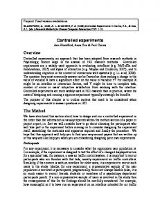
3UHOLPLQDU\UHVXOWVIRUQDUURZERWWOHQHFNH[SHULPHQW Until now, we have only elaborated one of the experiments: experiment number 10 with the narrow bottleneck. Since traffic demand exceeded the capacity of the narrow bottleneck, congestion occurred during the experiment. Thus, also part of the congested branch of the fundamental diagram can be determined from these data. The data used in this section consist of trajectories of individual pedestrians that have been determined from digital video. The trajectories of each pedestrian are described with an accuracy of 0.02 cm at each 0.1 s. Each pedestrian has a unique ID. The velocities of the pedestrians are thus easily determined from the trajectory information. Hoogendoorn and Daamen (2002) give more information on the conversion of the video data into data.

)LJXUH DF ([DPSOH WUDMHFWRULHV RI SHGHVWULDQV IRU WKUHH GLIIHUHQW PRPHQWV QDUURZ ERWWOHQHFNH[SHULPHQW 3HGHVWULDQVZDONIURPULJKW[ P WROHIW[ P 

0LFURVFRSLFSHGHVWULDQFKDUDFWHULVWLFV Figure 4 shows the trajectories of 10 pedestrians for varying traffic conditions. The time dimension has hereby omitted for the clearness of the pictures. Figure 4a shows trajectories in case the density is low and pedestrians are free to choose their paths. Figure 4b shows similar results, but in this case, densities are higher, and pedestrians were somewhat restricted in their



:LQQLH'DDPHQDQG6HUJH+RRJHQGRRUQ

53

freedom of movement. Figure 4c shows trajectories in a congested situation, in which speeds have been dropped and pedestrians have to wait to do a step forward. Figure 4 also shows that low pedestrian speed reduces the pedestrian’s ability to walk in a straight line. Furthermore, the use of the available walking space depends on the prevailing traffic conditions: when traffic conditions deteriorate, more of the available walking space is used. Figure 4 also shows interesting results inside the narrow bottleneck. It turns out that at low densities, pedestrians tend to walk in the middle of the bottleneck. When density increases, two lanes are formed, implying that the bottleneck space is used more efficiently. Because the bottleneck is narrow (width is 1.0 meter) it is impossible for pedestrians to walk next to each other. Therefore, they start walking diagonally after each other. This can be seen in the trajectories at high density, when two paths can be distinguished in the bottleneck. Let us also consider the free (or desired) speeds of the pedestrians. We assume that pedestrians walk at their free speed when not hindered by other pedestrians, i.e. when densities are very small. Having recorded all pedestrian speeds at densities lower than 0.05 P/m2, the histogram of these free speeds is shown in Figure 5. The minimum free speed we measured is 0.86 m/s, the maximum free speed is 2.18 m/s. The mean speed is 1.58 m/s. These results are comparable to earlier results of other researches. Distribution of free speeds (k