Controller Order Reduction Using the Neighborhood of Crossover Frequency Approach
ABBAS H. ZADEGAN Electrical Engineering Department Florida Atlantic University Boca Raton, FL 33431 E-mail:
[email protected]
ALI ZILOUCHIAN Electrical Engineering Department Florida Atlantic University Boca Raton, FL 33431 E-mail:
[email protected]
ABSTRACT A new model reduction approach is proposed. The order of a large-scale system is reduced within the neighborhood of its crossover frequency in order to closely preserve the gain and phase of the original system. The minimum and maximum allowable frequency about the crossover frequency of the system is determined using frequency dependent weights. Then the system is perturbed and reduced within the allowable frequency band. This approach targets model reduction at the crossover and within the allowable frequency band to maintain stability and performance. To illustrate the effectiveness of this approach, a fourth order plant model is considered and a fourth order H controller is designed, and then reduced to orders two and one for comparison. In addition, a second approach is taken so that order of the plant model is reduced to two, and then a second order controller is design through H synthesis. KEYWORDS: Model Reduction, Controller Design, Large-Scale Systems
I. INTRODUCTION In the advent of new and more complex technology, engineers often encounter large-scale systems which are numerically demanding, structurally spacious, and not very practical [1-9]. These large-scale systems in turn create a demand for smaller, less spacious, and computationally faster systems. To achieve this goal, engineers rely on model reduction technique. The problem must be approached from a realistic point of view in order to preserve the characteristics of the original system and reserve ease for troubleshooting and maintenance. Only the best fit operational frequency band must be considered. The crossover frequency, maximum and minimum allowable frequencies are considered.
Practically, a system is operational within a frequency band and outside that band the system shuts down. Simplifying the system outside the bandwidth of operation adversely effects the results. The aim of this paper is to develop an appropriate model reduction approach that preserves the gain and phase of the full order system within the bandwidth without sacrificing significant characteristics of the system such as stability and performance.
II. Plant Order Reduction Using the aforementioned concept for plant order reduction, an engineer decides a priori the frequency bandwidth 1 , 2 in which the system is operational. Next, one balances the system using a combination of modified controllability and observability Gramians and a transformation matrix [7]. Once the transformation is established, one selects the midpoint 1 2 about which the system is to be perturbed. Before proceeding with 2 singular perturbation, one can check the singular values of the Gramians and decide which states contribute the most within that frequency bandwidth. This process helps the designer to decide the order of the reduced system. Once the system is balanced and the order of the reduced system is decided, one applies the singular perturbation [8] to truncate the large-scale system to a desired reduced order within the frequency bandwidth [14]. By emphasizing the computation within a particular frequency range 1 , 2 , one can tailor a particular similarity transformation matrix T that changes the basis of the original system within that frequency range. The new basis captures all the modes dominating and governing the behavior of the system. One can show how to obtain a similarity transformation matrix T that changes the basis and, hence, the realization of the original system within the bandwidth of operation. From the new realization and singular values of the Gramians a low order system can be obtained. Consider the following n th order linear time-invariant continuous-time asymptotically stable system with the following state-space representation:
x t yt
A B
xt
C D
ut
,
(1)
where A nn , B nm , C pn , D pm are the system’s constant matrices and xt n , ut m and yt p are vectors corresponding to the states, inputs, and outputs of the system respectively. For the system in Eq. (1) with realization A, B, C, D, we can find a reduced order model with realization A r , B r , C r , D r of r th order that is both controllable and observable. The controllability and observability Gramians of the system in Eq. (1) are defined as:
0
W c e At BB e A t dt
W o e A t C Ce At dt.
(2)
0
where the (*) indicates conjugate transpose. For the system in Eq. (1) to be stable, the controllability Gramian W c and observability Gramian W o must satisfy the following Lyapunov equations [2]:
AW c W c A BB A W o W o A C C.
(3)
We apply Parseval’s theorem [10] to transform the integrals from time domain to frequency domain:
W c
1 2
Ij A 1 BB Ij A 1 d
1 2
Ij A 1 C CIj A 1 d
W o
(4)
where I is an n n identity matrix and W c and W o are controllability and observability Gramians respectively defined in frequency domain. Now, we can restrict the frequency domain to the actual bandwidth of the system, and define the controllability and observability Gramians of the system in Eq. (1) in terms of frequency over the frequency band 1 , 2 as follows: W cf
1 2
1 2
W of
2 Ij A 1 BB Ij A 1 d 1
2
Ij A 1 C CIj A 1 d
(5)
1
where symbols W cf and W of represent the controllability and observability Gramians within the specified frequency range 1 , 2 respectively. We can write the corresponding Lyapunov equation for the Gramians in Eq. (5) as follows [1-2]: AW cf W cf A BB F FBB A W of W of A C CF F C C.
(6)
where matrix F is defined by: F
2
Ij A 1 d,
(7)
1
and its complex conjugate transpose is given by: F
2
Ij A 1 d.
(8)
1
So there are two ways to compute the Gramians: (i) first method is done through Eq. (5), which cannot be easily evaluated, so we employ an iterative sum for integrals using MATLAB to find the Gramians, and (ii) the second method is done through Eqs. (6) through (8). In general, if the number of the iterative sum is sufficiently large, we can obtain a better numerical result for the Gramians. Now, if we increase the frequency bandwidth from 1 , 2 to , , we will obtain a result similar to balanced structure. Lemma: With similarity transformation matrix T and change of basis, system’s realization f, D f, C f so that the A, B, C, D can be transformed to a new balanced realization Ā f , B Gramians are equal and diagonal: of diag 1 , 2 , , n cf W (9) W
Proof: Similar to Moore’s balanced structure [7]. Using the similarity transformation T, we can define the frequency domain balanced realization of system in Eq. (1) by: f, D f, C f T 1 AT, T 1 B, CT, D Ā f , B (10) To apply singular perturbation, one reorders the system so that the eigenvalues of the system that dominate the behavior of the system will be in ascending order (the most dominant to the least dominant ) | 1 | | 2 | | n |. One partitions the balanced realization (10) into two modes, namely x t and z t to obtain the following dynamic equation:
x t
z t yt
f1 Ā f11 Ā f12 B f2 Ā f21 Ā f22 B
x t
f1 C
ut
f2 C
z t
f D
.
(11)
As 0, a homogeneous equation is obtained which allows one to eliminate z t using back substitution. The Eq. (11) can be converted solely to x as follows:
x t
yt
 B Ĉ D
x t ut
(12)
, Ĉ, D is given by: The realization Â, B Â B Ĉ D
1
Ā f11 Ā f12 Ā f22 Ā f21
f1 Ā f12 Ā 1 B f22 B f2 f1 C f2 A 1 C f22 Ā f21
(13)
f2 A 1 f C D f22 B f2
The following Fig. 1 is a brief summary of the algorithm for open-loop model reduction at any frequency level for any asymptotically stable system with realization A, B, C, D.
(A, B, C, D)
Select the desired ω1 and ω2
F=
(ω1 + ω 2 ) 2
Apply Frequency Domain Balanced Structure in [ω1 , ω2]
Apply Singular Perturbation @ F
(Ar, Br, Cr, Dr)
Fig. 1 Proposed open-loop model reduction Concepts and Properties: This proposed generalized singular perturbation method provides a good approximation at any cut off frequency level. The reduction error can be very small, contrary to any previously known model reduction techniques. The proposed technique provides a flexible tool for the designer to apply model reduction at any frequency level, in particular, at the midpoint of the bandwidth. Within the selected frequency band 1 , 2 , the reduced order model inherits a minimum amount of error since the perturbation about the mid frequency band preserves the characteristic and behavior of the original system within that neighborhood. The accuracy results from the property of the singular perturbation and the modified Gramians. In this scheme, first the system is balanced, and then singular perturbation is applied. The resulting reduced order model will capture the property of both methods, emphasizing the response of the system at the mid-frequency 1 2 level. In particular, the response of the reduced order 2 system will have the same exact value of the full order model at . This can be summed
up by the following: equation G r G.
(14)
As the frequency , the result is the same as Moore’s balanced structure, and as 0, there will be a DC match.
III. Controller Order Reduction Through frequency weights and loop shaping [11-13], one can design a stable controller Ks with robust performance that stabilizes a closed loop system Fig. 2.
Command input r(t)
Input disturbance
Output disturbance
di(t)
do(t)
Controller
Plant +
K(s) +
-
u(t)
+
Output y(t)
G(s) +
+ Sensor noise n(t)
+ +
Fig. 2 A typical closed-loop system with sensor noise and disturbances. For design of a low order controller that guarantees stability of the closed system, one employs two distinct approaches: (i) The first approach is to employ H technique [13] to design a controller for the large-scale plant model. Since these controllers usually have the same order as the plant model, for practical purposes such as troubleshooting, online implementation, and ease of computation, a low order controller is desired. Next, apply the proposed scheme at crossover frequency to reduce the order of the synthesized controller Fig. 3.
Given an nth order plant model (A, B, C, D)
Adjust weights W1 (s) and W2 (s) for the desired ω1 and ω2
Set: F =
(ω1 + ω 2 ) 2
Compute the phase PM and gain GM for desired response
Design an H4 controller (Ak, Bk, Ck, Dk) of order n. Check for robustness within frequency range [ω1, ω2]
Apply the proposed model reduction scheme @ F
No
Adjust weights
O.K.?
yes Reduced Controller (Akr, Bkr, Ckr, Dkr)
Fig. 3 Low order controller design of approach I. (ii) The second approach is to reduce the order of the large-scale plant model, and then apply H technique to design a low order controller for the reduced plant Fig. 4.
Given an nth order plant model (A, B, C, D)
Apply the proposed method to reduce the plant to rth order (Ar, Br, Cr, Dr)
Through weights W1 (s) and W2 (s) select the desired ω1 and ω2
Apply H4 controller and loop-shaping within [ω1, ω2]
Design an H4 controller (Ak, Bk, Ck, Dk) Check for robust performance within [ω1, ω2]
Apply the proposed model reduction scheme @ F
(Akr, Bkr, Ckr, Dkr)
Fig. 4 Low order controller design of approach II. The steps for H controller design is shown in Figs. 5-6, and for detailed instruction, we refer the reader to MATLAB manual. Our focus here is to combine model reduction and H technique to design a low order controller for large-scale plants.
Initial plant model (A, B, C)
Start with γ = 1, Choose weights W1(s) and W2(s)
Augment the plant matrices with the weights
Perform H∝ γ-iteration
Check for robustness in 1. H-infinity performance 2. Stability
adjust γ O.K. ?
no
yes K(s)
Fig. 5 H controller design methodology.
y2(t) y1(t)
W2(s)
di(t)
W1(s)
do(t) r(t)
e(t)
u(t)
+ K(s)
+
G(s) +
-
+ n(t) +
Fig. 6 A closed-loop system with applied loopshaping frequency weights W 1 s and W In the next section, we use Nyquist and Bode plots to illustrate the effectiveness of the proposed technique in low order controller design and model reduction of large-scale plants.
IV. Illustrative Examples Example 1. We consider the fourth order model used in papers [2,7] to demonstrate the effectiveness of model reduction at crossover frequency and within the allowable frequency bandwidth. We apply the proposed technique of open-loop model reduction to reduce the H controller model to second and first order. We compare the singular value Bode diagrams of the open loop response Ls GsK i s of the systems with the full order controller K 4 s and the reduced order controllers K i s for i 1, 2. Through Nyquist plots of Ls, we demonstrate the performance and robust stability of the reduced closed loop system within the allowable frequency range 37, 54. The results in Figs. (7-25) show the effectiveness of the proposed low order controller design scheme. Closed-Loop Model Reduction in frequency range 37, 54: Given the realization of the original plant:
Gs
A B C D
0 0 0 150
4
1 0 0 250
1
0 1 0 110
0
19
0
1
0
0 0 1 0
0
0
Low Order Controller Design in frequency range 37, 54: Approach I First we design a controller using H , which yields a controller of order four, and then reduce it to orders two and one. The results are shown in Figs. 7-13.
576s 0. 05 0. 75 ; W 2 s . 2 s 0. 5 s 120 2 The realization of the full order controller K 4 s is given by:
Choose the weights W 1 s
19 113 245 150
K 4 s
Ak Bk Ck Dk
1
1
0
0
0
0
0
1
0
0
0
0
0
1
0
0
0
0
1
4
0
The realization of the second and first order controller K 2 s.and K 1 s respectively obtained from the fourth order controller are given by:
K 2 s
K 1 s
1000 1400
15000
1400 30
1500
15000 1500
220000
1300
18000
18000 260000
,
.
Notice that the reduced controller of order one deviates a lot from the full order system, but within the frequency range [37, 54] is fine. Approach II Step 1: Reduce the plant to order two with realization: 1. 5e 001 3. 5e 00 G 2 s
3. 5e 00
6. 1e 002
2. 9e 00
6. 8e 003
6. 1e 002 6. 8e 003
2. 6e 002
With the same weights as in approach I, we obtain a stable open loop system: Step 2: Design an H stabilizing controller for the reduced plant model as follows: 8513. 0533 . K 2 s s 50s 0. 9 The results are shown in Figs. 14-25.
Conclusions The simulations, Bode plots, and Nyquist diagrams of Figs 7-25 demonstrates that at crossover frequency level and within the allowable bandwidth, the reduced order model provides almost an exact response of the original system. The Nyquist and Bode plots demonstrate that using the proposed method provides a stable controller with infinity norm performance less than one that robustly stabilizes closed-loop systems within the allowable frequency range [ 1 , 2 in the neighborhood of the crossover frequency c , where
1 c 2.
References [1] A. Zilouchian and P. Karim-Aghaee, “Frequency domain balanced structure and model
reduction of Large-scale systems,” Proceedings of American Control Conference, 1997.
[2] P. K. Aghaee, A. Zilouchian, S. Nike-Ravesh, and A. Zadegan, “Principle of frequency-domain
balanced structure in linear systems and model reduction,” Computer and Electrical Engineering, vol. 29, pp.463-477, 2003. [3] U. M. Al-Saggaf, On Model Reduction and Control of Discrete Time Systems. Ph. D. Dissertation, Stanford, CA: Department of Aeronautics and Astronautics, 1986. [4] M. Jamshidi, Large-Scale Systems: Modeling and Control. New York: Elsevier North-Holand, 1983. [5] B. D. O. Anderson and Y. Liu, “Controller reduction: concepts and approaches,” IEEE. Trans. Automat. Contr. vol. 34, pp. 802-812, 1989. [6] B. D. O. Anderson and J. B. Moore, Optimal Control: Linear Quadratic Methods. Englewood Cliffs, NJ: Prentice-Hall, 1990. [7] B. Moore,“Principle component analysis in linear systems: controllability, observability, and model reduction,” IEEE. Trans. Automat. Contr. vol. 20, pp. 17-31, 1981. [8] Y. Liu and B. D. O. Anderson,“ Singular perturbation approximation of balanced systems,” Int. J. Contr., vol. 40, pp.1379-1405, 1989. [9] G. Obinata and B.D.O. Anderson, Model Reduction for Control System Design. Springer-Verlag, Berlin, 2001. [10] R. W. Brockett, Finite Dimensional Linear Systems. New York: Wiley, 1970. [11] K. Zhou, J. C. Doyle, and K. Glover, Robust and Optimal Control. Englewood Cliffs, NJ: Prentice-Hall, 1996. [12] K. Zhou, J. C. Doyle, Essentials of Robust Control. Englewood Cliffs, NJ: Prentice-Hall, 1998. [13] W. K. Gawronski, Dynamics and Control of Structures: A Modal Approach. Springer-Verlag, Berlin, 1998. [14] J. C. Doyle, B. A. Francis, and A. R. Tannenbaum, Feedback Control Theory. New York: Macmillan, 1992.
Fig. 7 Desired open-loop Ls.
Fig. 8 The infinity norm performance.
Fig. 9 The Bode plots of Ls.
Fig. 10 The Nyquist plot of Ls.
Fig. 11 Bode plots of K i s, i 1, 2, 4.
Fig. 12 Bode plots of the closed-loop systems with K i .
Fig. 13 Nyquist plots of the closed loop systems.
Approach II results Step I: Reduce the order of the plant model
Fig. 14 Bode plot of full order plant model.
Fig. 15 Nyquist plot of the 4 th and 2 nd order plants.
Fig. 16 Step responses of the reduced and full order
Fig. 17 Impulse responses of the reduced and full order Step I: Design of a second order controller for the fourth order plant
Fig. 18 Bode plots of the weights.
Fig. 19 The desired open loop behavior.
Fig. 20 Bode plot of the open loop system.
Fig. 21 H norm performance test shows 0.51.
Fig. 22 Reduced plant of order 2.
Fig. 23 Bode plot of controller of order 2.
Fig. 24 Bode plot of open-loop Ls with K 2 s.
Fig. 25 Nyquist plot of the closed-loop system with K 2 s.