is determined by using Mihailov Criterion and numerator coefficients are obtained by using Cauer second form. We show that the mixed method is simple and ...
International Journal of Computer Applications (0975 – 8887) Volume 32– No.6, October 2011
Model Order Reduction of Interval Systems Using Mihailov Criterion and Cauer Second Form D. Kranthi Kumar
S. K. Nagar
J. P. Tiwari
Research Scholar Dept.of Electrical Engineering Institute of Technology Banaras Hindu University, Varanasi, 221005, UP, India.
Professor Dept.of Electrical Engineering Institute of Technology Banaras Hindu University, Varanasi, 221005, UP, India.
Professor Dept.of Electrical Engineering Institute of Technology Banaras Hindu University, Varanasi, 221005, UP, India.
ABSTRACT This paper presents a new mixed method for reducing the large scale interval systems using the Mihailov Criterion and Cauer second form. The reduced order model of denominator is determined by using Mihailov Criterion and numerator coefficients are obtained by using Cauer second form. We show that the mixed method is simple and guarantees the stability of the reduced model if the original system is stable. A numerical examples are illustrated and verified its stability.
Keywords Mihailov Criterion, Cauer second form, Reduced order, Stability, Mixed method.
1. INTRODUCTION Model order reduction of interval systems has been considered by several researchers. The technique of Routh approximation [1] based on direct truncation guarantees the stability of reduced order model. γ-δ Routh approximation [2] evaluated for order reduction. Hwang [3] has proposed comments on the computation aspects of interval Routh approximation. Sastry et al [4] has proposed γ table approximation to decreasing complexity of the γ-δ Routh algorithm. Yuri Dolgin suggested another generalization of direct routh table truncation method [5] for interval systems. He proved that the existing generalization of direct truncation of Routh fails to produce a stable system. But S-F.Yang commented [6] on Yuri Dolgin‟s method that it cannot guarantee the stability of lower order interval systems. To overcome all these problems Yuri Dolgin added some conditions [7] for getting the stability of reduced order through Routh approximation. To improve the effectiveness of model order reduction many mixed methods are proposed recently [8-11]. In the present paper, model order reduction of interval systems is carried out by using mixed method. The denominator of the reduced model is obtained by Mihailov Criterion and the numerator is obtained by Cauer second form. Thus the stability of the reduced order model is guaranteed, if the higher order interval system is asymptotically stable. The brief outline of this paper is as follows: Section 2 contains problem statement. Section 3 contains proposed method. Error analysis done in section 4. Numerical examples are presented in section 5 and t conclusion in section 6.
2. PROBLEM STATEMENT Let the transfer function of a higher order interval systems be [𝑝 0− , 𝑝 0+ ] + 𝑝 1− , 𝑝 1+ 𝑠+ …… + 𝑝 𝑛−−1 ,𝑝 𝑛+−1 𝑠 𝑛 −1
𝐺𝑛 𝑠 =
𝑞 0− ,𝑞 0+ + 𝑞 1− ,𝑞 1+ 𝑠+ …….+ 𝑞 𝑛− ,𝑞 𝑛+ 𝑠 𝑛
=
𝑁 (𝑠) 𝐷 (𝑠)
(1) where [𝑝𝑖− , 𝑝𝑖+ ] for i = 0 to n-1 and [𝑞𝑖− , 𝑞𝑖+ ] for i = 0 to n are known as scalar constants. The reduced order model of a transfer function be considered as + − + − + 𝑟−1 𝑢− 0 ,𝑢 0 + 𝑢 1 ,𝑢 1 𝑠+ ……+[𝑢 𝑟−1 ,𝑢 𝑟−1 ]𝑠
𝑅𝑟 𝑠 =
𝑣0− ,𝑣0+ + 𝑣1− ,𝑣1+ 𝑠+ ……+ 𝑣𝑟− ,𝑣𝑟+ 𝑠 𝑟
=
𝑁𝑟 𝑠 𝐷𝑟 𝑠
(2)
where [𝑢𝑗− , 𝑢𝑗+ ] for j= 0 to r-1and [𝑣𝑗− , 𝑣𝑗+ ] for j = 0 to r are known as scalar constants. The rules of the interval arithmetic have been defined in [12], as follows. Let [e , f] and [g , h] be two intervals. Addition: [e , f] + [g , h] = [e + g , f + h] Subtraction: [e , f] – [g , h] = [e – h , f – g] Multiplication: [e , f] [g , h] = [Min (eg, eh, fg, fh), Max (eg, eh, fg, fh)] Division: 𝑒 ,𝑓 𝑔 ,
= 𝑒 ,𝑓
1
,
1 𝑔
3. PROPOSED METHOD The proposed method consists of the following steps for obtaining reduced order model. Step 1: Determination of the denominator polynomial of the 𝑘 𝑡 order reduced model: Substituting s = jω in D(s) and separating the denominator into real and imaginary parts, − + − + 𝐷 (𝑗𝑤) = [𝑐11 , 𝑐11 ] + 𝑐12 , 𝑐12 𝑗𝜔 − + + … . + 𝑐1,𝑛+1 , 𝑐1,𝑛+1 (𝑗𝜔)𝑛
17
International Journal of Computer Applications (0975 – 8887) Volume 32– No.6, October 2011
− + − + − + = 𝑐11 , 𝑐11 − 𝑐13 , 𝑐13 ] 𝜔 2 + … … . + 𝑗𝜔 ( 𝑐12 , 𝑐12 𝜔− − + 2 𝑐14 , 𝑐14 𝜔 + … … )
= ξ (𝜔) + j𝜔 η(𝜔) (3)
Step 2: Determination of the numerator coefficients of the 𝑘 𝑡 order reduced model by using Cauer second form: Coefficient values from Cauer second form [𝑝− , 𝑝+ ] (p =1 , 2 , 3 . . . . k) are evaluated by forming Routh array as
where ω is the angular frequency, rad/sec. ξ (ω) = 0 and ɳ (ω) = 0, the frequencies which are − + intersecting 𝜔0 = 0, ± 𝜔1− , 𝜔1+ , … … . ±[ 𝜔𝑛−1 , 𝜔𝑛−1 ] are − + − + obtained, where [𝜔1 , 𝜔1 ] ≺ [𝜔2 , 𝜔2 ] ≺ … . . ≺ − [𝜔𝑛−1 , 𝜔𝑛+−1 ] . Similarly substituting s = j𝜔 in 𝐷𝑘 𝑠 , then obtains
1− , 1+ =
− + 𝑐11 , 𝑐11 − + 𝑐21 , 𝑐21
− + 𝑐11 , 𝑐11 − + 𝑐21 , 𝑐21
− + 𝑐12 , 𝑐12 ……. − + 𝑐22 , 𝑐22 ……
2− , 2+ =
− + 𝑐21 , 𝑐21 − + 𝑐31 , 𝑐31
− + 𝑐21 , 𝑐21 − + 𝑐31 , 𝑐31
− + 𝑐22 , 𝑐22 ……. − + 𝑐32 , 𝑐32 ……
3− , 3+ =
− + 𝑐31 , 𝑐31 − + 𝑐41 , 𝑐41
− + 𝑐31 , 𝑐31 − + 𝑐41 , 𝑐41
− + 𝑐32 , 𝑐32 ……. − + 𝑐42 , 𝑐42 ……
𝐷𝑘 𝑗𝜔 = 𝝓 𝜔 + 𝑗𝜔 𝝍 (𝜔) (4) where − + − + 𝜙 𝜔 = [𝑑11 , 𝑑11 ] − 𝑑13 , 𝑑13 𝜔2 + …. and
...... ................. (9)
− + − + 𝜓 𝜔 = [𝑑12 , 𝑑12 ] − 𝑑14 , 𝑑14 𝜔2 + ….
Put 𝜙 (𝜔) = 0 and 𝜓 (𝜔) = 0, then we get k number of roots and it must be positive and real and alternately distributed along the w axis. The first k numbers of frequencies are 0, − + 𝜔1− , 𝜔1+ , 𝜔2− , 𝜔2+ , . … .. , [𝜔𝑘−1 , 𝜔𝑘−1 ] are kept unchanged and the roots of 𝜙 (𝜔) = 0 and 𝜓 (𝜔) = 0.
𝜓 𝜔 = + 𝜆− 𝜔 2 − 𝜔22 , 𝜔22 2 , 𝜆2 2 2 𝜔6 , 𝜔6 … (6)
.............
......................... ..............
The first two rows are copied from the original system numerator and denominator coefficients and rest of the elements are calculated by using well known Routh algorithm. [𝑐𝑖𝑗− , 𝑐𝑖𝑗+ ] = − + − + − + 𝑐(𝑖−2,𝑗 +1) , 𝑐(𝑖−2,𝑗 +1) − 𝑖−2 , 𝑖−2 [𝑐(𝑖−1,𝑗 +1) , 𝑐(𝑖−2,𝑗 +1) ]
(10)
Therefore, 𝜙 𝜔 = 𝜆1− , 𝜆1+ 𝜔 2 − 𝜔12 , 𝜔12 𝜔52 , 𝜔52 … (5)
............
where i = 3,4,. . . . . and j = 1,2, . . . . 𝜔 2 − 𝜔32 , 𝜔32
𝜔2 −
𝑖− , 𝑖+ =
− + [𝑐𝑖,1 ,𝑐𝑖,1 ] − + [𝑐(𝑖+1,1) ,𝑐(𝑖+1,1) ]
; i = 1,2,3,………k
(11) − + The coefficient values of 𝑑𝑖,𝑗 , 𝑑𝑖,𝑗 (j = 1,2,.....(k+1))] 2
𝜔 −
𝜔42 , 𝜔42
2
𝜔 −
+ For finding the coefficient values of [𝜆1− , 𝜆1+] and [𝜆− 2 , 𝜆2 ] are − calculated from ξ (0) = 𝜙 (0) and ɳ 𝜔1 , 𝜔1+ = − + − − + 𝜓 𝜔1 , 𝜔1 . keeping these values of [𝜆1 , 𝜆+ 1 ] and [𝜆2 , 𝜆2 ] in equations (5) and (6), respectively, 𝜙 (𝜔) and 𝜓 (𝜔) are obtained and 𝐷𝑘 (𝑗𝜔) is obtained as
𝐷𝑘 𝑗𝜔 = 𝝓 𝜔 + 𝑗𝜔 𝝍 (𝜔) (7) Now replace j𝜔 by s, then the 𝑘 𝑡 order reduced denominator 𝐷𝑘 (𝑠) is obtained as − + − + 𝐷𝑘 (𝑗𝜔) = [𝑑11 , 𝑑11 ] + 𝑑12 , 𝑑12 𝑠 + − + 𝑘 … . + 𝑑1,𝑘+1 , 𝑑1,𝑘+1 (𝑠) (8)
Of the equation (8) and Cauer quotients [𝑝− , 𝑝+ ] (p = 1. 2, . . . k) of the the equation (9) are matched for finding the coefficients of numerator of the reduced model 𝑅𝑘 (𝑠). The inverse routh array is constructed as − + [𝑑(𝑖+1,1) , 𝑑(𝑖+1,1) ]=
+ [𝑑 𝑖−,1 ,𝑑 𝑖,1 ]
[ 𝑖− , + 𝑖 ]
(12) i = 1,2, . . .,k and k ≤ n − + [𝑑(𝑖+1,𝑗 +1) , 𝑑(𝑖+1,𝑗+1) ] =
− + ( 𝑑 −𝑖,𝑗 +1 ,𝑑 +𝑖,𝑗 +1 −[𝑑 (𝑖+2,𝑗 ) ,𝑑 (𝑖+2,𝑗 ) ]
[ 𝑖− , 𝑖+ ]
(13) where i = 1. 2, . . . . , (k-j) and j = 1,2 ,. . . . , (k-1) Using the above equations, the numerator coefficients of the reduced model are obtained and numerator is written as
18
International Journal of Computer Applications (0975 – 8887) Volume 32– No.6, October 2011 − + − + − + 𝑁𝑘 𝑠 = 𝑑21 , 𝑑21 + 𝑑22 , 𝑑22 𝑠 + ⋯ + [𝑑2𝑘 , 𝑑2𝑘 ]𝑠 𝑘−1 (14)
𝑁2 𝑠 = 11.1949, 20.3706 𝑠 + [14.1674, 16.9413] Step 7: The reduced order model 𝑅2 (𝑠) is given as
𝑅2 𝑠 =
4. Error Analysis The integral square error (ISE) in between the transient responses of higher order system (HOS) and Lower order system (LOS) and is given by: ISE =
∞ [𝑦(𝑡) 0
11.1949,20.3706 𝑠+[14.1674 ,16.9413 ] 17..0011 ,18.0007 𝑠 2 + 31.3826 ,33.6111 𝑠+[20.3061 ,21.7052 ]
− 𝑦𝑟 (𝑡)]² dt
(15) where, y (t) and 𝑦𝑟 (t) are the unit step responses of original system 𝐺𝑛 𝑠 and reduced order system 𝑅𝑘 𝑠 .
5. Numerical Examples Example 1: Consider a third order system described by the transfer function [13] 𝐺3 𝑠 =
2,3 𝑠 2 + 17.5,18.5 𝑠+[15,16]
(16)
2,3 𝑠 3 + 17,18 𝑠 2 + 35,36 𝑠+[20.5,21.5]
Step 1: Put s = j𝜔 in the denominator D (s) D (j𝜔) = ([20.5, 21.5] – [17, 18]𝜔 2 ) + j𝜔 ([35, 36] – [2, 3]𝜔 2 ) Step 2: The intersecting frequencies are [𝜔𝑖−, 𝜔𝑖+ ] = 0, 1.0929, 1.0981 , [3.4641, 4.1833]
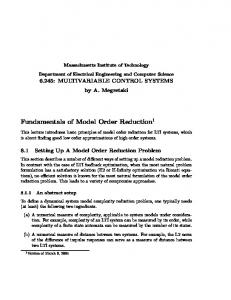
Fig. 1 : Step Response of original model and ROM
Step 3: Following the procedure given in section 3, the denominator of the second order model is taken as + 2 𝐷2 𝑗𝜔 = 𝜆− 1 , 𝜆1 𝜔 − 1.0929, 1.9081
𝜆1−, 𝜆1+
Here = − 17.0011, 18.0007 [31.3826, 33.6111]
2
+ + 𝑗𝜔 [𝜆− 2 , 𝜆2 ],
and
+ 𝜆− 2 , 𝜆2
=
+ Step 4: Substitute the values of [𝜆1−, 𝜆1+] and [𝜆− 2 , 𝜆2 ] in step 3 and also substitute j𝜔 = s.
Table 1. Comparison of Reduced Order Models Method of reduction
Order
ISE for lower limit errL
ISE for upper limit errU
Proposed Algorithm
0.0089
0.0113
G.V.S.S Sastry [3]
0.2256
0.0095
Hence, the denominator D(s) is given by 𝐷2 𝑠 = 17. .0011, 18.0007 𝑠 2 + 31.3826, 33.6111 𝑠 + [20.3061, 21.7052] Step 5: Using the Cauer second form as described in the section 3, it is obtained [1− , 1+] = [1.2812, 1.4333] [2− , 2+] = [1.1046, 1.8859] − + [𝑑21 , 𝑑21 ] = [14.1674, 16.9413] − + [𝑑22 , 𝑑22 ] = [11.1949, 20.3706] are obtained.
Step 6: Numerator of second order system is written as
The step response of second order model is obtained by the proposed method and compared with second order model. Example 2: Consider a third order system described by the transfer function [16] 𝐺3 𝑠 =
1,1 𝑠 2 + 3.3,6.5 𝑠+[2.7,10] 1,1
𝑠3 +
8.5,8.6 𝑠 2 + 18,18.2 𝑠+[10.25,10.76]
(17) Step 1: Put s = j𝜔 in the denominator D (s) D(j𝜔)= ([10.25, 10.76]–[8.5, 8.6]𝜔 2 ) + j𝜔([18, 18.2]–[1, 1]𝜔 2)
19
International Journal of Computer Applications (0975 – 8887) Volume 32– No.6, October 2011 Step 2: The intersecting frequencies are
Table 2. Comparison of Reduced Order Models
[𝜔𝑖−, 𝜔𝑖+ ] = 0, 1.0981, 1.1185 , [4.2426, 4.2661] Step 3: Following the procedure given in section 3, the denominator of the second order model is taken as + 2 𝐷2 𝑗𝜔 = 𝜆− 1 , 𝜆1 𝜔 − 1.0929, 1.9081
Here [𝜆1−, 𝜆1+]
2
+ + 𝑗𝜔 [𝜆− 2 , 𝜆2 ],
= − 8.1934, 8.9235 and
+ 𝜆− 2 , 𝜆2 = [16.749, 16.9942] + Step 4: Substitute the values of [𝜆1−, 𝜆1+ ] and [𝜆− 2 , 𝜆2 ] in step 3 and also substitute j𝜔 = s.
Hence, the denominator D(s) is given by 𝐷2 𝑠 = 8.1934, 8.9235 𝑠 2 + 16.749, 16.9942 𝑠 + 9.8796, 11.1633 Step 5: Using the Cauer second form as described in the section 3, it is obtained [1− , 1+] = [1.025, 3.9852] [2− , 2+] = [−1.2652, 0.6749] − + [𝑑21 , 𝑑21 ] = [2.4791, 10.8910] − + [𝑑22 , 𝑑22 ] = [0.1535, 24.9778] are obtained.
Step 6: Numerator of order system is written as 𝑁2 𝑠 = 0.1535, 24.9778 𝑠 + [2.4791, 10.8910] Step 7: The reduced second order model 𝑅2 (𝑠) is given as 𝑅2 𝑠 =
0.1535 ,24.9778 𝑠+ 2.4791,10.8910 8.1934,8.9235 𝑠 2 + 16.749,16.9942 𝑠+ 9.8796 ,11.1633
The step response of second order model is obtained by the proposed method and compared with second order model
Method of Order reduction
ISE for lower limit errL
ISE for upper limit errU
Proposed Algorithm
0.0264
1.0314
G.Saraswathi [8]
0.0034
0.0364
6. CONCLUSION In this paper Mihailov criterion and Cauer second form is employed for order reduction. The reduced model of denominator polynomial is obtained by using Mihailov criterion and the numerator is determined by cauer second form. The proposed method guarantees the stability of reduced model if the original system is stable. This proposed method is conceptually simple and comparable with other well known methods. Two examples are taken from the literature and compared with other methods by using ISE.
7. REFERENCES [1] B. Bandyopadhyay, O. Ismail, and R. Gorez, “Routh Pade approximation for interval systems,” IEEE Trans. Automat. Contr., pp. 2454–2456, Dec1994. [2] B. Bandyopadhyay.: „γ-δ Routh approximations for interval systems‟, IEEE Trans. Autom. Control, pp. 1127-1130, 1997. [3] C. Hwang and S.-F. Yang, “Comments on the computation of interval Routh approximants,” IEEE Trans. Autom. Control, vol. 44, no. 9, pp.1782–1787, Sep. 1999. [4] G V K Sastry, G R Raja Rao and P M Rao. „Large Scale Interval System Modelling Using Routh Approximants.‟ Electronics Letters, vol 36, no 8, pp. 768. April 2000. [5] Y. Dolgin and E. Zeheb, “On Routh-Pade model reduction of interval systems,” IEEE Trans. Autom. Control, vol. 48, no. 9, pp. 1610–1612, Sep. 2003. [6] S. F. Yang, “Comments on „On Routh-Pade model reduction of interval systems‟,” IEEE Trans. on Automatic Control, vol. 50, no. 2, pp.273-274, 2005. [7] Y. Dolgin, “Author‟s Reply,” IEEE Trans. Autom. Control, vol. 50, no. 2, pp. 274-275, Feb. 2005. [8] G.Saraswathi, “ A Mixed Method for Order Reduction of Interval Systems,” International Conference on Intelligent and Advanced Systems, pp. 1042-1046, 2007. [9] Yan Zhe Penngfei Bi Zhiqiang Zhang and Liwei Niu, “ Improved algorithm of model order reduction of large scale internal system, The 6th International Forum on strategic technology, pp:716- 719, Aug 22-24, 2011.
Fig.2.Step Response of original model and ROM
[10] D.Kranthi kumar, S. K. Nagar and J. P. Tiwari, “Model Order Reduction of Interval Systems Using Mihailov Criterion and Routh Approximations”, International journal of engineering science and technology , Vol. 3 No. 7, pp. 5593-5598, July 2011.
20
International Journal of Computer Applications (0975 – 8887) Volume 32– No.6, October 2011 [11] D. Kranthi kumar, S. K. Nagar and J. P. Tiwari, “Model Order Reduction of Interval Systems Using Mihailov Criterion and Factor Division Method”, International journal of computer applications ,Volume 28– No.11, pp. 4-8, August 2011 [12] E.Hansen, “Interval arithmetic in matrix computations, Part I,” SIAM J. Numerical Anal., pp. 308-320, 1965.
8. BIOGRAPHIES D. Kranthi Kumar was born in Guntur, A.P, India in 1986. He received the degree of B.E from SIR. C. R. Reddy College of Engineering in 2008 and received the degree of M.Tech in Electrical Engineering from IT-BHU, Varanasi, in 2010 and presently pursuing Ph.D in Electrical Engineering at IT-BHU, Varanasi, India. He is life member in System Society of India (SSI) and student member in Institute of Engineers (Ireland).
of Technology, Banaras Hindu University (IT-BHU), Varanasi, India In 1976 and 1978; and PhD in Electrical Engineering from University of Roorkee (IIT Roorkee), India in 1991. He is currently Professor in Electrical Engineering at IT-BHU, Varanasi, India. His main research includes digital control, model order reduction and discrete event systems. He has published many papers in national & International conferences & Journals. J. P. Tiwari was born in Deoria, U.P, India in 1947. He received the degrees of B.E. and M.E. from University of Roorkee, India in 1968 and 1971. Ph.D in Electrical Engineering from Banaras Hindu University, India in 1991. He is currently Professor, Head of the Department in Department of Electrical Engineering at IT-BHU, Varanasi, India. His main research includes Control systems, Robotics, Instrumentation, Control Systems, Adaptive control. He has published many papers in National & International conferences and journals.
S. K. Nagar was born in Varanasi, India in 1955. He received the degrees of B.Tech and M.Tech from the Institute
21