Controlling Complex Networks with Compensatory Perturbations

Controlling Complex Networks with Compensatory Perturbations Sean P. Cornelius1 , William L. Kath2,3 , and Adilson E. Motter1,3 1 Department

of Physics and Astronomy,Northwestern University, Evanston, IL 60208, USA of Engineering Sciences and Applied Mathematics, Northwestern University, Evanston, IL 60208, USA 3 Northwestern Institute on Complex Systems, Northwestern University, Evanston, IL 60208, USA

arXiv:1105.3726v1 [q-bio.MN] 18 May 2011

2 Department

The response of complex networks to perturbations is of utmost importance in areas as diverse as ecosystem management, emergency response, and cell reprogramming. A fundamental property of networks is that the perturbation of one node can affect other nodes, in a process that may cause the entire or substantial part of the system to change behavior and possibly collapse. Recent research in metabolic and food-web networks has demonstrated the concept that network damage caused by external perturbations can often be mitigated or reversed by the application of compensatory perturbations. Compensatory perturbations are constrained to be physically admissible and amenable to implementation on the network. However, the systematic identification of compensatory perturbations that conform to these constraints remains an open problem. Here, we present a method to construct compensatory perturbations that can control the fate of general networks under such constraints. Our approach accounts for the full nonlinear behavior of real complex networks and can bring the system to a desirable target state even when this state is not directly accessible. Applications to genetic networks show that compensatory perturbations are effective even when limited to a small fraction of all nodes in the network and that they are far more effective when limited to the highest-degree nodes. The approach is conceptually simple and computationally efficient, making it suitable for the rescue, control, and reprogramming of large complex networks in various domains.

Introduction Complex systems such as power grids, cellular networks, and food webs are often modeled as networks of dynamical units. In such complex networks, a certain incidence of perturbations and the consequent impairment of the function of individual units—whether genes, power stations, or species—are largely unavoidable in realistic situations. While local perturbations may rarely disrupt a complex system, they can propagate through the network as the system accommodates to a new equilibrium. This in turn often leads to system-wide re-configurations that can manifest themselves as genetic diseases [1, 2], power outages [3, 4], extinction cascades [5, 6], traffic congestions [7, 8], and other forms of large-scale failures [9, 10]. A fundamental characteristic of large complex networks, both natural and man-made, is that they operate in a decentralized way. On the other hand, such networks have either evolved or been engineered to inhabit stable states in which they perform their functions efficiently. The existence of stable states indicates that arbitrary initial conditions converge to a relatively small number of persistent states. Such states are generally not unique and can change in the presence of large perturbations. Because complex networks are decentralized, upon perturbation the system can spontaneously go to a state that is less efficient than others available. For example, a damaged power grid undergoing a large blackout may still have other stable states in which no blackout would occur, but the perturbed system does not converge to those states. We suggest that many large-scale failures are determined by the convergence of the network to a “bad” state rather than by the unavailability of “good” states. Here we explore the hypothesis that one can design physically admissible compensatory perturbations to direct a network to a desirable state even when it would spontaneously go to an undesirable (“bad”) state. An important precedent comes from the study of food-web networks, where perturbations caused by invasive species or climate change can lead to the subsequent extinction of numerous species. Recent research predicts that a significant fraction of these extinctions can be prevented by the targeted suppression of specific species in the system [11]. Another precedent comes from the study of metabolic networks of single-cell organisms, where perturbations caused by genetic or epigenetic defects can lead to nonviable strains, which are unable to reproduce. The knockdown or knockout of specific genes has been predicted to mitigate the consequence of such defects and often recover the ability of the strains to grow [12]. These findings have analogues in power grids, where perturbations caused by equipment malfunction or operational errors can lead to large blackouts, but the appropriate shedding of power can substantially reduce subsequent failures [13, 14]. Therefore, the concept underlying our hypothesis is supported by recent research on physical [14, 15], biological [12, 16], and ecological networks [11]. In these studies, the identification of compensatory perturbations relied either on simple models of the real system [14, 15] or on using heuristic arguments [11, 12]. The question we pose is whether compensatory perturbations can be systematically identified for a general network of dynamical units. Our solution to this problem is based on the observation that associated with each desirable state there is a region of initial conditions that converge to it—the so-called “basin of attraction” of that state. Given a network that is at (or will approach) an undesirable state, the conceptual problem is thus reduced to the identification of a perturbation in the state of the system that can bring it to the attraction basin of the desired stable state (the target state). Once there, the system will evolve spontaneously to the target. However, this 2

perturbation must be physically admissible and is therefore subject to constraints—in the examples above, certain genes can be down-regulated but not over-expressed, the populations of certain species can only be reduced, and changes in power flow are limited by capacity and generation capability. Under such constraints, the identification of a point within the basin of attraction of the target state is a highly nontrivial task. This is so because complex networks are high-dimensional dynamical systems and it is generally impossible to identify the boundaries of a basin of attraction in more than just a handful of dimensions. The approach introduced here overcomes this difficulty and is able to identify compensatory perturbations in the absence of any a priori information about the location of the attraction basin of the target state. This is done systematically, without resorting to trial-and-error. The approach is effective even when only exploiting resources available in the network, which usually forbids bringing the system directly to the desired stable state. This often limits the search to perturbations that are locally deleterious, such as the temporary inactivation of a node. Interestingly, applications of our method show that such locally deleterious perturbations can be tailored to lead to globally advantageous effects. The approach is general and can be used to both control a network in the imminence of a failure and to reprogram a network even in the absence of any impending failure.

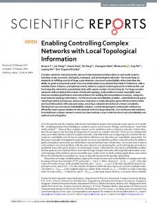
Results Figure 1A-C illustrates the problem that we intend to address. The dynamics of a network is best studied in the state space, where we can follow the time evolution of individual trajectories and characterize the stable states of the whole system. Figure 1A represents a network that would spontaneously go to an undesirable state, and that we would like to bring to a desired stable state by perturbing at most three of its nodes (highlighted). Using x = (x1 , ..., xn ) to represent the dimensions of the state space, Fig. 1B shows how this perturbation applied at a certain time t0 , changing the state of the system from x0 to x00 , would lead to an orbit that asymptotically goes to the target state. As an additional constraint, assume that the activity of the nodes can only be reduced (not increased) by this perturbation. Then, in the subspace corresponding to the nodes that can be perturbed, the set of points X that can be reached by eligible compensatory perturbations forms a cubic region, as shown in Fig. 1C. The target state itself is outside this region, meaning that it cannot be directly reached by any eligible perturbation. However, the basin of attraction of the target state may have points inside the region of eligible perturbations (Fig. 1B), in which case the target state can be reached through perturbations that bring the system to one of these points; once there, the system will spontaneously evolve towards the target state. This scenario is representative of the conditions under which it is important to identify compensatory perturbations, and leads to a very clear conclusion: a compensatory perturbation exists if and only if the region formed by eligible compensatory perturbations overlaps with the basin of attraction of the target. However, there is no general method to identify basins of attraction (or this possible overlap) in high-dimensional state spaces typical of complex networks. Indeed, despite significant advances, numerical simulations are computationally prohibitive and analytical methods, such as those based on Lyapunov stability theorems, offer only rather conservative estimates and are not yet sufficiently developed to be used in this context [17, 18]. Accordingly, our approach does not assume any information about the location of the 3

attraction basins and addresses a problem that, as further explained below, cannot be solved by existing methods from control theory.

Control procedure for networks The dynamics of a complex network can often be represented by a set of coupled ordinary differential equations. We thus consider an N -node network whose n-dimensional dynamical state x is governed by dx = F(x). (1) dt The example scenario we envision is the one in which this network has been perturbed at a time prior to t0 , driving it to a state x0 = x(t0 ) in the attraction basin Ω(xu ) of an undesirable state xu . The compensatory perturbation that we seek to identify consists of a judiciously-chosen perturbation x0 → x00 to be implemented at time t0 , where x00 belongs to the basin of attraction Ω(x∗ ) of a desirable state x∗ . For simplicity, we assume that xu and x∗ are fixed points, although the approach we develop extends to other types of attractors. In the absence of any constraints it is always possible to perturb x0 such that x00 ≡ x∗ . However, as illustrated above, usually only constrained compensatory perturbations are allowed in real networks. These constraints encode practical considerations and often take the form of mandating no modification to certain nodes, while limiting the direction and extent of the changes in others. The latter is a consequence of the relative ease of removing versus adding resources to the system. We thus assume that the constraints on the eligible perturbations can be represented by the vectorial expressions g(x0 , x00 ) ≤ 0 and h(x0 , x00 ) = 0,

(2)

where both the equality and the inequality are assumed to apply to each component. In a food web, for example, admissible compensatory perturbations may only reduce the populations of certain unendangered species, while leaving those of the endangered ones unchanged. For concreteness, we focus on constraints of the form x00j ≤ x0j for accessible nodes, and x00j = x0j for the other nodes, although the approach we develop accommodates general, nonlinear constraints. We propose to construct compensatory perturbations iteratively from small perturbations, as shown in Fig. 1D-E. Given a dynamical system in the form (1) and an initial state x0 at time t0 , a small perturbation δx0 evolves to δx(t) = M(x0 , t) · δx0 at time t. The matrix M(x0 , t) is the solution of the variational equation dM/dt = DF(x) · M subject to the initial condition M(x0 , 0) = 1, and is generally invertible [19]. Given the time tc of closest approach of the perturbed orbit to the target x∗ , we can in principle use the inverse transformation, δx0 = M−1 (x0 , tc ) · δx(tc ), (3) to determine the perturbation δx0 to the initial condition x0 that, among the admissible perturbations satisfying |δx0 | ≤ 1 , will render x(tc ) + δx(tc ) closest closest to x∗ (Fig. 1D). This is a good approximation for small 1 , and hence for small changes in the initial conditions; the error can in fact be calculated from the matrix of second derivatives and verified numerically by direct integration. Large perturbations can then be built up by iterating the process: every time δx0 is calculated, the current initial state, x00 , is updated to x00 + δx0 , and a new δx0 is calculated starting from the new initial condition (Fig. 1E). 4

The problem of identifying a perturbation δx0 that incrementally moves the orbit toward the target under the given constraints is then cast as a constrained optimization problem (see Methods). Once found, the optimal incremental perturbation is applied to the current initial condition, x00 → x00 +δx0 , giving the initial state for the next iteration. At this point, we test whether the new state lies in the target’s basin of attraction by integrating the system (1) over a long time τ . If the resulting orbit reaches a small ball of radius κ around the target, we declare success and terminate the procedure. Otherwise, we identify the closest approach point in a time window t0 ≤ t ≤ t0 + T , where T is a time limit determined beforehand, and repeat the procedure. Now, it may be the case that no compensatory perturbation can be found, e.g., if the feasible region X does not intersect the target basin Ω(x∗ ). To account for this, we automatically terminate our search if the system is not controlled within a fixed number of iterations (see Methods). Before considering the application to networks, we first illustrate our method using an example in two dimensions, where the basins of attraction (and hence the possible compensatory perturbations) can be easily calculated and visualized. Figure 2 shows the state space of the system, which has two stable states: xA on the left and xB on the right. The system is defined by the potential U (x1 ) = exp(−γx21 )(bx21 + cx31 + dx41 ) and frictional dissipation η, where γ = 1, b = −1, c = −0.1, d = 0.5, η = 0.1, and x2 = x˙ 1 . The method is illustrated for two different initial states under the constraint that admissible perturbations have to satisfy x00 ≤ x0 , i.e., one cannot increase either variable. For the initial state in the basin of state xA (Fig. 2A), no admissible perturbation exists that can bring the system directly to the target xB , on the right, since that would require increasing x1 . However, our iterative procedure builds an admissible perturbation vector that shifts the state of the system to a branch of the basin Ω(xB ) lying on the left of that point. Then, from that instant on the autonomous evolution of the system will govern the trajectory’s approach to the target xB , on the right. This example illustrates how compensatory perturbations that move in a direction away from the target—the only ones available under the given constraints—can be effective in controlling the system, and how they are identified by our method. The other example shown illustrates a case in which the perturbation to an initial state on the right crosses an intermediate basin, of xB , before it can reach the basin of the target, xA (Fig. 2B). The linear approximation fails at the crossing point, but convergence is nonetheless assured by the constraints imposed on δx0 (see Methods).

Control of genetic networks We now turn to compensatory perturbations in complex networks. We focus on networks of diffusively coupled units, a case that has received much attention in the study of spontaneous synchronization [20]. We take as a base system the genetic regulatory subnetwork shown in Fig. 3A (inset), consisting of two genes wired in a circuit. The state of the system is determined by the expression levels of the genes, represented by the variables x1 , x2 ≥ 0. The associated dynamics obeys dx1 xm Sm = a1 m 1 m + b1 m − k 1 x1 + f 1 , (4) dt x1 + S x2 + S m dx2 xm Sm = a2 m 2 m + b2 m − k 2 x2 + f 2 , (5) dt x2 + S x1 + S m where the first two terms for each gene capture the self-excitatory and mutually inhibitory interactions represented in Fig. 3A, respectively, while the final two terms represent linear 5

decay and a basal activation rate of the associated gene’s expression. Models of this form have been used extensively to describe the transition between progenitor stem cells and differentiated cells [21–23]. For a wide range of parameters, this system exhibits three stable states: a state (xB ) characterized by comparable expression of both genes (the stem cell state), and two states (xA and xC ) characterized by the dominant expression of one of the genes (differentiated cell states). Figure 3 and subsequent results correspond to the symmetric choice of parameters a1,2 = 0.5, b1,2 = 1, k1,2 = 1, f1,2 = 0.2, S = 0.5, and m = 4. We assume that compensatory perturbations are limited to gene down-regulations, i.e., x00 ≤ x0 . Admissible compensatory perturbations do not exist (and hence cannot be identified) from some other initial states close to the axis in the basin of xA,C having xC,A as target, indicating that the expression of that gene is too low to be rescued by compensatory perturbations. But xB can be reached even in these cases, and thus so can xA,C if we let the system evolve after a perturbation into Ω(xB ) and then perturb it again into Ω(xC,A ), meaning that we need the conversion from the differentiated state to the stem cell state before going to the other differentiated state. We construct large genetic networks by coupling multiple copies of the two-gene system described above. Such networks may represent cells in a tissue or culture coupled by means of factors exchanged through their microenvironment or medium. Specifically, we assume that each copy of this genetic system can be treated as a node of the larger network. The dynamics of a network consisting of N such systems is then governed by dxi ε X = f (xi ) + Aij [xj − xi ], dt di j

(6)

where x˙ i = f (xi ) is the vectorial form of the dynamics of node i as described by Eqs. (4)(5), the parameter ε > 0 is the overall coupling strength, and di is the degree (number of connections) of node i. The structure of the network itself is encoded in the adjacency matrix A = (Aij ). We focus on randomly generated networks with both uniform and preferential attachment rules (Methods), which serve as models for homogeneous and heterogeneous degree distributions, respectively. We use ~x = (xi ) to denote the state of the network, with ~xA , ~xB , and ~xC denoting the states in which all nodes are at state xA , xB , and xC , respectively. The states ~xA , ~xB , and ~xC are fixed points of the full network dynamics in the 2N -dimensional state space and, by arguments of structural stability, we can conclude they are also stable and have qualitatively similar basins of attraction along the coordinate planes xi if the coupling strength ε is weak. While we focus on these three states, it follows from the same arguments that in this regime there are 3N − 3 other stable states in the network. Under such conditions, compensatory perturbations between ~xA , ~xB , and ~xC are guaranteed to exist, and hence this class of networks can also serve as a benchmark to test the effectiveness and efficiency of our method in finding compensatory perturbations in systems with a large number of nodes. A general compensatory perturbation in this network is illustrated in Fig. 3B, where different intensities indicate different node states. Applied to the initial state ~xA and target ~xB for ε = 0.05, the method is found to be effective in 100% of the cases for the 10, 000 networks tested, with N ranging from 10 to 100. Moreover, the computation time and number of iterations for these tests confirm that our method is also computationally efficient for large networks. Computation time grows approximately quadratically with N (Fig. 3C), as expected since each iteration requires the integration of O(N 2 ) equations. √ The number of iterations grows as the square root of N (Fig. 3D), in agreement with the N 6

scaling of |~xA − ~xB | and of the distances between other invariant sets. This leads to the asymptotic scaling N 5/2 for the computation time, which is not onerous since the control of one network requires the identification of only one compensatory perturbation. This should be compared to the O(exp(N )) time that would be required to determine the basin of attraction at fixed resolution by exhaustive sampling of the state space. These properties are representative of more general conditions. The efficiency and effectiveness of our approach are expected to be relevant not only for large genetic networks, but also for large real networks in general, such as food webs and power grids, where the characteristic time to failure after the initial perturbation is large relative to the expected time scales to identify compensatory perturbations. In the preceding analysis, we allowed all nodes in the network to be perturbed, thus providing an upper bound for the computational time. In a realistic situation we may assume that only a subset of the network is made available to perturbations. While compensatory perturbations are not expected to exist under such constraints for very small ε, they become abundant for larger coupling strengths. Figure 4 shows the success rate in directing the system from ~x0 = ~xB to ~x∗ = ~xA for several network sizes and a varying number of nodes k in the control set, i.e., the set of nodes available to be perturbed. For ε = 1, as considered in these case, the success rate increases monotonically with k, as expected, but it is frequently possible to identify an eligible compensatory perturbation using a small number of nodes in the network. For example, for networks of 50 nodes, approximately 40% of all randomly selected 10-node control sets will lead to successful control, for both homogeneous (Fig. 4A) and heterogeneous (Fig. 4B) networks. Naturally, for the network to be controlled it suffices to find a single successful control set, indicating that the networks will often be rescued by a much smaller fraction of nodes. From a comparison between Fig. 4A and Fig. 4B it follows that, for control sets formed by randomly selected nodes, heterogeneous networks are more likely to be controlled than homogeneous ones if the size of the control set is small, while the opposite is true if the control set is large. The analysis below will allow us to interpret this property of heterogeneous networks as a consequence of the possibility of having a very high-degree node in small control sets and a tendency to have a large number of low-degree nodes in large control sets. But what distinguishes a successful control set from a set that fails to control the network? Figure 5 shows that the probability of success is strongly determined by node degree. This is clear from the probability that a node appears in a successful control set as a function of its degree d (Fig. 5A), which increases approximately linearly for both homogeneous and heterogeneous networks. This is even more evident in the dependence of the success rate on the average degree hdi of the control set (Fig. 5B). The success rate exhibits a relatively sharp transition from zero to one as hdi increases, which starts near the peak of the distribution of average degrees for random control sets (Fig. 5B, background histograms). As shown in Fig. 5C for a homogeneous network, the success rate of control sets involving a given node correlates strongly with degree even across relatively small degree differences. This confirms both that compensatory perturbations can be identified for a large fraction of control sets and that successful control sets show an enrichment of high-degree nodes. Because successful control sets tend to have a significantly higher fraction of high-degree nodes, increased success rate can be achieved by biasing the selection of control-set nodes towards high degrees. This is demonstrated in Fig. 6, where the rate of success increases dramatically when the control set is formed by the highest-degree nodes in the network. For example, for the control sets formed by 20% of the nodes, the success rate approaches

7

100% for all network sizes considered, more than doubling when compared to randomly selected control sets. This increase is more pronounced for more heterogeneous networks, as illustrated for control sets limited to 10% of the nodes (Fig. 6), which is expected from Fig. 5 and the availability of higher degree nodes in such networks. This enhanced controllability of degree-heterogeneous networks for targeted node selection is important in view of the prevalence of heterogeneous degree distributions in natural and engineered networks. We emphasize that these conclusions follow from our systematic identification of compensatory perturbations, and that they cannot be derived from the existing literature. Note that our approach is fundamentally different from those usually considered in control theory, both in terms of methods and applicability. Optimal control [24], for example, is based on identifying an admissible (time-dependent) control u(t) such that the modified system dx/dt = F + u will optimize a given cost function. Control of chaos [25], which is used to convert an otherwise chaotic trajectory into a periodic one, is based on the continuous application of unconstrained small time-dependent perturbations to align the stable manifold of an unstable periodic orbit with the trajectory of the system. Approach to the relevant orbit can be facilitated by the method of targeting [26], which, like control of chaos itself, can only be applied to move within the same ergodic component. Here, in contrast, we bring the system to a different component, to a state that is already stable, and we do so using one (or few) finite-size perturbations, which are forecast-based rather than feedback-based. Our approach is suited to a wide range of processes in complex networks, which are often amenable to modeling but offer limited access to interventions, making the use of punctual interventions that benefit from the natural stability of the system far more desirable than other conceivable alternatives.

Discussion The dynamics of large natural and man-made networks are usually highly nonlinear, making them complex not only with respect to their structure but also with respect to their dynamics. This is particularly manifest when the networks are brought away from equilibrium, as in the event of a strong perturbation. Nonlinearity has been the main obstacle to the control of such systems. Progress has been made in the development of algorithms for decentralized communication and coordination [27], in the manipulation of two-state Boolean networks [28], in network queue control problems [29], and other complementary areas. Yet, the control of far-from-equilibrium networks with self-sustained dynamics, such as metabolic networks, power grids, and food webs, has remained largely unaddressed. Methods have been developed for the control of networks hypothetically governed by linear dynamics [30]. But although linear dynamics may approximate an orbit locally, it does not permit the existence of different stable states observed in real networks and does not account for basins of attraction and other global properties of the state space. These global properties are crucial because they underlie network failures and, as shown here, also provide a mechanism for the control of numerous networks. The possibility of directing a complex network to a predefined dynamical state offers an unprecedented opportunity to harness such highly structured systems. We have shown that this can be achieved under rather general conditions by systematically designing compensatory perturbations that, without requiring the computationally-prohibiting explicit identification of the basin boundaries, take advantage of the full basin of attraction of the 8

desired state, thus capitalizing on (rather than being obstructed by) the nonlinear nature of the dynamics. While our approach makes use of constrained optimization [31], the question at hand cannot be formulated as a simple optimization problem in terms of an aggregated objective function, such as the number of active nodes. Maximizing this number by ordinary means can lead to local minima or transient solutions that then fall back to asymptotic states with larger number of inactive nodes. A priori identification of the stable state that enjoys the desired properties is thus an important step in our formulation of the problem. Applications of our framework show that the approach is effective even when compensatory perturbations are limited to a small subset of all nodes in the network, and when constraints forbid bringing the network directly to the target state. This is of outmost importance for applications because, in large networks, perturbed states in which the desired state is outside the range of admissible perturbations is expected to be the rule rather than the exception. From a network perspective, this leads to counterintuitive situations in which the compensatory perturbations oppose the direction of the target state and consist, for example, of suppressing nodes whose activities are already diminished relative to the target, but that lead the system to eventually evolve towards that target. These results are surprising in light of the usual interpretation that nodes represent “resources” of the network, to which we intentionally (albeit temporarily) inflict damage with a compensatory perturbation. From the state space perspective, the reason for the existence of such locally deleterious perturbations that have globally beneficial effects is that the target’s basin of attraction, being nonlocal, can extend to the region of feasible perturbations even when the target itself does not. Our results based on randomly-generated networks also show that control is far more effective when focused on high-degree nodes. The effect is more pronounced in more heterogenous networks, making it particularly relevant for applications to real systems, which are known to often exhibit fat-tailed degree distributions [32, 33]. More generally, we posit that the rate of successful control on a network will be strongly biased towards nodes with high centrality, including degree centrality, as shown here, and possibly other measures of centrality in the case of networks that deviate from random, such as closeness and betweenness. This suggests that in the situation where only a limited intervention is possible, one should focus primarily on central nodes in order to direct the entire network to a desired new state. We have demonstrated, moreover, that even when all nodes in the network are perturbed, the identification of compensatory perturbations is computationally inexpensive and scales well with the size of the network, allowing the analysis of very large networks. We have motivated our problem assuming that the network is away from its desirable equilibrium due to an external perturbation. In that context, our approach provides a methodology for real-time rescue of the network, bringing it to a desirable state before it reaches a state that can be temporarily or permanently irreversible, such as in the case of cascades of overload failures in power grids or cascades of extinctions in food webs, respectively. We suggest that this can be important for the conservation of ecological systems and for the creation of self-healing infrastructure systems. More generally, as illustrated in our genetic network examples, our approach also applies to change the state of the network from one stable state to another stable state, thus providing a mechanism for “network reprogramming”. As a context to interpret the significance of this application, consider the reprogramming of differentiated (somatic) cells from a given tissue to pluripotent stem cell state, which can then differentiate into cells of a different type of tissue. The seminal experiments

9

demonstrating this possibility involved continuous overexpression of specific genes [34], which is conceivable even under the hypothesis that cell differentiation is governed by the loss of stability of the stem cell state [22]. However, the recent demonstration that the same can be achieved by temporary expression of few proteins [35] indicates that the stem cell state may have remained stable (or metastable) after differentiation, allowing interpretation of this process in the context of the interventions considered here. This is relevant because a very small fraction of a population of treated cells is found to undergo the transition back to the stem cell state, suggesting that much could be learned from a modeling approach capable of identifying the perturbations most likely to direct the cellular network to adopt a new stable state. While induced pluripotency is an example par excellence of network reprograming, the same concept extends far beyond this particular system. Taken together, our results provide foundation for the control and rescue of network dynamics, and as such are expected to have implications for the development of smart traffic and power-grid networks, of ecosystems and Internet management strategies, and of new interventions to control the fate of living cells.

Methods Constraints on incremental perturbations. The iterative procedure behaves well as long as the linearization involved in Eq. (3) remains valid at each step. The incremental perturbation at the point of closest approach, δx(tc ), selected under constraints (2) alone will generally have a nonzero component along a stable subspace of the orbit x(t), which will result in δx0 larger than δx(tc ) by a factor O(exp |λtsc (tc − t0 )|), where λtsc is the finite-time Lyapunov exponent of the eigendirection corresponding to the smallest-magnitude eigenvalue of M(x0 , tc ). In a naive implementation of this algorithm, to keep δx0 small for the linear transformation to be valid, the size of δx(tc ) would be negligible, leading to negligible progress. This problem is avoided by optimizing the choice of δx(tc ) under the constraint that the size of δx0 is bounded above. Another potential problem is when the perturbation causes the orbit to cross an intermediate basin boundary before reaching the final basin of attraction. All such events can be detected by monitoring the difference between the linear approximation and the full numerical integration of the orbit, without requiring any prior information about the basin boundaries. Boundary crossing is actually not a problem because the closest approach point is reset to the new side of the basin boundary. To assure that the method will continue to make progress, we solve the optimization problem under the constraint that the size of δx0 is also bounded below, which means that we accept increments δx0 that may temporarily increase the distance from the target (to avoid back-and-forth oscillations, we also require the inner product between two consecutive increments δx0 to be positive). These upper and lower bounds can be expressed as 0 ≤ |δx0 | ≤ 1 .

(7)

This can lead to |δx(tc )|  1 due to components along the unstable subspace, but in such cases the vectors can be rescaled after the optimization. At each iteration, the problem of identifying a perturbation δx0 that incrementally moves the orbit toward the target under constraints (2) and (7) is then solved as a constrained optimization problem.

10

Nonlinear optimization. The optimization step of the iterative control procedure consists of finding the small perturbation δx0 that minimizes the remaining distance between the target, x∗ , and the system orbit x(t) at its time of closest approach, tc . Constraints are used to both define the admissible perturbations (2) and also, as described in the previous paragraph, limit the magnitude of δx0 (7). The optimization problem to identify δx0 can then be succinctly written as: min

|x∗ − (x(tc ) + M(x00 , tc ) · δx0 )|

s.t.

(8)

g(x0 , x00 + δx0 ) ≤ 0

(9)

h(x0 , x00 + δx0 ) = 0

(10)

0 ≤ |δx0 | ≤ 1

(11)

δx0 · δxp0 ≥ 0,

(12)

where (12) is enforced starting from the second iteration, and δxp0 denotes the incremental perturbation from the previous iteration. Formally, this is a nonlinear programming (NLP) problem, the solution of which is complicated by the nonconvexity of the constraint (11) (and possibly (9) and (10)). Nonetheless, a number of algorithms have been developed for the efficient solution of NLP problems, among them Sequential Quadratic Programming (SQP) [36]. This approach solves (8) as the limit of a sequence of quadratic programming subproblems, in which the constraints are linearized in each sub-step. For all calculations, we used the SQP algorithm [37] implemented in the SciPy scientific programming package (http://www.scipy.org/). Note that this implementation does not require inverting matrix M (cf. Eq. (3)). Comparison with backward integration. Our approach should be compared with an apparently simpler alternative. Rather than keeping track of the variational matrix M(x0 , t), which requires the integration of n2 additional differential equations at every iteration, one could imagine using backwards integration of a trajectory starting at x(tc ) + δx(tc ) to identify a suitable initial perturbation. This alternative procedure suffers the critical drawback that, for a particular choice of δx(tc ) (magnitude and direction), it is not certain that the time-reversed orbit will ever strike the feasible region defined by (2). This is particularly so in realistic situations where only a fraction of the nodes are accessible to perturbations, resulting in a feasible region of measure zero in the full n-dimensional state space. Termination criteria and parameters. In all simulations, the control procedure is terminated if the updated initial condition attracts to within κ = 0.01 of the target state within τ = 10, 000 time units. Otherwise, we terminate the search if a compensatory perturbation is not found after a fixed number of iterations, which we set to be I = 1, 000. In general this number should be of the order of L/0 , where L is the characteristic linear size of the feasible region. For each iteration, we use T = 10 time units within the integration step that identifies tc , which was estimated based on the time to approach the undesirable stable state. In the examples of Fig. 2, we used the parameters 0 = 0.001 and 1 = 0.01 for the optimization step. To lighten the computational burden in our Monte Carlo analysis, we used a more relaxed choice of 0 = 0.005 and 1 = 0.05 for the genetic 11

networks presented in Figs. 3–6. Construction of genetic networks. The networks are grown starting with a d-node connected seed network, by iteratively attaching a new node P and connecting this node to each pre-existing node i with probability d × Pi , where i Pi = 1. The connections are assumed to be unweighted and undirected. We reject any iteration resulting in a degree-zero node, thereby ensuring that the final N -node network is connected and has average degree ≥ 2d for large N . Networks are generated for both uniform attachment probability, where Pi = 1/N s and N s is the number of nodes P in the network at iteration s, and for linear preferential attachment, where Pi = kis / j kjs and kis is the degree of node i at iteration s. The former leads to networks with asymptotically exponential distribution of degrees, which we refer to as homogeneous networks, while the latter leads to networks with asymptotically power-law distribution of degrees, which we refer to as heterogeneous networks [32]. By construction, the resulting average degree is essentially the same for both homogeneous and heterogeneous networks. In our simulations, we focused on networks with d = 2. Acknowledgments The authors thank Jie Sun for illuminating discussions and the Brockmann Group for use of their computer cluster. This work was supported by the National Science Foundation under Grant DMS-1057128 and the National Cancer Institute under Grant 1U54CA143869-01.

12

[1] Motter AE, Improved network performance via antagonism: From synthetic rescues to multidrug combinations. BioEssays 32, 236–245 (2010). [2] Barab´asi A-L, Gulbahce N, Loscalzo J, Network medicine: A network-based approach to human disease. Nature Rev Genet 12, 56–68 (2011). [3] Carreras BA, Newman DE, Dobson I, Poole AB, Evidence for self-organized criticality in a time series of electric power system blackouts. IEEE T Circuits-I 51, 1733–1740 (2004). [4] Buldyrev SV, Parshani R, Paul G, Stanley HE, Havlin S, Catastrophic cascade of failures in interdependent networks. Nature 464, 1025–1028 (2010). [5] Pace ML, Cole JJ, Carpenter SR, Kitchell JF, Trophic cascades revealed in diverse ecosystems. Trends Ecol Evol 14, 483–488 (1999). [6] Scheffer M, Carpenter S, Foley JA, Folke C, Walker B, Catastrophic shifts in ecosystems. Nature 413, 591–596 (2001). [7] Helbing D, Traffic and related self-driven many-particle systems. Rev Mod Phys 73, 1067–1141 (2001). [8] Vespignani A, Predicting the behavior of techno-social systems. Science 325, 425–428 (2009). [9] May RM, Levin SA, Sugihara G, Complex systems: Ecology for bankers. Nature 451, 893–895 (2008). [10] Haldane AG, May RM, Systemic risk in banking ecosystems. Nature 469, 351–355 (2011). [11] Sahasrabudhe S, Motter AE, Rescuing ecosystems from extinction cascades through compensatory perturbations. Nat Commun 2, 170 doi:10.1038/ncomms1163 (2011). [12] Motter AE, Gulbahce N, Almaas E, Barab´asi A-L, Predicting synthetic rescues in metabolic networks. Mol Syst Biol 4, 168 (2008). [13] Anghel M, Werley KA, Motter AE, Stochastic model for power grid dynamics. Proceedings of the 40th International Conference on System Sciences, HICSS’07 Vol. 1, 113 (2007). [14] Carreras BA, Lynch VE, Dobson I, Newman DE, Critical points and transitions in an electric power transmission model for cascading failure blackouts. Chaos 12, 985–984 (2002). [15] Motter AE, Cascade control and defense in complex networks. Phys Rev Lett 93, 098701 (2004). [16] Cornelius SP, Lee JS, Motter AE, Dispensability of Escherichia coli’s latent pathways. Proc Natl Acad Sci USA 108, 3124–3129 (2011). [17] Genesio R, Tartaglia M, Vicino A, On the estimation of asymptotic stability regions: State of the art and new proposals. IEEE T Automat Contr 30, 747–755 (1985). [18] Kaslik E, Balint AM, Balint St, Methods for determination and approximation of the domain of attraction. Nonlinear Analysis 60, 703–717 (2005). [19] Ott E, Chaos in Dynamical Systems (Cambridge Univ Press, Cambridge, UK, 2002). [20] Pecora LM, Carroll TL, Master stability functions for synchronized coupled systems. Phys Rev Lett 80, 2109–2112 (1998). [21] Roeder I, Glauche I, Towards an understanding of lineage specification in hematopoietic stem cells: A mathematical model for the interaction of transcription factors GATA-1 and PU.1. J Theor Biol 241, 852–865 (2006). [22] Huang S, Guo YP, May G, Enver T, Bifurcation dynamics in lineage-commitment in bipotent progenitor cells. Dev Biol 305, 695–713 (2007). [23] Wang J, Xu L, Wang E, Huang S, The potential landscape of genetic circuits imposes the arrow of time in stem cell differentiation. Biophys J 99, 29–39 (2010). [24] Kirk DE, Optimal Control Theory (Dover Publications Inc, Mineola, NY, 2004).

13

[25] Ott E, Spano M, Controlling chaos. Phys Today 48, 34–40 (1995). [26] Bollt EM, Targeting control of chaotic systems, in Chaos and Bifurcations Control: Theory and Applications. eds. Chen G, Yu X, Hill DJ, (Springer-Verlag, Berlin, 2003). [27] Bullo F, Cort´es J, Mart´ınez S, Distributed Control of Robotic Networks: A Mathematical Approach to Motion Coordination Algorithms, Applied Mathematics Series (Princeton Univ Press, Princeton, NJ, 2009). [28] Shmulevich I, Dougherty ER, Probabilistic Boolean Networks: The Modeling and Control of Gene Regulatory Networks (SIAM, Philadelphia, PA, 2009). [29] Meyn SP, Control Techniques for Complex Networks (Cambridge Univ Press, Cambridge, UK, 2008). [30] Lin C-L, Structural controllability. IEEE T Automat Contr 201–208 (1974). [31] Bazaraa MS, Sherali HD, Shetty CM, Nonlinear Programming: Theory and Algorithms (John Wiley & Sons Inc, Hoboken, NJ, 2006). [32] Barab´asi A-L, Albert R, Emergence of scaling in random networks. Science 286, 509–512 (1999). [33] Caldarelli G, Scale-Free Networks: Complex Webs in Nature and Technology (Oxford University Press, Oxford, UK, 2007) [34] Takahashi K, Yamanaka S, Induction of pluripotent stem cells from mouse embryonic and adult fibroblast cultures by defined factors. Cell 126, 663–676 (2006). [35] Kim D, et al. Generation of human induced pluripotent stem cells by direct delivery of reprogramming proteins. Cell Stem Cell 4, 472–476 (2009). [36] Boggs PT, Tolle JW, Sequential quadratic programming. Acta Numerica 4, 1–51 (1995). [37] Kraft D, A software package for sequential quadratic programming. Technical report DFVLRFB, Institut f¨ ur Dynamik der Flugsysteme, Oberpfaffenhofen, 88–28 (1998).

14

A

C

B target,

D

E

target

controlled orbit

target

feasible region

feasible region

FIG. 1: Schematic illustration of the network control problem. (A) Network portrait. The goal is to drive the network to a desired state by perturbing a control set consisting of one or more nodes. (B) State space portrait. In the absence of control, the network at an initial state x0 evolves to an undesirable equilibrium in the n-dimensional state space (red curve). By perturbing this state (orange arrow), the network reaches a new state x00 that evolves to the desired target state (blue curve). (C) Constraints. In general, there will be constraints on the types of compensatory perturbations that one can make. In this example, one can only perturb three out of n dimensions (equality constraints), which we assume to correspond to a thee-node control set, and the dynamical variable along each of these three dimensions can only be reduced (inequality constraints). This results in a set of eligible perturbations, which in this case forms a cube within the three-dimensional subspace of the control set. The network is controllable if and only if the corresponding slice of the target’s basin of attraction (blue volume) intersects this region of eligible perturbations (grey volume). (D, E) Iterative construction of compensatory perturbations. (D) A perturbation to the current initial condition (magenta arrow) corresponds to a perturbation of the resulting orbit (green arrow) at the point of closest approach to the target. At every step, we seek to identify a perturbation that brings this point, and hence the orbit, closer to the target. (E) This process generates orbits that approach increasingly closer to the target (dashed curves), and is repeated until a perturbed state x00 is identified that evolves to the target. The resulting compensatory perturbation x00 − x0 (orange arrow) brings the system to the attraction basin of the target without any a priori information about its location, and allows directing the network to a state that is not directly accessible by any eligible perturbation.

15

B

A

FIG. 2: Illustration of the control process in two dimensions. Yellow and blue represent the basins of attraction of the stable states xA and xB , respectively, while white corresponds to unbounded orbits. (A and B) Iterative construction of the perturbation for an initial state in the basin of xA with xB as a target (A), and for an initial state on the right side of both basins with xA as a target (B). Dashed and continuous lines indicate the original and controlled orbits, respectively. Red arrows indicate the full compensatory perturbations. Individual iterations of the process are shown in the insets (for clarity, not all iterations are included).

16

A 1

C

2 Activation Inhibition

D B s eou tan on n o sp oluti ev

com pe pert nsatory urba tion

spontaneous evolution

FIG. 3: Control of genetic networks. (A) State space of the two-gene subnetwork represented in the inset, where the red curves mark the boundaries between the basins of xA , xB , and xC , and the arrows indicate the local vector field. (B) Illustration of compensatory perturbation on complex genetic networks, where each node is a copy of the two-gene system. We are given an initial network state ~x0 representing the expression levels of the N gene pairs (color coded), and this state evolves to a stable state of the network ~xu (top path). The goal is to knockdown one or more genes to reach a new state ~x00 that instead evolves to a target stable state ~x∗ 6= ~xu (bottom path). (C and D) Average computation time (C) and average number of iterations (D) required to control networks of N nodes with initial state ~x0 = ~xA and target ~x∗ = ~xB , demonstrating the good scalability of the algorithm. Each point represents an average over 1, 000 independent realizations of homogeneous networks.

17

A

B

FIG. 4: Control of networks using a small fraction of all nodes. The dynamics follows (6) for ε = 1 and the control is illustrated for bringing the network from state ~xB to state ~xA . (A) Probability that an N -node homogeneous network can be controlled by perturbing only k randomly selected nodes. (B) Corresponding results for heterogeneous networks with the same average degree (see Methods). Each point represents an average over 1, 000 network realizations for one control set each. Thus, for control sets consisting of randomly selected nodes, heterogeneous networks are more likely to be controlled than homogeneous networks if the size of the control set is small. This should be contrasted with the case of control sets formed by the highest-degree nodes (see Fig. 6), where heterogeneous networks are more likely to be controlled for both small and large control sets.

18

A

B

C 10 0.32 0.28 0.24 0.20

8 6 4

0.16 0.12

2

FIG. 5: Enrichment of high-degree nodes in successful control sets. (A) Probability that a given node of degree d is present in a successful control set for homogeneous (top) and heterogeneous (bottom) networks. This probability is scaled as P (d) = s(d)/N (d), where s is the number of times (counting multiplicity) a node of degree d appears in a successful control set, while N (d) is the total number of such nodes appearing in all successfully-controlled networks. (B) Dependence of the success rate on the average degree of the control set. Probability (red) for homogeneous (top) and heterogeneous (bottom) networks that a random set of 20% of the nodes can be used to control the corresponding network as a function of the average degree hdi in the set. The background of each panel (light blue) shows the distribution of hdi for randomly formed control sets. (C) Relation between success rate (left) and node degree (right) in an example network. The color bars show the percentage of successful control sets involving the given node (red) and the degree of the node (blue). Each point in panels A and B correspond to an average over 5, 000 network realizations sampled 10 times while the statistics in panel C are based on sampling the given network 10, 000 times, where N = 50 and k = 10 in all cases. The dynamics, coupling strength, and initial and target states are the same considered in Fig. 4. It follows that the ability to control a network correlates strongly with the degrees of the nodes in question.

19

A

B

FIG. 6: Increase in rate of successful control through high-degree nodes. (A and B) Probability of successfully controlling homogeneous (A) and heterogeneous (B) networks with a control set formed by a fraction of randomly selected nodes (gray) or by the same fraction of highest-degree nodes (orange). The fraction of nodes accessible in the control set is selected to be only 10% (circles) and 20% (diamonds) of the network. Each point represents an average over 2, 000 independent network realizations for initial state ~xB and target state ~xA , for the dynamics and coupling strength considered in Fig. 4. Biasing the intervention towards high-degree nodes dramatically improves the ability to control the network, permitting success with a small number of nodes where control through randomly selected nodes or low-degree nodes would fail.

20