Spectrum of Controlling and Observing Complex Networks

Spectrum of Controlling and Observing Complex Networks Gang Yan1† , Georgios Tsekenis1† , Baruch Barzel2 , Jean-Jacques Slotine3 , Yang-Yu Liu4,5 , Albert-

arXiv:1503.01160v1 [physics.soc-ph] 3 Mar 2015

L´aszl´o Barab´asi1,4,5,6∗

1

Center for Complex Network Research and Department of Physics, Northeastern University,

Boston, Massachusetts 02115, USA 2

Department of Mathematics, Bar-Ilan University, Ramat-Gan 52900, Israel

3

Department of Mechanical Engineering and Department of Brain and Cognitive Sciences, Mas-

sachusetts Institute of Technology, Cambridge, Massachusetts 02139, USA 4

Department of Medicine and Division of Network Medicine, Brigham and Women’s Hospital,

Harvard Medical School, Boston, Massachusetts 02115, USA 5

Center for Cancer Systems Biology, Dana Farber Cancer Institute,Boston, Massachusetts 02115,

USA 6

Center for Network Science, Central European University, H-1051 Budapest, Hungary

†

These authors contributed equally to this work.

∗

Corresponding author. Email: [email protected]

1

Observing and controlling complex networks are of paramount interest for understanding complex physical, biological and technological systems. Recent studies have made important advances in identifying sensor or driver nodes, through which we can observe or control a complex system. Yet, the observation uncertainty induced by measurement noise and the energy cost required for control continue to be significant challenges in practical applications. Here we show that the control energy cost and the observation uncertainty vary widely in different directions of the state space. In particular, we find that if all nodes are directly driven, control is energetically feasible, as the maximum energy cost increases sublinearly with the system size. If, however, we aim to control a system by driving only a single node, control in some directions is energetically prohibitive, increasing exponentially with the system size. For the cases in between, the maximum energy decays exponentially if we increase the number of driver nodes. We validate our findings in both model systems and real networks. Our results provide fundamental laws that deepen our understanding of diverse complex systems.

Introduction Many natural and man-made systems can be represented as networks1–3 , where nodes are the system’s components and links describe the interactions between them. Thanks to these interactions, perturbations of one node can alter the states of the other nodes. This property has been exploited to control a network, i.e., to move it from an initial state to a desired final state4–6 by manipulating the state variables of only a subset of its nodes7 . Such control processes7–19 play an important role in the regulation of protein expression20 , the coordination of moving robots21 , and the inhibition 2

of undesirable social contagions22 . At the same time the interdependence between nodes means that the states of a small number of sensor nodes contain sufficient information about the rest of the network, so that we can reconstruct the system’s full internal state by accessing only a few outputs23 . This can be utilized for biomarker design in cellular networks, or to monitor in real time the functionality of infrastructural24 and social-ecological25 systems for early warning of failures or disasters26 .

While recent advances in driver and sensor node identification constitute unavoidable steps towards controlling and observing real networks, in practice we continue to face significant challenges: the control of a large network may require a vast amount of energy12–14 and measurement noise27 causes uncertainties in the observation process. To quantify these issues we formalize the dynamics of a controlled network with N nodes and ND external control inputs as4–7 ˙ x(t) = Ax(t) + Bu(t),

(1)

where the vector x(t) = [x1 (t), x2 (t), . . . , xN (t)]T describes the states of the N nodes at time t. In (1) xi (t) can represent the concentration of a metabolite in a metabolic network28 , the geometric state of a chromosome in a chromosomal interaction network10 , or the belief of an individual in opinion dynamics22, 29 . The vector u(t) = [u1 (t), u2 (t), . . . , uND (t)]T represents the external control inputs, and B is the input matrix with Bij = 1 if the control input uj (t) is imposed on node i. The adjacency matrix A captures the interactions between the nodes, including the possibility of self-loops Aii representing the self-regulation of node i.

The system (1) can be driven from an initial state xo to any desired final state xd within 3

the time t ∈ [0, τ ] using an infinite number of possible control inputs u(t). The optimal input vector aims to minimize the energy cost4

Rτ 0

ku(t)k2 dt, which captures the energy of electronic

and mechanic systems or the amount of effort required to control biological and social systems. If at t = 0 the system is in state xo = 0, the minimum energy required to move the system to point xd in the state space is4, 12, 13 E(τ ) = xTd G−1 c (τ )xd , where Gc (τ ) =

Rτ 0

(2)

T

eAt BB T eA t dt is the symmetric controllability Gramian. When the system

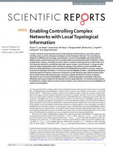
is controllable all eigenvalues of Gc (τ ) are positive. Eq. (2) indicates that for a network A and an input matrix B the control energy E(τ ) also depends on the desired state xd . Consequently, driving a network to various directions in the state space requires different amounts of energy. For example, to move the weighted network of Fig. 1a to the three different final states xd with kxd k = 1, we inject the optimal signals u(t) shown in Fig. 1b onto node 1, steering the system along the trajectories shown in Fig. 1c. The corresponding minimum energies are shown in Fig. 1d. The control energy surface for all normalized desired states is an ellipsoid, implying that the required energy varies dramatically as we move the system in different directions.

Results As real systems normally function near a stable state, i.e., all eigenvalues of A are negative30 , the control energy E(τ ) decays quickly to a nonzero stationary value when the control time τ increases12 . Henceforth we focus on the control energy E ≡ E(τ → ∞) and the controllability Gramian G ≡ Gc (τ → ∞).

4

Given a network A and an input matrix B, the controllability Gramian G is unique, embodying all properties related to the control of the system. To uncover the direction of the state space requiring different energies, we explore the eigen-space of G. Denote by Ei the eigen-energies, i.e., the minimum energy required to drive the network to G’s eigen-directions. According to Eq. (2) Ei = 1/µi with µi corresponding to G’s eigenvalues. Generally, the energy surface for a network with N nodes is a super-ellipsoid spanned by G’s N eigen-directions. To determine the distribution of these eigen-energies we decompose the adjacency matrix as A = V ΛV T , where V represents the eigenvectors of A and Λ = diag{−λ1 , −λ2 , . . . , −λN } are the eigenvalues. (For stable undirected networks all eigenvalues of A are negative, thus we denote the eigenvalues by −λi so that the absolute eigenvalues are λi > 0 for all i.) We sort the absolute eigenvalues in ascending order 0 < λ1 < λ2 < . . . < λN , and find that (SI Sec. I) G = V [(V T BB T V ) ◦ C]V T ,

(3)

where ◦ denotes Hadamard product, i.e., (X ◦ Y )ij = Xij Yij , and C is a matrix with entries Cij =

1 . λi +λj

For a given network, (3) captures the impact of the input matrix B on the control

properties of the system, allowing us to analyze the distribution of eigen-energies for different number of driver nodes and determine the required energy for each direction.

Controlling all nodes If we can control all nodes, i.e., ND = N , B becomes a unit diagonal matrix. In this case G = V diag{ 2λ1 i }V T and the eigen-directions of the controlled system are the same as the network’s eigenvectors. Thus Ei = 2λi and p(E) = p(λ), i.e., the distribution of eigen-energies is identical to the distribution of the network’s absolute eigenvalues. We add self-loops as Aii = −(δ+ 5

PN

j=1

Aij )

where δ > 0 is a small perturbation to ensure that all eigenvalues of A are negative. This scheme has been widely used in previous studies on dynamical processes taking place on networks, such as opinion dynamics22 , synchronization31 , and control12 . For networks with degree distribution1–3 p(k) ∼ k −γ the distribution of A’s absolute eigenvalues also obeys a power law32, 33 p(λ) ∼ λ−γ (see SI Sec. II A). Consequently, p(E) ∼ E −γ ,

(4)

indicating that most directions of the state space are easily controlled, requiring a small E. A few 1

directions require considerable energy. The most difficult direction needs34 Emax ∼ N γ−1 . The fact that Emax is sub-linear in N for γ > 2 indicates that the required energy remains bounded, hence there are no significant energetic barriers for control with ND = N . As shown in Fig. 2b, for the scale-free model35 and the S. cerevisiae protein-protein interaction36 networks p(E) indeed follows a power law; in contrast for the Erd¨os-R´enyi random network37 and the US power grid38 p(E) are bounded (Fig. 2a), as predicted by γ → ∞ in (4), requiring even less energy for control.

Controlling a single node If each node has a nonidentical self-loop we can control an undirected network by driving only a single node39 . In this case V T BB T V = {Vih Vjh } ∼ O(1/N ), where h is the index of the single driver node. Thus V T BB T V can be viewed as a small perturbation to the matrix C in (3). The statistical behavior of G’s eigenvalues is mainly determined by the eigenvalues of C, whose distribution can be approximated as p(E) ∼ 1/(1 + 1/E)E −1 (see SI Sec. IIIA, B for details). Therefore, p(E) ∼ E −1 6

(5)

for large E. Eq. (5) predicts that, to drive a network of N nodes with a single driver node, the most difficult direction in the state space requires Emax ∼ eN energy (SI Sec. III C). This exponential N -dependence makes the control of large networks (N ) in the most difficult direction energetically infeasible. For validation we also consider the complementary cumulative distribution p> (E) =

R Emax E

p(E 0 )dE 0 . Based on (5) we obtain p> (E) ∼ (ln Emax − ln E), decreasing linearly

with ln E. This is confirmed for both Erd¨os-R´enyi and scale-free network models in Fig 2(c). For the numerical feasibility we also test the distribution on two moderate-size empirical networks: a terrorist communication network40 where Aij represents the interaction frequency between i and j; and a mutualistic ecological network41 where weighted edges describe interaction strength between species. As shown in Fig 2(d), although there are deviations due to degree correlations42 , the presence of communities43 and nestedness44 characterizing these networks, the corresponding eigen-energies span over a hundred of orders of magnitude and are reasonably well approximated by (5).

Controlling a finite fraction of nodes ˆ ∼ e(1−γ)Eˆ where Eˆ ≡ ln E. Thus, if ND = N , p(E) ˆ is When p(E) ∼ E −γ , the distribution p(E) ˆ is an exponential (one-peak) distribution as γ > 2 in (4); if ND = 1, as p(E) ∼ E −1 in (5), p(E) a uniform distribution. To understand the transition from (4) for ND = N to (5) for ND = 1, we ˆ when 1 < ND < N , i.e., controlling a finite fraction of nodes. investigate the distribution p(E) ˆ has multiple peaks (Fig. 3a), which is induced by the gaps in the In this case, we find that p(E) eigen-energy spectrum (Fig. 3b). For ND /N = 0.6, there is a gap separating the eigen-energies into two bands and the lower band contains ND eigen-energies. This gap leads to two peaks in the 7

ˆ as shown in Fig. 3c. When we have fewer driver nodes (ND /N decreases), the distribution p(E) number of peaks Npeak increases (Fig. 3a). We find that Npeak = int[N/ND ], i.e., Npeak = 2, 4, 5 ˆ has for ND /N = 0.5, 0.25, 0.2 respectively (see also SI Fig. S3). The multi-peak nature of p(E) two important implications. First, the boundary of the first energy band END varies only weakly with ND (Fig. 3d), indicating that the energy required to move the network within the subspace spanned by the first ND eigen-directions is relatively small. Second, Eˆ (i.e., log E) grows linearly from one band to the next (SI Fig. S4). Thus, log Emax (the boundary of the last band) is linearly dependent of the number of peaks, i.e., Emax ∼ eN/ND (Fig. 3d). Consequently, controlling a single ˆ i.e., the distribution p(E) ˆ becomes uniform (SI Fig. S3), resulting node induces N peaks in p(E), in p(E) ∼ E −1 of (5) and Emax ∼ eN . We summarize our findings about the largest energy and the distribution of eigen-energies in Table 1.

Implications to observation uncertainty The results obtained above have direct implications for observability as well. Indeed, consider the dynamics ˙ x(t) = Ax(t)

(6)

y(t) = Cx(t) + w(t)

(7)

with an initial state xo 6= 0, where C is the output matrix and y(t) are the output signals including measurement noise w(t), which we assume to be a Gaussian white noise with zero mean and variance one. We aim to estimate x ˆo of the initial state xo while minimizing the difference Rτ 0

ˆ (t) = CeAt x ˆo ky(t)−ˆ y(t)k2 dt between the output y(t) that is actually observed and the output y

8

that would be observed in the absence of noise. With the maximum-likelihood approximation45 , ˜ ≡ x ˆ o − xo ˜ T i = G−1 the expectation hˆ xo i = xo and the covariance matrix45 h˜ xx o (τ ), where x is estimation error and Go (τ ) =

Rτ 0

T

eA t C T CeAt dt is the observability Gramian. Therefore, the

˜ is variance σ 2 of the approximation in direction x ˜ T G−1 σ 2 (τ ) = x x, o (τ )˜

(8)

indicating that the estimation uncertainty varies with the direction of the state space. For instance, when the network in Fig. 1e moves along the trajectory of Fig. 1g, we measure the state of the sensor node and plot the noisy output y(t) in Fig. 1f. With the maximum-likelihood approxima˜ ≡ x ˆ o − xo for thousands of tion we reconstruct xo from y(t) and show the estimation error x independent runs (Fig. 1h). The estimation variance is different for various directions, forming an uncertainty ellipsoid. Thanks to the duality between Gc (τ ) and Go (τ ), the control energy for a direction in Fig. 1d represents the estimation variance for the same direction in Fig. 1h.

To be specific, for the controllability Gramian Gc in (2) and the observability Gramian Go in (5), we have σ 2 = E for the same direction, i.e., the less controllable directions (requiring larger energy) are also less observable (having higher uncertainty). Therefore, our findings about the distribution of eigen-energies apply directly to the distribution of σ 2 along the eigen-directions: if the number of sensor nodes NS = N , we have p(σ 2 ) ∼ (σ 2 )−γ ; if NS = 1, we have p(σ 2 ) ∼ (σ 2 )−1 ; and if 1 < NS < N , there are N/NS peaks in the distribution of p[log σ 2 ]. The high heterogeneity of observation uncertainty indicates that, if we monitor only a small fraction of nodes, most directions of the state space are easily observable but the observation can be extremely unreliable for a few directions. 9

Discussion The energy required for control is a significant issue for the practical control of complex systems. By exploring the eigen-space of the controlled system we found that the required energies along different directions of the state space are highly heterogeneous, indicating the existence of subspaces that are extremely difficult to control if only a subset of nodes are directly driven. Control can be energetically costly if we aim to control the system using only a few driver nodes, in which case the required energy increases exponentially with the system size. Our findings imply that complex systems, even those following linear dynamics, can not be steered towards certain final states via external control inputs. This may be the reason why, for example, transcriptional networks for gene expression46 and sensorimotor systems for motion control47 function only in a low-dimensional subspace.

Our work raises several questions for future work. First, directed networks have eigenvalues with imaginary parts, which can be addressed numerically using our framework (see SI Sec. V). We lack, however, analytical tools for general directed networks. Second, there are multiple configurations16 of driver (sensor) nodes that can yield the control (observation) of a network. We still lack efficient methods to choose the driver or sensor nodes that minimize the control energy or observation uncertainty for a given direction. Finally, linear dynamics (1) accurately captures the behavior of nonlinear systems in the vicinity of their equilibria, allowing us to reveal the fundamental control properties of networks48 . Nevertheless, further work is needed to cope with the impact of nonlinearity for large complex systems away from their equilibria.

10

1. Albert, R. & Barab´asi, A.-L. Statistical mechanics of complex networks. Rev. Mod. Phys. 74, 47–97 (2002). 2. Cohen, R. & Havlin, S. Complex Networks: Structure, Robustness and Function (Cambridge University Press, 2010). 3. Newman, M. E. J. Networks: An Introduction (Oxford University Press, 2010). 4. Rugh, W. J. Linear System Theory (Prentice Hall, 1996). 5. Sontag, E. D. Mathematical Control Theory: Deterministic Finite Dimensional Systems (Springer, New York, 1998). 6. Slotine, J.-J. & Li, W. Applied Nonlinear Control (Prentice-Hall, 1991). 7. Liu, Y.-Y., Slotine, J.-J. & Barab´asi, A.-L. Controllability of complex networks. Nature 473, 167–173 (2011). 8. Sorrentino, F., di Bernardo, M., Garofalo, F. & Chen, G. Controllability of complex networks via pinning. Phys. Rev. E 75, 046103 (2007). 9. Yu, W., Chen, G. & L¨u, J. On pinning synchronization of complex dynamical networks. Automatica 45, 429–435 (2009). 10. Rajapakse, I., Groudine, M. & Mesbahi, M. Dynamics and control of state-dependent networks for probing genomic organization. Proc. Natl. Acad. Sci. USA 108, 17257–17262 (2011).

11

11. Nepusz, T. & Vicsek, T. Controlling edge dynamics in complex networks. Nat. Phys. 8, 568–573 (2012). 12. Yan, G., Ren, J., Lai, Y.-C., Lai, C.-H. & Li, B. Controlling complex networks: How much energy is needed? Phys. Rev. Lett. 108, 218703 (2012). 13. Sun, J. & Motter, A. E. Controllability transition and nonlocality in network control. Phys. Rev. Lett. 110, 208701 (2013). 14. Pasqualetti, F., Zampieri, S. & Bullo, F. Controllability metrics, limitations and algorithms for complex networks. IEEE Trans. Control Netw. Syst. 1, 40–52 (2014). 15. Tang, Y., Gao, H., Zou, W. & Kurths, J. Identifying controlling nodes in neuronal networks in different scales. PLoS ONE 7, e41375 (2012). 16. Jia, T. et al. Emergence of bimodality in controlling complex networks. Nat. Commun. 4, 2002 (2013). 17. Yuan, Z., Zhao, C., Di, Z., Wang, W.-X. & Lai, Y.-C. Exact controllability of complex networks. Nat. Commun. 4, 2447 (2013). 18. Ruths, J. & Ruths, D. Control profiles of complex networks. Science 343, 1373–1376 (2014). 19. Menichetti, G., Dall’Asta, L. & Bianconi, G. Network controllability is determined by the density of low in-degree and out-degree nodes. Phys. Rev. Lett. 113, 078701 (2014). 20. Menolascina, F. et al. In-Vivo real-time control of protein expression from endogenous and synthetic gene networks. PLoS Comput. Biol. 10, e1003625 (2014). 12

21. Rahmani, A., Ji, M., Mesbahi, M. & Egerstedt, M. Controllability of multi-agent systems from a graph-theoretic perspective. SIAM J. Control Optim. 48, 162–186 (2009). 22. Acemoglu, D., Ozdaglar, A. & ParandehGheibi, A. Spread of (mis)information in social networks. Game Econ. Behav. 70, 194–227 (2010). 23. Liu, Y.-Y., Slotine, J.-J. & Barabsi, A.-L. Observability of complex systems. Proc. Natl. Acad. Sci. USA 110, 2460–2465 (2013). 24. Yang, Y., Wang, J. & Motter, A. E. Network observability transitions. Phys. Rev. Lett. 109, 258701 (2012). 25. Pinto, P. C., Thiran, P. & Vetterli, M. Locating the source of diffusion in large-scale networks. Phys. Rev. Lett. 109, 068702 (2012). 26. Scheffer, M. et al. Anticipating critical transitions. Science 338, 344–348 (2012). 27. Friedman, N. Inferring cellular networks using probabilistic graphical models. Science 303, 799–805 (2004). 28. Almaas, E., Kov´acs, B., Vicsek, T., Oltvai, Z. N. & Barab´asi, A.-L. Global organization of metabolic fluxes in the bacterium escherichia coli. Nature 427, 839–843 (2004). 29. Castellano, C., Fortunato, S. & Loreto, V. Statistical physics of social dynamics. Rev. Mod. Phys. 81, 591–646 (2009). 30. May, R. M. Stability and Complexity in Model Ecosystems (Princeton University Press, 1974).

13

31. Pecora, L. M. & Carroll, T. L. Master stability functions for synchronized coupled systems. Phys. Rev. Lett. 80, 2109–2112 (1998). 32. Chung, F., Lu, L. & Vu, V. Spectra of random graphs with given expected degrees. Proc. Natl. Acad. Sci. USA 100, 6313–6318 (2003). 33. Kim, D. & Kahng, B. Spectral densities of scale-free networks. Chaos 17, 026115 (2007). 34. Cohen, R., Erez, K., ben Avraham, D. & Havlin, S. Resilience of the internet to random breakdowns. Phys. Rev. Lett. 85, 4626–4628 (2000). 35. Barab´asi, A.-L. & Albert, R. Emergence of scaling in random networks. Science 286, 509 (1999). 36. Maslov, S. & Sneppen, K. Specificity and stability in topology of protein networks. Science 296, 910–913 (2002). 37. Erd˝os, P. & R´enyi, A. On the evolution of random graphs. Publ. Math. Inst. Hung. Acad. Sci. 5, 17–60 (1960). 38. Watts, D. J. & Strogatz, S. H. Collective dynamics of ‘small-world’ networks. Nature 393, 440–442 (1998). 39. Cowan, N. J., Chastain, E. J., Vilhena, D. A., Freudenberg, J. S. & Bergstrom, C. T. Nodal dynamics, not degree distributions, determine the structural controllability of complex networks. PLoS ONE 7, e38398 (2012). 40. Everton, S. Disrupting Dark Networks (Cambridge University Press, 2012). 14

41. Kaiser-Bunbury, C. N., Muff, S., Memmott, J., Mller, C. B. & Caflisch, A. The robustness of pollination networks to the loss of species and interactions: a quantitative approach incorporating pollinator behaviour. Ecology Letters 13, 442–452 (2010). 42. Newman, M. E. J. Assortative mixing in networks. Phys. Rev. Lett. 89, 208701 (2002). 43. Girvan, M. & Newman, M. E. J. Community structure in social and biological networks. Proc. Natl. Acad. Sci. USA 99, 7821–7826 (2002). 44. Bascompte, J., Jordano, P., Melin, C. J. & Olesen, J. M. The nested assembly of plant-animal mutualistic networks. Proc. Natl. Acad. Sci. USA 100, 9383–9387 (2003). 45. Kailath, T., Sayed, A. & Hassibi, B. Linear Estimation (Prentice Hall, 2000). 46. M¨uller, F.-J. & Schuppert, A. Few inputs can reprogram biological networks. Nature 478, E4 (2011). 47. Todorov, E. & Jordan, M. I. Optimal feedback control as a theory of motor coordination. Nature Neurosci. 5, 1226–1235 (2002). 48. Whalen, A. J., Brennan, S. N., Sauer, T. D. & Schiff, S. J. Observability and controllability of neuronal network motifs. arXiv 1307.5478v2 (2013).

15

Observing

Controlling a

-3.2

2

-3.2

0.7

y(t)

1

1.0

1.3

1.0

1.3

-2.7

e

u(t)

1

3

-2.7

-2.2

b

f

c

g

d

h

0.7

2

3

2

0.25 0

1

−0.25 0.5

control energy

0 0

−1 −0.5

−2

(log-scaled)

estimation error

Figure 1

16

-2.2

Figure 1: Controlling and observing a network. (a) Controlling a three-node weighted network with one external signal u(t) that is injected to the driver node (red). Hence the input matrix B = [1, 0, 0]T . The nodes have negative self-loops which make all eigenvalues of the adjacency matrix A negative. (b) Optimal control signals which minimize the energies required to move the network from the initial state xo = [0, 0, 0]T to three different desired states xd with kxd k = 1 in the given time interval t ∈ [0, 3]. (c) The trajectories of the network state x(t) driven respectively by the control signals in (b). (d) The energy surface for all normalized desired states, i.e., kxd k = 1, which is an ellipsoid spanned by the controllability Gramian’s three eigen-directions (arrows). The squares correspond to the three cases depicted in (b) and (c). (e) Observing the network with one output y(t). Node 1 is selected as the sensor (green) thus the output matrix C = [1, 0, 0]. w(t) is Gaussian white noise with zero mean and variance one. (f) A typical output y(t) that will be used to approximate the initial state xo . (g) A typical trajectory of the system x˙ = Ax starting from xo 6= 0 ˆ o − xo , where x ˆ o is the maximumtowards the origin of the state space. (h) Estimation error x ˜=x likelihood estimator. For one initial state we ran the system 5000 times independently, and each dot represents the estimation error of one run. The uncertainty ellipsoid (black) corresponds to the standard deviation of x ˜ in any direction.

17

ND=N

ND=1

Figure 2

18

Figure 2: Control spectrum for complex networks. (a) The distribution of eigen-energies p(E) 37

for controlling an Erd¨os-R´enyi model network

and the US power grid38 with ND = N driver

nodes, which are bounded. (b) The distribution of eigen-energies p(E) for controlling a scalefree35 and the S. cerevisae protein-protein interaction36 networks with ND = N . (c) The complementary cumulative distributions p> (E) of eigen-energies for controlling an Erd¨os-R´enyi and a scale-free network with ND = 1. The dashed lines correspond to p(E) ∼ E −1 . (d) The complementary cumulative distributions p> (E) of eigen-energies for controlling two empirical ( terrorist communication40 and mutualistic ecological41 ) networks with a single driver node (ND = 1). The dashed lines indicate p(E) ∼ E −1 . The edges’ weights Aij are drawn from [0, 1] uniformly for all model networks. The self-loops Aii = −

P

j

Aij − δ where δ = 0.25, a small perturbation to

diagonal entries, to ensure that the network is stable.

19

a

b

1