Convergence of the centered maximum of log-correlated Gaussian fields

arXiv:1503.04588v1 [math.PR] 16 Mar 2015

Convergence of the centered maximum of log-correlated Gaussian fields Jian Ding∗ University of Chicago

Rishideep Roy∗ University of Chicago

Ofer Zeitouni† Weizmann Institute & New York University

March 10, 2015

Abstract We show that the centered maximum of a sequence of log-correlated Gaussian fields in any dimension converges in distribution, under the assumption that the covariances of the fields converge in a suitable sense. We identify the limit as a randomly shifted Gumbel distribution, and characterize the random shift as the limit in distribution of a sequence of random variables, reminiscent of the derivative martingale in the theory of Branching Random Walk and Gaussian Chaos. We also discuss applications of the main convergence theorem and discuss examples that show that for logarithmically correlated fields, some additional structural assumptions of the type we make are needed for convergence of the centered maximum.

1

Introduction

The convergence in law for the centered maximum of various log-correlated Gaussian fields, including branching Brownian motion (BBM), branching random walk (BRW), two-dimensional discrete Gaussian free field (DGFF), etc., has recently been the focus of intensive study. Of greatest relevance to the current paper are [1, 6, 7, 17, 19]. Historically, the first result showing the correct centering and the tightness of the centered maximum for BBM appears in the pioneering work [5], followed by the proof of convergence of the law of the centered maximum [6]; the latter proof relied heavily on the F-KPP equation [14, 16] describing the evolution of the distribution of the maximum. A probabilistic description of the limit was obtained in [17], using the notion of derivative martingale that they introduce. Convergence for the centered maximum of BRW with Gaussian increments was obtained in [2], while the analogous result for general BRWs under mild assumptions was only obtained quite recently in the important work [1], using the notion of derivative martingale to describe the limit; see also [8]. When no explicit tree structure is present, exact results concerning the convergence in distribution of the maximum of Gaussian fields is harder to establish. Recently, much progress has been achieved in this direction: first, the two-dimensional DGFF was treated in [7], where convergence ∗

Partially supported by NSF grant DMS-1313596. Partially supported by a grant from the Israel Science Foundation and by the Herman P. Taubman chair of Mathematics at the Weizmann Institute. †

1

in distribution of the centered maximum to a randomly shifted Gumbel random variable is established. The same result is obtained in [19] for a general class of log-correlated fields, the so called ∗-scale invariant models, where the covariances of the fields admit a certain kernel representation. In the current paper, we extend in a systematic way the class of logarithmically correlated fields for which the same result holds. Our methods are inspired by [7], which in turn rely heavily on the modified second moment method, the modified BRW introduced in [9], tail estimates proved for the DGFF in [11], and Gaussian comparisons. We now introduce the class of fields considered in the paper. Fix d ∈ N and let VN = ZdN be the d-dimensional box of side length N with the left bottom corner located at the origin. For convenience, we consider a suitably normalized version of Gaussian fields {ϕN,v : v ∈ VN } satisfying the following. (A.0) (Logarithmically bounded fields) There exists a constant α0 > 0 such that for all u, v ∈ VN , Var ϕN,v ≤ log N + α0 and E(ϕN,v − ϕN,u )2 ≤ 2 log+ |u − v| − | Var ϕN,v − Var ϕN,u | + 4α0 , where | · | denotes the Euclidean norm and log+ x = log x ∨ 0. Note that Assumption (A.0) is rather mild and in particular is satisfied by the two-dimensional DGFF and ∗-scale invariant models. It is however strong enough to provide an a-priori tight estimate on the right tail of the distribution of the maximum. Set MN = maxv∈VN ϕN,v and √ (1) mN = 2d log N − √3 log log N . 2 2d

Proposition 1.1. Under Assumption (A.0), there exists a constant C = C(α0 ) > 0 such that for all N ∈ N and z ≥ 1, √ −1 2 (2) P(MN ≥ mN + z) ≤ Cze− 2dz e−C z /n . Furthermore, for all z ≥ 1, y ≥ 0 and A ⊆ VN we have P(max ϕN,v ≥ mN + z − y) ≤ C v∈A



|A| |VN |

1/2

ze−

√

2d(z−y)

.

(3)

The proof of Proposition 1.1 is provided in Section 2. By Proposition 1.1, if one has a complementary lower bound showing that for a large enough constant C, maxv∈VN ϕN,v > mN − C with high probability, it follows that the maximizer of the Gaussian field is away from the boundary with high probability. Therefore, in the study of convergence of the centered maximum, it suffices to consider the Gaussian field away from the boundary (more precisely, with distance δN away from the boundary where δ → 0 after N → ∞). In light of this, introduce the sets VNδ = {z ∈ VN : d(z, ∂VN ) ≥ δN } and V δ = [δ, 1 − δ]d , where d(z, ∂VN ) = min{kz − yk∞ : y 6∈ VN }. Then, introduce the following assumption. (A.1) (Logarithmically correlated fields) For any δ > 0 there exists a constant α(δ) > 0 such that for all u, v ∈ VNδ , | Cov(ϕN,v , ϕN,u ) − (log N − log+ |u − v|)| ≤ α(δ) . 2

We do not assume Assumption (A.1) for δ = 0 since we wish to incorporate Gaussian fields with Dirichlet boundary conditions, such as the two dimensional DGFF. Assumptions (A.0) and (A.1) are enough to ensure the tightness of the sequence {MN − mN }N . Theorem 1.2. Under Assumptions (A.0) and (A.1), we have that EMN = mN + O(1) where the O(1) term depends on α0 and α(1/10) . In addition, the sequence MN − EMN is tight. (The constant 1/10 in Theorem 1.2 could be replaced by any positive number that is less than 1/3.) The proof of Theorem 1.2 is provided in in Section 2. As we will explain later, Assumptions (A.0) and (A.1) on their own cannot ensure convergence in law for the centered maximum. To ensure the latter we introduce the following additional assumptions. First, we assume convergence of the covariance in finite scale around the diagonal. (A.2) (Near diagonal behavior) There exist a continuous function f : (0, 1)d 7→ R and a function g : Zd × Zd 7→ R such that the following holds. For all L, ǫ, δ > 0, there exists N0 = N0 (ǫ, δ, L) such that for all x ∈ V δ , u, v ∈ [0, L]d and N ≥ N0 we have | Cov(ϕN,xN +v , ϕN,xN +u ) − log N − f (x) − g(u, v)| < ǫ . Next, we introduce an assumption concerning convergence of the covariance off-diagonal (in a macroscopic scale). Let D d = {(x, y) : x, y ∈ (0, 1)d , x 6= y}.

(A.3) (Off diagonal behavior) There exists a continuous function h : D d → 7 R such that the following holds. For all L, ǫ, δ > 0, there exists N1 = N1 (ǫ, δ, L) > 0 such that for all x, y ∈ V δ with |x − y| ≥ L1 and N ≥ N1 we have | Cov(ϕN,xN , ϕN,yN ) − h(x, y)| < ǫ .

Assumptions (A.2) and (A.3) control the convergence of the covariance on both microscopic and macroscopic scale, but allows for fluctuations of order 1 in mesoscopic scale. It is not hard to check that both the DGFF and the ∗-scale fields satisfy Assumptions (A.0)–(A.3). A further example will be developed in Section 5. We remark that Assumptions (A.2) and (A.3) are not necessary for the convergence of the centered maximum. Indeed, one can violate Assumptions (A.2) and (A.3) by perturbing the field at a single vertex, but this would not affect the convergence in law of the centered maximum, since with overwhelming probability, the maximizer is not at the perturbed vertex. However, if Assumptions (A.2) and (A.3) are violated “systematically”, one should not expect a convergence in law for the centered maximum. We will give two examples at the end of the introduction as a demonstration on how violating (A.2) or (A.3) could destroy convergence in law for the centered maximum. Our main result is the following theorem. Theorem 1.3. Under Assumptions (A.0), (A.1), (A.2) and (A.3), the sequence {MN − EMN }N converges in distribution. As a byproduct of our proof, we also characterize the limiting law of (MN − mN ) as a Gumbel distribution with random shift, given by a positive random variable Z which is the weak limit of a sequence of a sequence ZN , defined as √ √ X √ (4) ZN = ( 2d log N − ϕN,v )e− 2d( 2d log N −ϕN,v ) . v∈VN

3

In the case of BBM, the corresponding sequence ZN is precisely the derivative martingale, introduced in [17]. It also occurs in the case of BRW, see [1], and plays a similar role in the study of critical Gaussian multiplicative chaos [12]. Even though in our case the sequence ZN is not necessarily a martingale, in analogy with these previous situations we keep refering to it as the derivative martingale. The definition naturally extends to a derivative martingale measure on VN by setting, for A ⊂ VN , √ √ X √ ZN,A = ( 2d log N − ϕN,v )e− 2d( 2d log N −ϕN,v ) . v∈A

Theorem 1.4. Suppose that Assumptions (A.0), (A.1), (A.2) and (A.3) hold. Then the derivative martingale ZN converges in law to a positive random variable Z. In addition, the limiting law µ∞ of MN − mN can be expressed by µ∞ ((−∞, x]) = Ee−β

∗ Ze−

√

2dx

, for all x ∈ R ,

where β ∗ is a positive constant. Remark 1.5. In [3], [4], the authors used the convergence of the centered maximum, a-priori information on the geometric properties of the clusters of near-maxima of the DGFF and a beautiful invariance argument and derived the convergence in law of the process of near extrema of the twodimensional DGFF, and its properties. A natural extension of our work would be to study the extremal process in the class of processes studied here, and tie it to properties of the derivative martingale measure. Remark 1.6. Our proof will show that the random variable Z appearing in Theorem 1.4 depends only on the functions f (x), h(x, y) appearing in Assumptions (A.2) and (A.3), while the constant β ∗ depends on other parameters as well. In particular, two sequences of fields that differ only at the microscopic level will have the same limit law for their centered maxima, up to a (deterministic) shift. We provide more details at the end of Section 4. A word on proof strategy. This paper is closely related to [7], which dealt with 2D GFF. The proof in [7] consists of three main steps: (a) Decompose the DGFF to a sum of a coarse field and a fine field (which itself is a DGFF), and further approximate the fine field as a sum of modified branching random walk (see Section 2.1 for definition) and a local DGFF. It is crucial for the proof that the different components are independent of each other, and that the approximation error is small enough so that the value of the maximum is not altered significantly. These approximations were constructed using heavily the Markov field property of DGFF, and detailed estimates for the Green function of random walk. (b) Use a modified second moment method in order to compute the asymptotics of the right tail for the distribution of the maximum of the fine field, as well as derive a limiting distribution for the location of the maximizer in the fine field. (c) Combine the limiting right tail estimates for the maximum of the fine field and the behavior of the coarse field to deduce the convergence in law. 4

In the general setup of logarithmically correlated fields, it is not a priori clear how can one decompose the field by an (independent) sum of a coarse field, an MBRW and a local field, as the Markov field property is no longer available. A natural approach under our assumptions is to employ the self-similarity of the fields, and to approximate the coarse and local fields by an instance of {ϕK,v : v ∈ VK } for some K ≪ N . One difficulty in this attempt is to control the error of the approximation and its influence on the law of the maximum. In order to address this issue, we partition the box VN to sub-boxes congruent to VL , and borrow a key idea from [3] to show that the law of the maximum of a log-correlated fields has the following invariance property: if one adds i.i.d. Gaussian variables with variance O(1) to each sub-box of the field (here the same variable will be added to each vertex in the same sub-box), where the size L of the sub-box is either K or N/K (assuming K grows to infinity arbitrarily slow in N ), then the law of the maximum for the perturbed field is simply a shift of the original law where the shift can be explicitly determined (see Lemma 3.1). In light of this, in Subsection 4.1 we approximate the field {ϕN,v } by the sum of coarse field (which is given by {ϕKL,v : v ∈ VKL }), an MBRW, and a local field (which is given by independent copies of {ϕK ′ L′ ,v : v ∈ VK ′ L′ }) (here the parameters satisfy N ≫ K ′ ≫ L′ ≫ K ≫ L). In this construction, we make sure that the error in the covariance between two vertices is o(1) if their distance is not in between L and N/L′ , and the error is O(1) otherwise. Then we apply Lemma 3.1 (and Lemma 3.2) to argue that our approximation indeed recovers the law of the maximum for the original field. In Subsection 4.2, we present the proof for the convergence in law for the centered maximum of the approximated field we constructed and, as in [7], it readily also yields the convergence in distribution for the derivative martingale constructed from the original field. As in the case of the DGFF in two dimensions, a number of properties for the log-correlated fields are needed, and are proved by adpating or modifying the arguments used in that case. Those properties are: (a) The tightness of MN − mN , and the bounds on the right and left tails of MN − mN as well as certain geometric properties of maxima for the log-correlated fields under consideration, follow from modifying arguments in [9, 11, 10]. This is explained in Section 2. (b) Precise asymptotics for the rigth tail of the distribution of the maximum of the fine field follow from arguments similar to [7] with a number of simplifications, as our fine field has a nicer structure than its analogue in [7], whereas the coarse field employed in this paper is constant over each box; in particular, there is no need to consider the distribution for the location of the maximizer in the fine field as done in [7]. The adaption is explained in the Appendix. The role of Assumptions (A.2) and (A.3). We next construct two examples that demonstrate that one cannot totally dispense of Assumptions (A.2) and (A.3). Since the examples are only ancillary to our main result, we will give only give a brief sketch for the verification of the claims made concerning these examples. Example 1.7. Fix d = 2 and let {ϕN,v : v ∈ VN } be the DGFF on VN (normalized so that it satisfies Assumptions (A.0), (A.1), (A.2) and (A.3)), with ZN = maxv∈VN ϕN,v . Let VN,1 and VN,2 be the left and right halves of the box VN . Let {ǫN,v : v ∈ VN } and X be i.i.d. standard Gaussian variables. Define   ϕN,v + σX, v ∈ VN,1 ϕN,v + σX + ǫN,v , v ∈ VN,1 . , ϕˆN,v = ϕ˜N,v = ′ ǫ ϕN,v + σN , v ∈ VN,2 ϕN,v , v ∈ VN,2 N,v 5

˜ N = maxv∈V ϕ˜N,v and M ˆ N = maxv∈V ϕˆN,v . We first claim that there exist σ ′ depending Set M N N N ˜ N = EM ˆ N . In order to see on (N, σ) but bounded from above by an absolute constant such that EM that, note that, by Theorem 1.2, ˜ N ≤ E max ϕN,v + σE max(0, X) ≤ 2 log N − 3 log log N + σE max(0, X) + O(1) , EM 4 v∈VN/2

where O(1) is an error term independent of all parameters. n addition, by considering a N/2-box in the left side and dividing the right half box into two copies of N/2-boxes, one gets that 1 ′ ′ ′ ′′ ′ ′′ ˆ N ≥ E max(ZN/2 + σX, Z ′ + σN E max(ǫ′ , ǫ′′ ) + σEX1X≥0 . EM ǫ , ZN/2 + σN ǫ ) ≥ EZN/2 + σN N/2 2 ′ ′′ where ZN/2 , ZN/2 , ZN/2 are three independent copies with law maxv∈VN/2 ϕN,v and ǫ′ = ǫN,v∗1 , ǫ′′ = ǫ′′N,v∗ (here v1∗ and v2∗ are the maximizers of the DGFF in the two N/2-boxes on the right half of 2 VN , respectively). The claim follows from combining the last two displays. Now, choose σ to be a large fixed constant so that for 0 < λ < log log N ,

˜ N ≥ EZN + λ) ≥ P( max {ϕN,v + σX + ǫN,v } ≥ EZN + λ) P(M v∈VN,1

≥ P((1 + 1/4 log N ) max {ϕN,v + σX} ≥ EZN + λ) v∈VN,1

≥ P( max ϕN,v + σX ≥ EZN + λ − 1/10) . v∈VN,1

(5)

(Here, the second inequality is due to Slepian’s comparison lemma (Lemma 2.4) and the fact that σ is large, while the last inequality uses that 2/(1 + 1/(4 log N )) ≤ 2 − (log N )/10 for N large.) Further, ˆ N ≥ EZN + λ) ≤ P( max ϕN,v + σX ≥ EZN + λ) + P( max ϕN,v + ǫ′N,v ≥ EZN + λ) P(M v∈VN,1

v∈VN,2

≤ P( max ϕN,v + σX ≥ EZN + λ) + O(1)λe−2λ , v∈VN,1

(6)

where the last inequality follows from Proposition 1.1. Combining (5) and (6) and using the form of the limiting right tail of the two-dimensional DGFF as in [7, Proposition 4.1], one obtains that for λ, σ sufficiently large but independent of N , ˜ N ≥ EZN + λ) ≥ (1 + c) lim sup P(M ˆ N ≥ EZN + λ) ≥ c(σ)λe−2λ , lim sup P(M N →∞

N →∞

where c > 0 is an absolute constant and c(σ) satisfies c(σ) →σ→∞ ∞. This implies that the laws ˜ N − EMN and M ˆ N − EM ˆ N do not coincide in the limit N → ∞. of M Finally, set ϕ¯N,v = ϕ˜N,v for all v ∈ VN and odd N , and ϕ¯N,v = ϕˆN,v for all v ∈ VN and even N . One then sees that the sequence of Gaussian fields {ϕ¯N,v : v ∈ VN } satisfies Assumptions (A.0), (A.1) and (A.3) (while not satisfying (A.2)), but the law of the centered maximum does not converge. Example 1.8. Let {ϕN,v : v ∈ VN } be a sequence of Gaussian fields satisfying (A.0), (A.1) and (A.2), such that the law of the centered maximum converges. Consider the fields {ϕ˜N,v : v ∈ VN } where ϕ˜N,v = ϕN,v + 1N is even XN with XN a sequence of i.i.d. standard Gaussian variables. Then, the field {ϕ˜N,v : v ∈ VN } satisfies (A.0), (A.1) and (A.2) (possibly increasing the values of α(δ) by 1 for all 0 ≤ δ ≤ 1). However, the centered law of the maximum of {ϕ˜N,v : v ∈ VN } cannot converge. 6

2

Expectation and tightness for the maximum

This section is devoted to the proofs of Proposition 1.1 and Theorem 1.2, and to an auxiliary lower bound on the right tail of the distribution of the maximum, see Lemma 2.2. The proof of the proposition is very similar to the proof in the case of the DGFF in dimension two, using a comparison with an appropriate BRW; Essentially, the proposition gives the correct right tail behavior of the distribution of the maximum. In contrast, given the proposition, in order to prove Theorem 1.2, one needs an upper bound on the left tail of that distribution. In the generality of this work, one cannot hope for a universal sharp estimate on the left tail, as witnessed by the drastically different left tails exhibited in the cases of the modified branching random walk and the two-dimensional DGFF, see [10]. We will however provide the following universal upper bound for the decay of the left tail. Lemma 2.1. Under Assumption (A.1) there exist constants C, c > 0 (depending only on α1/10 , d) so that for all n ∈ N and 0 6 λ 6 (log n)2/3 , P(max ϕN,v 6 mN − λ) 6 Ce−cλ . v∈VN

Theorem 1.2 follows at once from Proposition 1.1 and Lemma 2.1. Later, we will need the following complimentary lower bound on the right tail. Lemma 2.2. Under Assumption (A.1), there exists a constant C > 0 depending only on (α0 , α(1/10) , d) √ such that for all λ ∈ [1, log N], P(MN > mN + λ) ≥ C −1 λe−

2.1

√

2dλ

.

Branching random walk and modified branching random walk

The study of extrema for log-correlated Gaussian fields is possible because they exhibit an approximate tree structure and can be efficiently compared with branching random walk and the modified branching random walk introduced in [9]. In this subsection, we briefly review the definitions of BRW and MBRW in Zd . Suppose N = 2n for some n ∈ N. For j = 0, 1, . . . , n, define Bj to be the set of d-dimensional cubes of side length 2j with corners in Zd . Define BDj to be those elements of Bj which are of the
d form [0, 2j − 1] ∩ Z + (i1 2j , i2 2j , . . . , id 2j ), where i1 , i2 , . . . , id are integers. For x ∈ VN , define Bj (x) to be those elements of Bj which contains x. Define BDj (x) similarly. Let {aj,B }j≥0,B∈BDj be a family of i.i.d. Gaussian variables of variance log 2. Define the branching random walk (BRW) {RN,z }z∈VN by RN,z =

n X

X

j=0 B∈BD j (z)

aj,B ,

z ∈ VN .

Let BjN be the subset of Bj consisting of elements of the latter with lower left corner in VN . Let {bj,B : j ≥ 0, B ∈ BjN } be a family of independent Gaussian variables such that Var bj,B = log 2·2−dj for all B ∈ BjN . Write B ∼N B ′ if B = B ′ + (i1 N, . . . , id N ) for some integers i1 , . . . , id ∈ Z. Let ( bj,B B ∈ BjN , bN = j,B B ∼N B ′ ∈ BjN . bj,B ′ 7

Define the modified branching random walk (MBRW) {SN,z }z∈VN by SN,z =

n X X

bN j,B ,

j=0 B∈Bj (z)

z ∈ VN .

(7)

The proof of the following lemma is an straightforward adaption of [9, Lemma 2.2] for dimension d, which we omit. Lemma 2.3. There exists a constant C depending only on d such that for N = 2n and x, y ∈ VN | Cov(SN,x , SN,y ) − (log N − log(|x − y|N ∨ 1))| ≤ C , where |x − y|N = miny′ ∼N y |x − y ′ |. In the rest of the paper, we assume that the constants α0 , α(δ) in Assumptions (A.0) and (A.1) are taken large enough so that the MBRW satisfies the assumptions.

2.2

Comparison of right tails

The following Slepian’s comparison lemma for Gaussian processes [21] will be useful. Lemma 2.4. Let A be an arbitrary finite index set and let {Xa : a ∈ A} and {Ya : a ∈ A} be two centered Gaussian processes such that: E(Xa − Xb )2 ≥ E(Ya − Yb )2 , for all a, b ∈ A and Var(Xa ) = Var(Ya ) for all a ∈ A. Then P(maxa∈A Xa ≥ λ) ≥ P(maxa∈A Ya ≥ λ) for all λ ∈ R. The next lemma compares the right tail for the maximum of {ϕN,v : v ∈ VN } to that of a BRW. Lemma 2.5. Under Assumption (A.0), there exists an integer κ = κ(α0 ) > 0 such that for all N and λ ∈ R and any subset A ⊆ VN P(max ϕN,v ≥ λ) ≤ 2P( max R2κ N,v ≥ λ) . κ v∈A

v∈2 A

(8)

Proof. For κ ∈ N, consider the map (κ)

ψN = ψN : V 7→ 2κ V such that ψN (v) = 2κ v .

(9)

By Assumption (A.0), we can choose a sufficiently large κ depending on α0 such that Var(ϕN,v ) ≤ Var(R2κ N,ψN (v) ) for all v ∈ VN . So, we can choose a collection of positive numbers a2v = Var R2κ N,ψN (v) − Var ϕN,v , such that Var(ϕN,v + av X) = Var(R2κ N,ψN (v) ) for all v ∈ VN , where X is a standard Gaussian random variable, independent of everything else. Since the BRW has constant variance over all vertices, we get that E(ϕN,u +au X−ϕN,v −av X)2 ≤ E(ϕN,u −ϕN,v )2 +(av −au )2 ≤ E(ϕN,u −ϕN,v )2 +| Var ϕN,v −Var ϕN,u | . Combined with Assumption (A.0), it yields that E(ϕN,u + au X − ϕN,v − av X)2 ≤ 2 log+ |u − v| + 4α0 . 8

Since E(R2κ N,ψN (u) − R2κ N,ψN (v) )2 − 2 log+ |u − v| ≥ log 2κ − C0 (where C0 is an absolute constant), we can choose sufficiently large κ depending only on α0 such that E(ϕN,u + au X − ϕN,v − av X)2 ≤ E(R2κ N,ψN (u) − R2κ N,ψN (v) )2 , for all u, v ∈ VN . Combined with Lemma 2.4, it gives that for all λ ∈ R and A ⊆ VN P(max ϕN,v + av X ≥ λ) ≤ P(max R2κ N,ψN (v) ≥ λ) . v∈A

v∈A

In addition, by independence and symmetry of X we have P(max ϕN,v + av X ≥ λ) ≥ P(max ϕN,v ≥ λ, X ≥ 0) = 12 P(max ϕN,v ≥ λ) . v∈A

v∈A

v∈A

This completes the proof of the desired bound. Proof of Proposition 1.1. An analogous statement was proved in [7, Lemma 3.8] for the case of 2D DGFF. In the proof of [7, Lemma 3.8], the desired inequality was first proved for BRW on the 2D lattice and then deduced for 2D DGFF applying [11, Lemm 2.6], which is the analogue of Lemma 2.5 above. The argument for BRW in [7, Lemma 3.8] carries out (essentially with no change) from dimension two to dimension d. Given that, an application of Lemma 2.5 completes the proof of the proposition. A complimentary lower bound on the right tail is also available. Lemma 2.6. Under Assumption (A.1), there exists an integer κ = κ(α(1/10) ) > 0 such that for all N and λ ∈ R 1 (10) P(max ϕN v ≥ λ) ≥ 2 P( max S2−κ N,v ≥ λ) . v∈V2−κ N

v∈VN

(1/10)

Proof. It suffices to consider MN

= maxv∈V 1/10 ϕN,v . By Assumption (A.1) and an argument N

analogous to that used in the proof of Lemma 2.5 (which can be raced back to the proof of [11, Lemma 2.6]), one deduces that for κ = κ(α(1/10) ), (1/10)

P(MN

≥ λ) ≥ 12 P( max S2−κ N,v ≥ λ) for all λ ∈ R . v∈V2−κ N

This completes the proof of the lemma. We also need the following estimate on the right tail for MBRW in d-dimension. The proof is a routine adaption of the proof of [11, Lemma 3.7] to arbitrary dimension, and is omitted. √ Lemma 2.7. There exists an absolute constant C > 0 such that for all λ ∈ [1, log n], we have C −1 λe−

√

2dλ

≤ P(max SN,v > mN + λ) ≤ Cλe− v∈VN

Proof of Lemma 2.2. Combine Lemma 2.6 and Lemma 2.7.

9

√ 2dλ

.

2.3

An upper bound on the left tail

This subsection is devoted to the proof of Lemma 2.1. The proof consists of two steps: (1) a derivation of an exponential upper bound on the left tail for the MBRW; (2) a comparison of the left tail for general log-correlated Gaussian field to that of the MBRW. Lemma 2.8. There exist constants C, c > 0 so that for all n ∈ N and 0 6 λ 6 (log n)2/3 , P(max SN,v 6 mN − λ) 6 Ce−cλ . v∈VN

Proof. A trivial extension of the arguments in [9] (for the MBRW in dimension two) yields the tightness for the maximum of the MBRW in dimension d arounds its expectation, with the latter given by (1). Therefore, there exist constants κ, β > 0 such that for all N ≥ 4, P(max SN,v > mN − β) > 1/2 .

(11)

v∈VN

In addition, a simple calculation gives that for all N ≥ N ′ ≥ 4 (adjusting the value of κ if necessary), √

2d log(N/N ′ ) −

√ 3 log(log N/ log N ′ ) − κ 6 mN − mN ′ 6 2d log(N/N ′ ) + κ . 4d

(12)

Let λ′ = λ/2 and N ′ = N exp(− √1 (λ′ − β − κ − 4)). By (12), one has mN − mN ′ 6 λ′ − β. Divide 2d VN into disjoint boxes of side length N ′ , and consider a maximal collection B of N ′ -boxes such that √ √ all the pairwise distances are at least 2N ′ , implying that |B| ≥ exp( √d2 (λ′ − β − κ − 8 − 4 d)). Now consider the modified MBRW S˜N,v = gN ′ ,v + φ ∀v ∈ B ∈ B , where φ is an zero mean Gaussian variable with variance log(N/N ′ ) and {gN ′ ,v : v ∈ B}B are the MBRWs defined on the boxes B, independently of each other and of φ. It is straightforward to check that Var SN,v = Var S˜N,v and ESN,v SN,u ≤ ES˜N,v S˜N,u for all u, v ∈ ∪B∈B B . Combined with Lemma 2.4, it gives that P(max SN,v ≤ t) ≤ P( max v∈VN

v∈∪B∈B B

SN,v ≤ t) ≤ P( max

v∈∪B∈B B

S˜N,v ≤ t) for all t ∈ R .

(13)

By (11), one has that for each B ∈ B, P(sup gN ′ ,v ≥ mN − λ′ ) = P(sup gN ′ ,v ≥ mN ′ + mN − mN ′ − λ′ ) ≥ P(sup gN ′ ,v ≥ mN ′ − β) > v∈B

v∈B

v∈B

and therefore P(

sup

v∈∪B∈B B

gN ′ ,v < mN − λ′ ) ≤ ( 12 )|B| .

Thus, P( max

v∈∪B∈B B

S˜N,v ≤ mN − λ) ≤ P(

′

sup

v∈∪B∈B B

gN ′ ,v < mN − λ′ ) + P(φ ≤ −λ′ ) ≤ Ce−cλ ,

for some constants C, c > 0. Combined with (13), this completes the proof of the lemma. 10

1 , 2

Proof of Lemma 2.1. In order to prove Lemma 2.1, we will compare the maximum of a sparsified version of the log-correlated field to that of a modified version of MBRW. By Assumption (A.1) and Lemma 2.3 , there exists a κ0 = κ0 (α(1/10) ) such that for all κ ≥ κ0 , 1/10

Var(ϕ2κ N,2κ v ) 6 Var(S22κ N,v ) for all v ∈ VN

.

1/10

Therefore, one can choose a collection of positive numbers {av : v ∈ VN

} such that

Var(ϕ2κ N,2κ v + av X) = Var(S22κ N,v ) , where X is a standard Gaussian variable. Since the MBRW has constant variance, we have that |av − au | 6 C1 for some constant C1 = C1 (α(1/10) ) > 0. By Lemma 2.3 again, one has E(S22κ N,v − S22κ N,u )2 ≤ 2 log+ |u − v| + O(1) , 1/10

where the O(1) term is bounded by a absolute constant. On the other hand, for all u, v ∈ VN

,

E(ϕ2κ N,2κ v + av X − ϕ2κ N,2κ u − au X)2 ≥ log 2 · κ + 2 log+ |u − v| − Oα(1/10) (1) , where Oα(1/10) (1) is a term that is bounded by a constant depending only on α(1/10) . Therefore, 1/10 there exists a κ = κ(α(1/10) ) such that for all u, v ∈ VN , E(ϕ2κ N,2κ v + av X − ϕ2κ N,2κ u − au X)2 ≥ E(S22κ N,v − S22κ N,u )2 . Combined with Lemma 2.4, this implies that for a suitable Cκ depending on κ, P(max ϕ2κ N,2κ v 6 mN − λ) ≤ P( max (ϕ2κ N,2κ v + av X) 6 mN − λ/2) + P(X ≤ −λ/Cκ ) v∈VN

1/10

v∈VN

≤ P( max S22κ N,v 6 mN − λ/2) + P(X ≤ −λ/Cκ ) . 1/10

(14)

v∈VN

There are number of ways to bound P(maxv∈V 1/10 S22κ N,v 6 mN − λ/2), and we choose not to N

optimize the bound, but instead simply apply the FKG inequality [20]. More precisely, we note 1/10 that there exists a collection of boxes V with |V| ≤ 24dκ where each box is a translated copy of VN such that V22κ N ⊆ ∪V ∈V V . Since {maxv∈V22κ N S22κ N,v 6 mN − λ/2} = ∩V ∈V {maxv∈V S22κ N,v 6 mN − λ/2}, the FKG inequality gives that 4dκ

P( max S22κ N,v 6 mN − λ/2) ≥ (P( max S22κ N,v 6 mN − λ/2))2 v∈V22κ N

1/10 v∈VN

,

Combined with (14) and Lemma 2.8, this completes the proof of the lemma.

3

Robustness of the maximum under perturbations

The main goal of this section is to establish that the law of the maximum for a log-correlated Gaussian field is robust under certain perturbations. These invariance properties will be crucial in Section 4.1 when constructing a new field that approximates our target field. 11

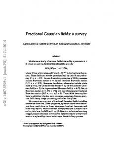
For a positive integer r, let Br be a collection of sub-boxes of side length r which forms a partition of V⌊N/r⌋r . Write B = ∪r∈[N ] Br . Let {gB : B ∈ B} be a collection of i.i.d. standard Gaussian variables. For v ∈ VN , denote by Bv,r ∈ Br the box that contains v. For σ = (σ1 , σ2 ) with kσk22 = σ12 + σ22 and r1 , r2 , define, ϕ˜N,r1 ,r2 ,σ,v = ϕN,v + σ1 gBv,r1 + σ2 gBv,N/r2 ,

(15)

˜ N,r ,r ,σ = maxv∈V ϕ˜N,r ,r ,σ,v . and set M 1 2 1 2 N For probability measures ν1 , ν2 on R, let d(ν1 , ν2 ) denote the L´evy distance between ν1 , ν2 , i.e. d(ν1 , ν2 ) = inf{δ > 0 : ν1 (B) ≤ ν2 (B δ ) + δ

for all open sets B},

where B δ = {y : |x − y| < δ for some x ∈ B}. In addition, define ˜ 1 , ν2 ) = inf{δ > 0 : ν1 ((x, ∞)) ≤ ν2 ((x − δ, ∞)) + δ d(ν

for all x ∈ R} .

˜ 1 , ν2 ) = 0, then ν1 is stochastically dominated by ν2 . Thus, d(ν ˜ 1 , ν2 ) measures approximate If d(ν ˜ ·) is not symmetric. stochastic domination of ν1 by ν2 ; in particular, unlike d(·, ·), the function d(·, With a slight abuse of notation, if X, Y are random variables with laws µX , µY respectively, we ˜ ˜ X , µY ). also write d(X, Y ) for d(µX , µY ) and d(X, Y ) for d(µ A notation convention: By Proposition 1.1, one has that lim sup lim sup d(max ϕN,v , max ϕN,v ) = 0 . δ→0

N

v∈VNδ

v∈VN

Therefore, in order to prove Theorem 1.3, it suffices to show that for each fixed δ > 0, the law of maxv∈V δ ϕN,v − mN converges. To this end, one only needs to consider the Gaussian field restricted N

to VNδ . For convenience of notation, we will treat VNδ as the whole box that is under consideration. Equivalently, throughout the rest of the paper when assuming (A.1), (A.2) or (A.3) holds, we assume these assumptions hold with δ = 0, and we set α := max(α0 , α(0) . The following lemma, which is one of the main results of this section, relates the laws of MN ˜ N,r ,r ,σ . and M 1 2 Lemma 3.1. The following holds uniformly for all Gaussian fields {ϕN,v : v ∈ VN } satisfying Assumption (A.1): p ˜ N,r ,r ,σ − mN − kσk2 d/2) = 0 . (16) lim sup lim sup d(MN − mN , M 1 2 2 r1 ,r2 →∞ N →∞

The next lemma states that under Assumption (A.1), the law of the maximum is robust under small perturbations (in the sense of ℓ∞ norm) of the covariance matrix.

Lemma 3.2. Let {ϕN,v : v ∈ VN } be a sequence of Gaussian fields satisfying Assumption (A.1), and let σ be fixed. Let {ϕ¯N,v : v ∈ VN } be Gaussian fields such that for all u, v ∈ VN | Var ϕN,v − Var ϕ¯N,v | ≤ ǫ, and Eϕ¯N,v ϕ¯N,u ≤ EϕN,v ϕN,u + ǫ . Then, there exists ι = ι(ǫ) with ι →ǫ→0 0 such that ˜ N − mN , max ϕ¯N,v − mN ) ≤ ι . lim sup d(M N →∞

v∈VN

12

gB.,r1 gB.,N/r2 r1

N r2

N Figure 1: Perturbation levels of the Gaussian field

A key step in the proof of Lemma 3.1 is the following characterization of the geometry of vertices achieving large values in the fields, an extension of [11, Theorem 1.1]; it states that near maxima are either at microscopic or macroscopic distance from each other. This may be of independent interest. Lemma 3.3. There exists a constant c > 0 such that, uniformly for all Gaussian fields satisfying Assumption (A.1), we have lim lim P(∃u, v : |u − v| ∈ (r, Nr ), ϕN,v , ϕN,u ≥ mN − c log log r) = 0 .

r→∞ N →∞

3.1

Maximal sum over restricted pairs

As in the case of 2D DGFF discussed in [11], in order to prove Lemma 3.3, we will study the maximum of the sum over restricted pairs. For any Gaussian field {ηN,v : v ∈ VN } and r > 1, define ⋄ ηN,r = max{ηN,u + ηN,v : u, v ∈ VN , r ≤ |u − v| ≤ N/r} .

Lemma 3.4. There exist constants c1 , c2 depending only on d and C > 0 depending only on (α, d) such that for all r, n with N = 2n and all Gaussian fields satisfying Assumption (A.1), we have 2mN − c2 log log r − C ≤ Eϕ⋄N,r ≤ 2mN − c1 log log r + C .

13

(17)

Proof. In order to prove Lemma 3.4, we will show that ES2⋄−κ N,r ≤ Eϕ⋄N,r ≤ ES2⋄κ N,r .

(18)

To this end, we recall the following Sudakov-Fernique inequality [13] which compares the first moments for maxima of two Gaussian processes. Lemma 3.5. Let A be an arbitrary finite index set and let {Xa : a ∈ A} and {Ya : a ∈ A} be two centered Gaussian processes such that: E(Xa − Xb )2 ≥ E(Ya − Yb )2 ,

for all a, b ∈ A .

Then E(maxa∈A Xa ) ≤ E(maxa∈A Ya ). We will give a proof for the upper bound in (17). The proof of the lower bound follows using similar arguments. For κ ∈ N, recall the definition of the restriction map ψN as in (9). By Lemma 2.3, there exists a κ > 0 (depending only on (α, d)) such that for all u, v, u′ , v ′ ∈ VN , κ

κ

κ

κ

E(ϕN,u + ϕN,v − ϕN,u′ − ϕN,v′ )2 ≤ E(Sψ2 NN(u) + Sψ2 NN(v) − Sψ2 NN(u′ ) − Sψ2 NN(v′ ) )2 . κ

κ

(To see this, note that the variance of Sψ2 NN(u) increases with κ but the covariance between Sψ2 NN(u) and κ Sψ2 NN(v) does not.) In addition, note that for r ≤ |u−v| ≤ N/r one has r ≤ |ψN (u)−ψN (v)| ≤ 2κ N/r. Combined with Lemma 3.5, this yields Eϕ⋄N,r ≤ ES2⋄κ N,r , completing the proof of the upper bound in (18). To complete the proof of Lemma 3.5, note that [11, Lemma 3.1] readily extends to MBRW in d-dimension, and thus ⋄ 2mN − c2 log log r − C ≤ ESN,r ≤ 2mN − c1 log log r + C ,

where c1 , c2 are constants depending only on d and C is a constant depending on (α, d). Combined with (18), this completes the proof of the lemma. We will also need the following tightness result. Lemma 3.6. Under Assumption (A.1), the sequence {(ϕ⋄N,r − Eϕ⋄N,r )/ log log r}N ∈N,r≥100 is tight. Further, there exists a constant C > 0 depending only on d such that for all r ≥ 100 and N ∈ N, |(ϕ⋄N,r − Eϕ⋄N,r )| ≤ C log log r . (1)

(2d )

Proof. Take N ′ = 2N and partition VN ′ into 2d copies of VN , denoted by VN , . . . , VN . For each (i) (i) i ∈ [2d ], let {ϕN,v : v ∈ VN } be an independent copy of {ϕN,v : v ∈ Vn } where we identify VN and (i)

VN by the suitable translation such that the two boxes coincide. Denote by (i)

(i)

ϕˆN ′ ,v = ϕN,v for v ∈ VN and i ∈ [2d ] .

(19)

Clearly, {ϕN ′ ,v } is a Gaussian field that satisfies Assumption (A.1) (with α increased by an absolute constant). Therefore, by Lemma 3.4, we have 2mN − c2 log log r − C ≤ Eϕˆ⋄N,r ≤ 2mN − c1 log log r + C , 14

(20)

where c1 , c2 , C > 0 are constants depending only on (d, α). In addition, we have (1),⋄

(2),⋄

E(ϕˆ⋄N ′ ,r ) ≥ E max{ϕN,r , ϕN,r } . Combined with Lemma 3.4 and (20), and the simple algebraic fact that |a − b| = 2(a ∨ b) − a − b, it yields that (1),⋄

(2),⋄

E|ϕN,r − ϕN,r | ≤ 2(Eϕˆ⋄N ′ ,r − Eϕ⋄N,r ) ≤ C ′ log log r , for all r ≥ 100 , where C ′ > 0 is a constant depending only on d. This completes the proof of the lemma.

3.2

Proof of Lemma 3.3

In this subsection we will prove Lemma 3.3, by contradiction. Suppose otherwise that Lemma 3.3 does not hold. Then for any constant c > 0, there exists ǫ > 0 and a subsequence {rk } such that for all k ∈ N  
N (21) , ϕN,v , ϕN,u ≥ mN − c log log rk > ǫ . lim P ∃u, v : |u − v| ∈ rk , N →∞ rk

Now fix δ > 0 and consider N ′ = 2κ N where κ is an integer to be selected. Partition VN ′ into 2κd (2κd ) (1) disjoint boxes of side length N , denoted by VN , . . . , VN . Define {ϕˆN ′ ,v : v ∈ VN ′ } in the same (i) manner as in (19) except that now we take 2κd copies of {ϕN,v : v ∈ VN } (one for each VN with i ∈ [2κd ]). Clearly, {ϕˆN ′ ,v : v ∈ VN ′ } is a Gaussian field satisfies Assumption (A.1) with α replaced by a constant α′ depending only on (α, d, κ). Therefore, by Lemma 3.4, 2mN − c2 log log r − C ≤ Eϕˆ⋄N ′ ,r ≤ 2mN − c1 log log r + C ,

(22)

where c1 , c2 > 0 are two constants depending only on d and C > 0 is a constant depending only on (α, d, κ). Next we derive a contradiction to (22). Set zN,r = 2mN − c log log r, ZN,r = (ϕˆ⋄N ′ ,r − zN,r )− (i)

(i),⋄

and YN,r = (ϕN,rk − zN,r )− . Then (21) implies that (1)

lim P(YN,rk > 0) ≤ 1 − ǫ for all k ∈ N .

N →∞

(23)

In addition, by Lemmas 3.4 and 3.6, there exists a constant C ′ > 0 depending only on d such that for all r ≥ 100 and N ∈ N, we have (1)

EYN,r ≤ C ′ log log r . (i)

(24) (i)

Clearly, ZN,r ≤ mini∈[2κd ] YN,r . Combined with the fact that YN,r are i.i.d. random variables, one obtains Z ∞ Z ∞ κd (1) (1) (1) 2κd −1 2κd (P(YN,rk > y)) dy ≤ (1 − ǫ) EZN,rk ≤ (P(YN,rk > y))dy ≤ (1 − ǫ)2 −1 EYN,rk , 0

0

where (23) was used in the second inequality. Combined with (24), one concludes that for all r ≥ 100 and N κd EZN,rk ≤ (1 − ǫ)2 −1 C ′ log log rk . 15

κd −1

Now set c = c1 /4 and choose κ depending on (ǫ, d, C ′ , c1 ) such that (1 − ǫ)2

C ′ ≤ c1 /4. Then,

Eϕˆ⋄N ′ ,rk ≥ 2mN − c1 log log rk /2 , for all k ∈ N and sufficiently large N ≥ Nk where Nk is a number depending only on k. Sending N → ∞ first and then k → ∞ contradicts (22), thereby completing the proof of the lemma.

3.3

Proof of Lemmas 3.1 and 3.2

The next lemma, which extends [7, Lemma 3.9] to the current setup, will be useful for the proof of Lemma 3.1 and later in the paper. Lemma 3.7. Let Assumptions (A.0) and (A.1) holds. Let {φN u : u ∈ VN } be a collection of random variables independent of {ϕN,u : u ∈ VN } such that 2

−y for all u ∈ VN . P(φN u ≥ 1 + y) ≤ e

(25)

Then, there exists C = C(α, d) > 0 such that, for any ǫ > 0, N ∈ N and x ≥ −ǫ−1/2 , P(max (ϕN,u + ǫφN u ) ≥ mN + x) ≤ P(max ϕN,u ≥ mN + x − u∈VN

u∈VN

√

ǫ)(1 + C(e−C

−1 ǫ−1

)) .

(26)

Proof. We first give the proof for ǫ ≤ 1. Define Γy = {u ∈ VN : y/2 ≤ ǫφN u ≤ y}. Then, √ P(max (ϕN,u + ǫφN u ) ≥ mN + x) ≤P(MN ≥ mN + x − ǫ) u∈VN

+

∞ X i=0

√ E(P( max ϕN,u ≥ mN + x − 2i ǫ|Γ2i √ǫ )) . u∈Γ2i √ǫ

By Proposition 1.1, one can bound the second term on the right hand side above by ∞ X

∞ √ √ √ x∨1 X i E(P(max ϕN,u ≥ mN + x − 2i ǫ|Γ2i √ǫ )) . √ E(|Γ2i √ǫ |/N d )1/2 e 2d2 ǫ . u∈VN e 2dx i=0 i=0 i

−1

By (25), one has E(|Γ2i √ǫ |/N d )1/2 ≤ e−4 (Cǫ) . Altogether, one gets ∞ X

√ x∨1 −1 E(P(max ϕN,u ≥ mN + x − 2i ǫ|Γ2i √ǫ )) . √ e−(Cǫ) , u∈VN e 2dx i=0

completing the proof of the lemma when ǫ ≤ 1. The case ǫ > 1 is simpler and follows by repeating the same argument with Γ2i ǫ replacing Γ2i √ǫ . We omit further details. We next consider a combination of two independent copies of {ϕN,v }. For σ > 0, define s kσk22 ′ ∗ ϕ for v ∈ VN , and MN,σ = max ϕ∗N,σ,v . ϕ∗N,σ,v = ϕN,v + v∈VN log N N,v

(27)

where {ϕ′N,v : v ∈ VN } is an independent copy of {ϕN,v : v ∈ VN }. Note that the field {ϕ∗N,σ,v } is p distributed like the field {aN ϕN,v } where aN = 1 + kσk22 / log N . 16

Remark 3.8. The idea of writing a Gaussian field as a sum of two independent Gaussian fields has been extensively employed in the study of Gaussian processes. In the context of the study of extrema of the 2D DGFF, this idea was first used in [3], where (combined with an invariance result from [18] as well as the geometry of the maxima of DGFF [11], see Lemma 3.4) it led to a complete description of the extremal process of 2D DGFF. The definition (27) is inspired by [3]. The following is the key to the proof of Lemma 3.1. Proposition 3.9. Let Assumption (A.1) hold. Let {ϕ˜N,r,σ,v : v ∈ VN } and {ϕ∗N,σ,v : v ∈ VN } be defined as in (15) and (27) respectively. Then for any fixed σ, lim

˜ N,r ,r ,σ − mN , M ∗ − mN ) = 0 . lim sup d(M 1 2 N,σ

r1 ,r2 →∞ N →∞

(28)

Proof. Partition VN into boxes of side length N/r2 and denote by B the collection of boxes. Fix an arbitrary small δ > 0, and let Bδ denote the box in the center of B with side length (1 − δ)N/r2 ˜ N,r ,r ,σ,δ = maxv∈V ϕ˜N,r ,r ,σ,v and M ∗ for each B ∈ B. Write VN,δ = ∪B∈B Bδ . Set M 1 2 1 2 N,δ N,σ,δ = ∗ maxv∈VN,δ ϕN,σ,v . By (3), one has ∗ ˜ N,r ,r ,σ,δ 6= M ˜ N,r ,r ,σ ) = lim lim P(M ∗ lim lim P(M 1 2 N,σ,δ 6= MN,σ ) = 0 . 1 2

δ→0 N →∞

δ→0 N →∞

∗ ˜ ˜ N,r ,r ,σ,δ and M ∗ Therefore, it suffices to prove (28) with M 1 2 N,σ,δ replacing MN,r1 ,r2 ,σ and MN,σ . To this end, let zB be such that

max ϕN,v = ϕN,zB for every B ∈ B .

v∈Bδ

We will show below that lim

˜ N,r ,r ,σ,δ − max ϕ˜N,r ,r ,σ,z | ≥ 1/ log log N ) lim sup P(|M 1 2 1 2 B

r1 ,r2 →∞ N →∞ ∗ = lim sup P(|MN,σ,δ N →∞

B∈B

− max ϕ∗N,σ,zB | ≥ 1/ log log N ) = 0 . B∈B

(29)

p Note that conditioning on the field {ϕN,v : v ∈ VN }, the field { kσk22 /log N ϕ′N,v : B ∈ B} is centered Gaussian fieldqwith pairwise correlation bounded by O(1/ log N ). Therefore the conditional kσk2

covariance matrix of { log N2 ϕ′N,zB : B ∈ B} and that of {σ1 gBzB ,r1 +σ2 gBzB ,N/r2 : B ∈ B} are within additive O(1/ log N ) of each other entrywise. Combined with (29), it then yields the proposition. It remains to prove (29). Write r = r1 ∧ r2 and let C be a constant which we will send to infinity after sending first N → ∞ and then r → ∞, and let c be the constant from Lemma 3.3. Suppose that either of the events that are considered in (29) occurs. In this case, one of the following events has to occur: ˜ N,r ,r ,σ,δ 6∈ (mN − C, mN + C)} ∪ {M ∗ • The event E1 = {M 1 2 N,σ,δ 6∈ (mN − C, mN + C)}. • The event E2 that there exists u, v ∈ (r, N/r) such that ϕN,u ∧ ϕN,v > mN − c log log r. ˜ N,r ,r ,σ (M ∗ ) is achieved at a ˜3 (E ∗ ) is the event that M ˜3 ∪ E ∗ where E • The event E3 = E 1 2 3 3 N,σ,δ vertex v such that ϕN,v ≤ mN − c log log r. 17

• The event E4 that there exists v ∈ B ∈ B with ϕN,v ≥ mN − c log log r and r r kσk22 ′ log N ϕN,v

−

kσk22 ′ log N ϕN,zB

≥

1 log log N

.

By Theorem 1.2, limC→∞ lim supN →∞ P(E1 ) = 0. By Lemma 3.3, limr→∞ lim supN →∞ P(E2 ) = 0. In addition, writting Γx = {v ∈ VN : ϕ˜N,r1 ,r2 ,σ,v − ϕN,v ∈ (x, x + 1)}, one has ˜3 ) ≤ P( P(E1c ∩ E

max X

max ϕ˜N,r1 ,r2 ,σ,v ≥ mN − C)

x≥c log log r−C v∈Γx

≤ ≤

x≥c log log r−C

X

x≥c log log r−C

X

.C

P(max ϕ˜N,r1 ,r2 ,σ,v ≥ mN − C) v∈Γx

E(P(max ϕN,v ≥ mN − x − C|Γx )) v∈Γx

√

x≥c log log r−C

E(|Γx |/N d )1/2 xe

2dx

,

where the last inequality follows from (3). From simple estimates using the Gaussian distribution ′ 2 one has E(|Γx |/N d )1/2 ≤ e−c x /c′ where c′ = c′ (σ) > 0. Therefore, one concludes that ˜3 ) = 0 . lim sup lim sup lim sup P(E1c ∩ E r→∞

C→∞

N →∞

A similar argument leads to the same estimate with E3∗ replacing E3 . Thus, lim sup lim sup lim sup P(E1c ∩ E3 ) = 0 . r→∞

C→∞

N →∞

Finally, let Γ′r = {v : ϕN,v ≥ mN − c log log r}. On the event E2c , one has |Γ′r | ≤ r 4 . Further, for each v ∈ B ∩ Γ′r , on E2c one has |v − zB | ≤ r and thus (by the independence between {ϕN,v } and {ϕ′N,v }), r r P(

kσk22 ′ log N ϕN,v

−

kσk22 ′ log N ϕN,zB

≥ 1/ log log N ) = oN (1) .

Therefore, a union bound gives that

lim sup lim sup P(E4 ∩ E2c ) ≤ lim sup lim sup r 4 oN (1) = 0 . r→∞

r→∞

N →∞

N →∞

Altogether, this completes the proof of (29) and hence of the proposition. Proof of Lemma 3.1. Define   kσk22 ¯ N,σ = max ϕ¯N,v . ϕ¯N,σ,v = 1 + ϕN,v for v ∈ VN , and M v∈VN 2 log N 2

¯ N,σ = (1 + kσk2 )MN . Combined with (1), it gives that EM ¯ N,σ = EMN + Clearly we have M 2 log N p 2 ¯ N,σ − EM ¯ N,σ ) → 0 as N → ∞. Further define {ϕ∗ σ d/2 + o(1) and that d(MN − EMN , M N,σ,v : ∗ v ∈ VN } as in (27). By the fact that the field {ϕ¯N,σ,v } can be seen as a sum of {ϕN,σ,v } and ¯ N,σ = an independent field whose variances are O((1/ log N )3 ) across the field, we see that EM ∗ EMN,σ + o(1) and that ∗ ∗ ¯ N,σ − EM ¯ N , MN,σ d(M − EMN ) → 0. (30) Combined with Proposition 3.9, this completes the proof of the lemma. 18

Proof of Lemma 3.2. Let φ and φN,v be i.i.d. standard Gaussian variables, and for ǫ∗ > 0 let ϕlw,N,ǫ∗ ,v = (1 − ǫ∗ / log N )ϕN,v + ǫ′N,v φ and ϕ¯up,N,ǫ∗ ,v = (1 − ǫ∗ / log N )ϕ¯N,v + ǫ′′N,v φN,v , where ǫ′N,v , ǫ′′N,v are chosen so that Var ϕlw,N,ǫ∗ ,v = Var ϕ¯up,N,ǫ∗ ,v = Var ϕN,v + ǫ. We can choose ǫ∗ = ǫ∗ (ǫ) with ǫ∗ →ǫ→0 0 so that Eϕlw,N,ǫ∗ ,v ϕlw,N,ǫ∗ ,u ≥ Eϕ¯up,N,ǫ∗ ,v ϕ¯up,N,ǫ∗ ,u for all u, v ∈ VN . By Lemma 2.4, one has ˜ d(max ϕlw,N,ǫ∗ ,v − mN , max ϕ¯up,N,ǫ∗,v − mN ) = 0 . v∈VN

v∈VN

Combined with Lemma 3.7, this completes the proof of the lemma.

4

Proofs of Theorems 1.3 and 1.4

In this section we assume (A.0)–(A.3) and prove Theorem 1.3. Toward this end, in Subsection 4.1 we will approximate the field {ϕN,v : v ∈ VN } by a simpler to analyze field, in such a way that the results of Section 3 apply and yield the asymptotic equivalence of their respective laws of the centered maximum. In Subsection 4.2 we prove the convergence in law for the centered maximum of the new field. Our method of proof yields Theorem 1.4 as a byproduct.

4.1

An approximation of the log-correlated Gaussian field

In this subsection, we approximate the log-correlated Gaussian field. Let RN (u, v) = E(ϕN,u ϕN,v ). We consider three scales for the approximation of the field {ϕN,v }: (a) The top (macroscopic) scale, dealing with RN (u, v) for |u − v| ≍ N . (b) The bottom (microscopic) scale, dealing with RN (u, v) for |u − v| ≍ 1. (c) The middle (mesoscopic) scale, dealing with RN (u, v) for 1 ≪ |u − v| ≪ N . By Assumptions (A.2) and (A.3), RN (u, v), properly centered, converges in the top and bottom scale. So in those scales, we approximate {ϕN,u } by the corresponding “limiting” fields. In the middle scale, we simply approximate {ϕN,u } by the MBRW. One then expects that this approximation gives an additive o(1) error for RN (u, v) in the top and bottom scale, and an additive O(1) error in the middle scale. It turns out that this guarantees that the limiting laws of the centered maxima coincide. In what follows, for any integer t we refer to a box of side length t as an t-box. Take two large integers L = 2ℓ and K = 2k . Consider first {ϕKL,u : u ∈ VKL } in a KL-box whose left-bottom corner is identified as the origin, and let Σ denote its covariance matrix. Recall that by Proposition 1.1, with probability tending to 1 as N → ∞, the maximum of ϕN,v over VN occurs in a sub-box of VN with side length ⌊N/KL⌋ · KL. Therefore, one may neglect the maximization over the indices in VN \ V⌊N/KL⌋·KL . For notational convenience, we will assume throughout that KL divides N in what follows. We use Σ to approximate the macroscopic scale of RN (u, v), as follows. Partition VN into a disjoint union of boxes of side length N/KL, denoted BN/KL = {BN/KL,i : i = 1, . . . , (KL)d }. Let vN/KL,i . Let Ξc be a matrix of vN/KL,i be the left bottom corner of box BN/KL,i and write wi = N/KL 19

dimension N d × N d such that Ξcu,v = Σwi ,wj for u ∈ BN/KL,i and v ∈ BN/KL,j . Note that Ξc is a positive definite matrix with diagonal terms log(KL) + OKL (1). ′ ′ Next, take two other integers K ′ = 2k and L′ = 2ℓ . As above, we assume that K ′ L′ divides N . Consider {ϕK ′ L′ ,u : u ∈ VK ′ L′ } in a K ′ L′ -box whose left-bottom corner is identified as the origin, and denote by Σ′ the covariance matrix for {ϕK ′ L′ ,u : u ∈ VK ′ L′ }. As above, assume for notational convenience that K ′ L′ divides N . Partition VN into a disjoint union of boxes of side length K ′ L′ , denoted BK ′ L′ = {BK ′ L′ ,i : i = 1, . . . , (N/K ′ L′ )d }. Let vK ′ L′ ,i be the left bottom corner of BK ′ L′ ,i . Let Ξb be a matrix of dimension N d × N d so that ( Σ′u−vK ′ L′ ,i ,v−vK ′ L′ ,i , u, v ∈ BK ′ L′ ,i Ξbu,v = . 0, u ∈ BK ′ L′ ,i , v ∈ BK ′ L′ ,j , i 6= j Note that Ξb is a positive definite matrix with diagonal terms log(K ′ L′ ) + OK ′ L′ (1). c Let {ξN,v : v ∈ VN } be a Gaussian field with covariance matrix Ξc , which we occasionally refer b to as the coarse field, and let {ξN,v : v ∈ VN } be a Gaussian field with covariance matrix Ξb , which we occasionally refer to as the bottom field. Note that the coarse field is constant in each box BN/KL,i , and the bottom fields in different boxes BK ′ L′ ,i are independent of each other. We will consider the limits when L, K, L′ , K ′ are sent to infinity in that order. In what follows, we denote by (L, K, L′ , K ′ ) ⇒ ∞ sending these parameters to infinity in the order of K ′ , L′ , K, L (so K ′ ≫ L′ ≫ K ≫ L). K ′ L′

··· ··· N/(KL)

c ξN,·

b ξN,· independent between K ′ L′ boxes

correlated constant inside N/(KL) boxes K ′ L′

ξN,·,M BRW independent between N/(KL) boxes

N Figure 2: Hierarchy of construction of the approximating Gaussian field Finally, we give the MBRW approximation for the mesoscopic scales. Recall the definitions of BjN and Bj (v) in Subsection 2.1, and recall that {bi,k,B : k ≥ 0, 1 ≤ i ≤ (KL)d , B ∈ BkN } is 20

a family of independent Gaussian variables such that Var bi,j,B = log 2 · 2−dj for all B ∈ BjN and 1 ≤ i ≤ (KL)d . For v ∈ BN/KL,i ∩ BK ′ L′ ,i′ (where i = 1, . . . , (KL)d and i′ = 1, . . . , (N/K ′ L′ )d ), define n−k−ℓ X X bN (31) ξN,v,MBRW = i,j,B . j=ℓ′ +k ′ B∈Bj (vK ′ L′ ,i′ )

Note that by our construction {ξN,v,MBRW : v ∈ BN/KL,i } are independent of each other for c i = 1, . . . , (KL)d , and in addition ξN,·,MBRW is constant over each K ′ L′ -box. Further, let {ξN,v : b v ∈ VN }, {ξN,v : v ∈ VN } and {ξN,v,MBRW : v ∈ VN } be independent of each other. One has by Assumption (A.1) that c b | Var(ξN,v + ξN,v + ξN,v,MBRW ) − Var ϕN,v | ≤ 4α .

Let aN,v be a sequence of numbers such that for all v ∈ BN/KL,i and all 1 ≤ i ≤ (KL)d , c b Var(ξN,v + ξN,v + ξN,v,MBRW ) + a2N,v = Var ϕN,v + 4α .

(Here, the sequence aN,v implicitly depends on (KL).) It is clear that √ max aN,v ≤ 8α . v∈VN

(32)

(33)

For v ∈ BN/KL,i and v ≡ v¯ mod K ′ L′ , one has N a2N,v = Var ϕN,v + 4α − Var ϕKL,wi − Var ϕK ′ L′ ,¯v − log( KLK ′ L′ )

N = log N − log(KL) + ǫN,KL,K ′L′ + 4α − Var ϕK ′ L′ ,¯v − log( KLK ′ L′ ) ≥ 0,

where, by Assumptions (A.2), lim sup ǫN,KL,K ′L′ = 0 .

lim sup

(34)

(L,K,L′ ,K ′ )⇒∞ N →∞

Therefore, one can write a2N,v = a2K ′ ,L′ ,¯v + ǫN,KL,K ′L′ , where aK ′ L′ ,¯v depends on

(K ′ L′ , v¯).

lim sup (L,K,L′ ,K ′ )⇒∞

(35)

By Assumption (A.2) and the continuity of f , one has sup

u,v:ku−vk∞

≤L′

b b lim sup | Var ξN,v − Var ξN,u | = 0. N →∞

Therefore, we can further require that v−u ¯k∞ ≤ L′ . |aK ′ L′ ,¯v − aK ′ L′ ,¯u | ≤ ǫN,KL,K ′L′ for all k¯

(36)

Let φj be i.i.d. standard Gaussian variables. For v ∈ BK ′ L′ ,j and v ≡ v¯ mod K ′ L′ , define c b ξN,v = ξN,v + ξN,v + ξN,v,MBRW + aK ′ L′ ,¯v φj .

(37)

It follows from (32) and (35) that lim sup

lim sup | Var ξN,v − Var ϕN,v − 4α| = 0 .

(L,K,L′ ,K ′ )⇒∞ N →∞

21

(38)

Finally, we partition VN into a disjoint union of boxes of side length N/L which we denote by BN/L = {BN/L,i : 1 ≤ i ≤ Ld }, as well as a disjoint union of boxes of side length L which we denote by BL = {BL,i : 1 ≤ i ≤ (N/L)d }. Again, we denote by vN/L,i and vL,i the left bottom corner of the boxes BN/L,i and BL,i , respectively. For δ > 0 and any box B, denote by B δ ⊆ B the collection of all vertices in B that are δℓB away from its boundary ∂B (here ℓB is the side length of B). Let ∗ δ δ δ VN,δ = (∪i BN/L,i ) ∩ (∪i BN/KL,i ) ∩ (∪i BL,i ) ∩ (∪i BKL,i ) . ∗ | ≥ (1 − 100dδ)|V |. One has |VN,δ N The following lemma suggests that {ξN,v : v ∈ VN } is a good approximation of {ϕN,v : v ∈ VN }.

Lemma 4.1. Let Assumptions (A.1), (A.2) and (A.3) hold. Then there exist ǫ′N,K,L,K ′,L′ > 0 with ∗ : lim sup(L,K,L′ ,K ′ )⇒∞ lim supN →∞ ǫ′N,K,L,K ′,L′ = 0 , such that the following hold for all u, v ∈ VN,δ (a) If u, v ∈ BL′ ,i for some 1 ≤ i ≤ (N/L′ )d , then |E(ξN,u − ξN,v )2 − E(ϕN,u − ϕN,v )2 | ≤ ǫ′N,K,L,K ′,L′ . (b) If u ∈ BN/L,i , v ∈ BN/L,j with i 6= j, then |EξN,u ξN,v − EϕN,v ϕN,u | ≤ ǫ′N,K,L,K ′,L′ . (c) Otherwise, |EξN,u ξN,v − EϕN,v ϕN,u | ≤ 4 log(1/δ) + 40α. Proof. (a): Let i′ be such that BL′ ,i ⊆ BK ′ L′ ,i′ . By (36) and (37), one has |E(ξN,u − ξN,v )2 − E(ϕKL,u−vKL,i′ − ϕKL,v−vKL,i′ )2 | ≤ 4ǫN,KL,K ′ L′ , where ǫN,KL,K ′L′ satisfies (34) (and was defined therein). By Assumption (A.2), one has lim sup

lim sup |E(ϕKL,u−vKL,i′ − ϕKL,v−vKL,i′ )2 − E(ϕN,u − ϕN,v )2 | = 0 .

(L,K,L′ ,K ′ )⇒∞ N →∞

Altogether, this completes the proof for (a). (b): Let i′ , j ′ be such that u ∈ BN/KL,i′ and v ∈ BN/KL,j ′ , and assume w.l.o.g. that K ′ ≫ L′ ≫ K ≫ L ≫ 1/δ. The definition of {ξN,v } gives EξN,v ξN,u = EϕKL,wi′ ϕKL,wj′ v

′

v

′

N/KL,j ′ ′ ′ where wi′ = N/KL,i N/KL and wj = N/KL . In this case, we have |wi − wj | ≥ δK. Writing xu = u/N, xv = v/N and yu = wi′ /KL, yv = wj ′ /KL, one obtains

|yu − yv | ≥ δ/L, |xu − xv | ≥ δ/L, |xu − yu | ≤ 1/K, |xv − yv | ≤ 1/K . Therefore, Assumption (A.3) yields lim sup(L,K,L′ ,K ′ )⇒∞ lim supN →∞ |EξN,u ξN,v − EϕN,v ϕN,u | = 0, completing the proof of (b). (c). In this case, one has c c b b EξN,v ξN,u =EξN,v ξN,u + EξN,v ξN,u + EξN,u,MBRW ξN,v,MBRW + err1 |u−v| ) = log KL − log+ ( N/KL

+ 1|u−v|≤N/KL (log

N (KLK ′ L′ )

− log+

|u−v| K ′ L′ ) +

err2

= log N − log+ |u − v| + err2 , where |err1 | ≤ 8α and |err2 | ≤ 2 log 1/δ + 20α. Combined with Assumption (A.1), this completes the proof of (c) and hence of the lemma. 22

Lemma 4.2. Let Assumptions (A.0), (A.1), (A.2) and (A.3) hold. Then, √ lim sup lim sup d(MN − mN , max ξN,v − mN − 2α 2d) = 0 . v∈VN

(L,K,L′ ,K ′ )⇒∞ N →∞

Proof. By Proposition 1.1, it suffices to show that for all δ > 0 √ ξ − m − 2α ϕ − m , max lim sup lim sup d( max 2d) = 0 . N,v N N,v N ∗ ∗

lim sup

(L,K,L′ ,K ′ )⇒∞ N →∞

v∈VN,δ

v∈VN,δ

N →∞

p Consider a fixed δ > 0. Let σ∗2 = 4 log(1/δ) + 60α. Let σlw = (0, σ∗2 + 4α) and σup = (σ ∗ , 0). Define {ϕ˜N,L′ ,L,σlw ,v : v ∈ VN } as in (15) with r1 = L′ , r2 = L and σ = σlw . Analogously, define ∗ , {ξ˜N,L′ ,L,σup ,v : v ∈ VN }. By (37) and Lemma 4.1, one has for all u, v ∈ VN,δ | Var ϕ˜N,L′ ,L,σlw ,v − Var ξ˜N,L′ ,L,σup ,v | ≤ ¯ǫN,K,L,K ′,L′ , Eξ˜N,L,σ ,v ξ˜N,L,σ ,u ≤ Eϕ˜N,L,σ ,v ϕ˜N,L,σ up

up

lw

lw ,u

+ ǫ¯N,K,L,K ′,L′ ,

∗ } satisfies where lim sup(L,K,L′ ,K ′ )⇒∞ lim supN →∞ ǫ¯N,K,L,K ′,L′ = 0. Since {ϕ˜N,L′ ,L,σlw ,v : v ∈ VN,δ Assumption (A.1) with α being replaced by 10α + σ∗2 , one may apply Lemma 3.2 and obtain that

lim sup

˜ max ϕ˜N,L′ ,L,σ ,v − mN , max ξ˜N,L′ ,L,σ ,v − mN ) = 0 . lim sup d( up lw ∗ ∗

(L,K,L′ ,K ′ )⇒∞ N →∞

v∈VN,δ

v∈VN,δ

∗ ), one gets By Lemma 3.1 (it is clear that the same statement holds for maximum over VN,δ p 2 ′ ,L,σ ,v − mN − (σ + 4α) d/2, max ϕN,v − mN ) = 0 , ϕ ˜ lim sup lim sup d( max N,L ∗ lw ∗ v∈VN,δ∗

v∈VN,δ

(L,K,L′ ,K ′ )⇒∞ N →∞

p ξ˜N,L′ ,L,σup ,v − mN − (σ∗2 ) d/2, max ξN,v − mN ) = 0 . lim sup d( max ∗

lim sup

v∈VN,δ∗

v∈VN,δ

(L,K,L′ ,K ′ )⇒∞ N →∞

Altogether, this gives that lim sup

√ ˜ max ϕN,v − mN , max ξN,v − mN − 2α 2d) = 0 . lim sup d( ∗ ∗

(L,K,L′ ,K ′ )⇒∞ N →∞

v∈VN,δ

v∈VN,δ

The other direction of stochastic domination follows in the same manner. Altogether, this completes the proof of the lemma.

4.2

Convergence in law for the centered maximum

In light of Lemma 4.2, in order to prove Theorem 1.3 it remains to show the convergence in law for the centered maximum of {ξN,v : v ∈ VN }. To this end, we will follow the proof of the convergence f c , in law in the case of the 2D DGFF given in [7]. Let the fine field be defined as ξN,v = ξN,v − ξN,v ′ ′ and note that it implicitly depends on K L . As in [7], a key step in the proof of convergence of the centered maximum is the following sharp tail estimate on the right tail of the distribution of f maxv∈B ξN,v for B ∈ BN/KL . The proof of this estimate is postponed to the appendix. Proposition 4.3. Let Assumptions (A.1), (A.2) and (A.3) hold. Then there exist constants ∗ Cα , cα > 0 depending only on α and constansts cα ≤ βK ′ ,L′ ≤ Cα such that √

lim lim sup lim sup lim sup |z −1 e

z→∞ L′ →∞

K ′ →∞

N →∞

2dz

max ξ f v∈BN/KL,i N,v

P(

23

∗ ≥ mN/KL + z) − βK ′ ,L′ | = 0.

(39)

Remark 4.4. Proposition 4.3 is analogous to [7, Proposition 4.1], but there are two important differences: ′ ′ ∗ (a) In Proposition 4.3 the convergence is to a constant βK ′ ,L′ which depends on K , L , while in [7, Proposition 4.1] the convergence is to an absolute constant α∗ . This is because the fine field ξN,v here implicitly depends on K ′ , L′ , and thus a priori one is not able to eliminate the dependence on (K ′ , L′ ) from the limit. However, in the same spirit as in [7], the dependence on (K ′ , L′ ) is not an issue for deducing a convergence in law — the crucial requirement is ′ ′ ∗ the independence of N . Eventually, we will deduce the convergence of βK ′ ,L′ as K , L → ∞ in that order from the convergence in law of the centered maximum.

(b) In [7, Proposition 4.1], one also controls the limiting distribution of the location of the maximizer while in Proposition 4.3 this is not mentioned. This is because in the current situation c } is constant over each box B and unlike the construction in [7], the coarse field {ξN,v N/KL,i , and thus the location of the maximizer of the fine field in each of the boxes BN/KL,i is irrelevant to the value of the maximum for {ξN,v }. Next, we construct the limiting law of the centered maximum of {ξN,v : v ∈ VN }. We partition ∗ [0, 1]d into R = (KL)d disjoint boxes of equal sizes. Let βK ′ ,L′ be as defined in the statement of Proposition 4.3. By that proposition, there exists a function γ : R 7→ R that grows to infinity arbitrarily slowly (in particular, we may assume that γ(x) ≤ log log log x) such that lim lim sup lim sup lim sup ′

z →∞ L′ →∞

K ′ →∞

sup

N →∞ z ′ ≤z≤γ(K ′ L′ )

√

|z −1 e

2dz

max ξ f v∈BN/KL,i N,v

P(

∗ ≥ mN/KL + z) − βK ′ ,L′ | = 0.

Let {̺R,i }R i=1 be independent Bernoulli random variables with ∗ − P(̺R,i = 1) = βK ′ ,L′ γ(KL)e

√

2dγ(KL)

.

In addition, consider independent random variables {YR,i }R i=1 such that P(YR,i > x) =

√ γ(KL)+x − 2dx e γ(KL)

x > 0.

(40)

Let {ZR,i : 1 ≤ i ≤ R} be an independent Gaussian field with covariance matrix Σ (recall that Σ is of dimension R × R). We then define √ max GR,i where GR,i = ̺R,i (YR,i + γ(KL)) + ZR,i − 2d log(KL) G∗K,L,K ′ ,L′ = 1≤i≤R,̺R,i =1

(here we use the convention that max ∅ = 0). Let µ ¯K,L,K ′,L′ be the distribution of G∗K,L,K ′ ,L′ . We note that µ ¯K,L,K ′,L′ does not depend on N . Theorem 4.5. Let Assumptions (A.0), (A.1), (A.2) and (A.3) hold. Then, lim sup

lim sup d(µN , µ ¯K,L,K ′,L′ ) = 0,

(L,K,L′ ,K ′ )⇒∞ N →∞

where µN is the law of maxv∈VN ξN,v − mN . (Note that µN does depend on KL, K ′ L′ .) 24

(41)

Proof of Theorem 1.3. Theorem 1.3 follows from Lemma 4.2 and Theorem 4.5. Next, we give the proof of Theorem 4.5. Our proof is conceptually simpler than that of its analogue [7, Theorem 2.4], since our coarse field is constant over a box of size N/KL (and thus no consideration of the location for the maximizer in the fine field is needed). Proof of Theorem 4.5. Denote by τ = arg maxv∈VN ξN,v . Applying Theorem 1.2 to the Gaussian c c fields {ξN,v : v ∈ VN } and {ξN,v : v ∈ VN } (where the maximum of {ξN,v : v ∈ VN } is equivalent to the maximum of a log-correlated Gaussian field in a KL-box), we deduce that lim sup (L,K,L′ ,K ′ )⇒∞

f lim sup P(ξN,τ ≥ mN/KL + γ(KL) + 1) = 1 .

(42)

N →∞

Therefore, in what follows, we assume w.l.o.g. the occurrence of the event √ f N N − √3 log log KL + γ(KL) + 1} . {ξN,τ ≥ 2d log KL 2 2d

f Let E = ∪1≤i≤R {maxv∈BN/KL,i ξN,v ≥ mN/KL + KL + 1}. A simple union bound over i gives that

lim sup

lim sup P(E) = 0 .

(43)

(L,K,L′ ,K ′ )⇒∞ N →∞

Thus in what follows we assume without loss that E does not occur. Analogously, we let E ′ = ∪1≤i≤R {YR,i ≥ KL + 1 − γ(KL)}. We see from the union bound that lim sup

lim sup P(E ′ ) = 0 .

(44)

(L,K,L′ ,K ′ )⇒∞ N →∞

In what follows, we assume without loss that E ′ does not occur. For convenience of notation, we denote by f MN,i =

max ξ f v∈BN/KL,i N,v

− (mN/KL + γ(KL)) .

By Proposition 4.3, there exists ǫ∗ = ǫ∗ (N, K, L, K ′ , L′ ) with lim sup (L,K,L′ ,K ′ )⇒∞

lim sup ǫ∗ (N, K, L, K ′ , L′ ) = 0 , N →∞

such that for some |ǫ⋄ | ≤ ǫ∗ /4 f P(ǫ⋄ ≤ MN,i ≤ KL − γ(KL) + 1) = P(̺R,i = 1, YR,i ≤ KL − γ(KL) + 1) ,

and that for all −1 ≤ t ≤ KL − γ(KL) + 1 f P(̺R,i=1 , YR,i ≤ t − ǫ∗ /2) ≤ P(ǫ⋄ ≤ MN,i ≤ t) ≤ P(̺R,i=1 , YR,i ≤ t + ǫ∗ /2) . f : 1 ≤ i ≤ R} and {̺i , YR,i : 1 ≤ i ≤ R} such that Therefore, there exists a coupling between {MN,i ′ c on the event (E ∪ E ) , f f f ̺R,i = 1, |YR,i − MN,i | ≤ ǫ∗ if MN,i ≥ ǫ∗ , and |YR,i − MN,i | ≤ ǫ∗ if ̺R,i = 1 .

25

(45)

c In addition, it is trivial to couple such that ξN,v = ZR,i for all v ∈ BN/KL,i and 1 ≤ i ≤ R. Also, notice the following simple fact √ lim sup lim sup lim sup(mN − mN/KL − 2d log(KL)) = 0 . L→∞

K→∞

N →∞

Altogether, we conclude that there exists a coupling such that outside an event of probability tending to 0 as N → ∞ and then (L, K, L′ , K ′ ) ⇒ ∞ (c.f. (42), (43), (44)) we have max (ξN,v − mN ) − G∗K,L,K ′ ,L′ ≤ 2ǫ∗ .

v∈VN

Now, let τ ′ = arg max1≤i≤R GR,i . Applying Theorem 1.2 to the Gaussian field {ZR,i } and using the preceding inequality, we see that lim sup

lim sup P(̺R,τ ′ = 1) = 1 .

(46)

(L,K,L′ ,K ′ )⇒∞ N →∞

Combined with (45), this yields that there exists a coupling such that except with probability tending to 0 as N → ∞ and then (L, K, L′ , K ′ ) ⇒ ∞ we have | max (ξN,v − mN ) − G∗K,L,K ′ ,L′ | ≤ 2ǫ∗ . v∈VN

thereby completing the proof of Theorem 4.5. ¯K,L,K ′,L′ . We will Proof of Theorem 1.4. Recall that G∗K,L,K ′ ,L′ is a random variable with law µ c construct random variables ZK,L , measurable with respect to F := σ({ZR,i }), so that µ ¯K,L,K ′,L′ ((−∞, x])

lim sup (L,K,L′ ,K ′ )⇒∞

∗ − −βK ′ ,L′ ZK,L e

√

E(e

2dx

)

=

lim inf

(L,K,L′ ,K ′ )⇒∞

µ ¯K,L,K ′,L′ ((−∞, x]) ∗ − −βK ′ ,L′ ZK,L e

√

E(e

2dx

= 1.

(47)

)

for all x. To demonstrate (47), due to (46), we may and will assume without loss that ̺R,τ ′ = 1. √ Define SR,i := 2d log(KL) − ZR,i . Then, for any real x, ! R Y c ∗ (1 − P(̺R,i YR,i > SR,i + x − γ(KL) | F )) . (48) P(GK,L,K ′,L′ ≤ x) = E i=1

In addition, the union bound gives that lim sup P(D) = 1 where D = { min SR,i ≥ 2γ(KL)} . 1≤i≤R

KL→∞

So in the sequel we assume that D occurs. By the definition of ̺R,i and YR,i , we get that − ∗ P(̺R,i YR,i > SR,i + x − γ(KL) | F c ) = βK ′ ,L′ (SR,i + x)e

√

2d(SR,i +x)

→ 0 as KL → ∞ .

Therefore, − ∗ exp(−(1 + ǫK,L )βK ′ ,L′ SR,i e

√

2d(x+SR,i )

) ≤ P(̺R,i YR,i ≤ SR,i + x − γ(KL) | F c )

∗ − ≤ exp(−(1 − ǫK,L )βK ′ ,L′ SR,i e

26

√ 2d(x+SR,i )

),

(49)

for ǫK,L > 0 with lim sup ǫK,L = 0. PR

KL→∞

√ e− 2dSR,i

(this is the analogue of a derivative martingale, see (4)). SubDefine ZK,L = i=1 SR,i stituting (49) into (48) completes the proof of (47). Now, combining (47) and Theorem 4.5, we see that we necessarily have ∗ ∗ lim sup lim sup |βK ′ ,L′ − β | = 0 K ′ →∞

L′ →∞ on (K ′ , L′ ).

for a number β ∗ that does not depend Plugging the preceding inequality into (47), we deduce that µ ¯K,L,K ′,L′ ((−∞, x]) µ ¯K,L,K ′,L′ ((−∞, x]) √ √ = lim inf = 1. (50) lim sup ∗Z − 2dx ′ ′ −β e (L,K,L ,K )⇒∞ E(e−β ∗ ZK,L e− 2dx ) K,L (L,K,L′ ,K ′ )⇒∞ E(e ) Combining (50) with Theorem 4.5 again, we see that ZK,L converges weakly to a random variable Z as K → ∞ and then L → ∞. Also note that ZK,L depends only on the product KL. Therefore, this implies that ZN converges weakly to a random variable Z. From the tightness of the laws µ ¯K,L,K ′,L′ , it follows that Z > 0 a.s. This completes the proof of Theorem 1.4. Proof of Remark 1.6. Consider two sequences {ϕN,v } and {ϕ˜N,v } that satisfy assumptions (A.0)– (A.3) with the same functions h(x, y) and f (x) but possibly different functions g(u, v), g˜(u, v) and ′ different constants α(δ) , α(δ), and α0 , α′0 . Introduce the corresponding fields c ˜f ξ˜N,KL,K ′L′ = ξ˜N,KL,K ′ L′ + ξ N,KL,K ′L′ ,

f c ξN,KL,K ′L′ = ξN,KL,K ′ L′ + ξ N,KL,K ′L′ ,

see Section 4.1. Set also

f c ξˆN,KL,K ′L′ = ξ˜N,KL,K ′ L′ + ξ N,KL,K ′L′ .

Let νN , ν˜N denote the laws of the centered maxima maxv∈VN ϕN,v − mN , maxv∈VN ϕ˜N,v − m ˜ N , and ˜ ˆ let µN , µ ˜N , µ ˆN denote the laws of the centered maxima of the ξN , ξN , ξN fields. (Recall that the latter depend also on KL, K ′ L′ but we drop that fact from the notation.) By Lemma 4.2, we have lim sup

lim sup (d(µN , νN ) + d(˜ µN , ν˜N )) = 0 .

(51)

(L,K,L′ ,K ′ )⇒∞ N →∞

For s ∈ R, let θs µ denote the shift of a probability measure µ on R, that is θs µ(A) = µ(A + s) for any measurable set A. Recall the construction of µ ¯K,L,K ′,L′ , see Theorem 4.5, and construct ˆK,L,K ′,L′ . Note that, by construction, there exists s = s(KL), bounded similarly µ ˜K,L,K ′,L′ and µ ˜K,L,K ′,L′ . In particular, from Theorem 4.5 we get that uniformly in KL, so that θs µ ˆK,L,K ′,L′ = µ
lim sup lim sup d(µN , µ (52) µN , θ s µ ˆK,L,K ′,L′ ) = 0 . ¯K,L,K ′ ,L′ ) + d(˜ (L,K,L′ ,K ′ )⇒∞ N →∞

From (51) and (52), one can find a sequence L(N ), K(N ), K ′ (N ), L′ (N ) along which the convergence still holds (as N → ∞). Let {ηv,N } and {ˆ ηv,N } denote the fields {ξv,N } and {ξˆv,N } with this choice of parameters, and let µ ¯N and µ ˆN denote the corresponding laws of the maximum. Let µ∞ , µ ˜∞ denote the limits of µN and µ ˜N , which exist by theorem 1.3. From the above considerations we have that µ ¯N → µ∞ and θs(N ) µ ˆN → µ ˜∞ . On the other hand, the fields ηN,· and ηˆN,· both satisfy assumptions (A.0)-(A.3) with the same functions f, g, h and thus, interleaving between then one deduces that the laws of their centered maxima converge to the same limit, denoted Θ∞ . It follows that necessarily, s(N ) converges and µ∞ = θs µ ˜∞ = Θ∞ . Using the characterization in Theorem 1.4, this yields the claim in the remark. 27

5

An example: the circular logarithmic REM

In the important paper [15], the authors introduce a one dimensional logarithmically correlated Gaussian field, which they call the circular logarithmic REM (CLREM). Fyodorov and Bouchaud consider the CLREM as a prototype for Gaussian fields exhibiting Carpentier-LeDoussal freezing. (We do not discuss in this paper the notion of freezing, referring instead to [15] and to [22].) Explicitly, fix an integer N , set θk = 2πk/N , and introduce the matrix    1 2 θk − θℓ 1k6=ℓ + (log N + W )1k=ℓ , Rk,ℓ = − log 4 sin 2 2 where W is a constant independent on N . It is not hard to verify (and this is done explicitly in [15]) that one can choose W so that the matrix R is positive definite for all N ; the resulting Gaussian field ϕN,v with correlation matrix R is the CLERM. One may think of the CLREM as indexed by VN in dimension d = 1, or (as the name indicates) by an equally spaced collection of N points on the unit circle in the complex plane. Let MN = maxv∈VN ϕN,v . The following is a corollary of Theorems 1.2 and 1.4. √ √ Corollary 5.1. EMN = 2 log N − (3/2 2) log log N + O(1) and there exist a constant β ∗ and a random variable Z so that lim P(MN − EMN ≤ x) = E(e−β

N →∞

∗ Ze−

√

2x

).

(53)

Proof. Assumptions (A.0) and (A.1) are immediate to check. An explicit computation reveals that Assumption (A.2) holds with f (x) = 0 and  −W, u=v g(u, v) = . log(4π) + |u − v|, u 6= v Finally, it is clear that Assumption (A.3) holds with h(x, y) = log(4 sin2 (2π|x−y|)). Thus, Theorems 1.3 and 1.4 apply and yields (53). Remark 5.2. Remarkably, in [15] the authors compute explicitly, albeit nonrigorously, the law of the maximum of the CLREM, up to a deterministic shift that they do not compute. It was observed in [22] that the law computed in [15] is in fact the law of a convolutions of two Gumbel random variables. In the notation of Corollary 5.1, this means that one expects that 2−1/2 log(β ∗ Z) is Gumbel distributed. We do not have a rigorous proof for this claim. Acknowledgement Remark 1.6 answers a question posed to us by Vincent Vargas. We thank him for the question and for his insights.

References [1] E. A¨ıd´ekon. Convergence in law of the minimum of a branching random walk. 41(3A):1362–1426, 2013.

Ann. Probab.,

[2] M. Bachmann. Limit theorems for the minimal position in a branching random walk with independent logconcave displacements. Adv. Appl. Prob., 32:159–176, 2000.

28

[3] M. Biskup and O. Louidor. Extreme local extrema of two-dimensional discrete gaussian free field. Preprint, available at http://arxiv.org/abs/1306.2602, 2013. [4] M. Biskup and O. Louidor. Conformal symmetries in the extremal process of two-dimensional discrete gaussian free field. Preprint, available at http://arxiv.org/abs/1410.4676, 2014. [5] M. Bramson. Maximal displacement of branching Brownian motion. 31(5):531–581, 1978.

Comm. Pure Appl. Math.,

[6] M. Bramson. Convergence of solutions of the Kolmogorov equation to travelling waves. Mem. Amer. Math. Soc., 44(285):iv+190, 1983. [7] M. Bramson, J. Ding, and O. Zeitouni. Convergence in law of the maximum of the two-dimensional discrete gaussian free field. Preprint, available at http://arxiv.org/abs/1301.6669, 2013. [8] M. Bramson, J. Ding, and O. Zeitouni. Convergence in law of the maximum of nonlattice branching random walk. Preprint, available at http://arxiv.org/abs/1404.3423, 2014. [9] M. Bramson and O. Zeitouni. Tightness of the recentered maximum of the two-dimensional discrete Gaussian free field. Comm. Pure Appl. Math., 65:1–20, 2011. [10] J. Ding. Exponential and double exponential tails for maximum of two-dimensional discrete Gaussian free field. Probab. Theory Related Fields, 157(1-2):285–299, 2013. [11] J. Ding and O. Zeitouni. Extreme values for two-dimensional discrete Gaussian free field. Ann. Probab., 42(4):1480–1515, 2014. [12] B. Duplantier, R. Rhodes, S. Sheffield, and V. Vargas. Critical Gaussian multiplicative chaos: convergence of the derivative martingale. Ann. Probab., 42(5):1769–1808, 2014. ´ ´ e de Proba[13] X. Fernique. Regularit´e des trajectoires des fonctions al´eatoires gaussiennes. In Ecole d’Et´ bilit´es de Saint-Flour, IV-1974, pages 1–96. Lecture Notes in Math., Vol. 480. Springer, Berlin, 1975. [14] R. Fisher. The advance of advantageous genes. Ann. of Eugenics, 7:355–369, 1937. [15] Y. B. Fyodorov and J.-P. Bouchaud. Freezing and extreme-value statistics in a random energy model with logarithmically correlated potential. J. Phys. A: Math. Theor., 41, 2008. [16] A. Kolmogorov, I. Petrovsky, and N. Piscounov. Etude de l’´equation de la diffusion avec croissance de la quantit´e de mati`ere et son application `a un probl´eme biologique. Moscou Universitet Bull. Math., 1:1–26, 1937. [17] S. P. Lalley and T. Sellke. A conditional limit theorem for the frontier of a branching Brownian motion. Ann. Probab., 15(3):1052–1061, 1987. [18] T. M. Liggett. Random invariant measures for Markov chains, and independent particle systems. Z. Wahrsch. Verw. Gebiete, 45(4):297–313, 1978. [19] T. Madaule. Maximum of a log-correlated http://arxiv.org/abs/1307.1365, 2013.

gaussian

field.

Preprint,

available

at

[20] L. D. Pitt. Positively correlated normal variables are associated. Ann. Probab., 10(2):496–499, 1982. [21] D. Slepian. The one-sided barrier problem for Gaussian noise. Bell System Tech. J., 41:463–501, 1962. [22] E. Subag and O. Zeitouni. Freezing and decorated poisson point processes. Preprint, available at http://arxiv.org/abs/1404.7346, to appear, Comm. Math. Phys., 2015.

29

A

Proof of Proposition 4.3

Our proof of Proposition 4.3 is highly similar to the proof in [7, Proposition 4.1], but simpler in a number of places. We will sketch the outline of the arguments, and refer to [7] extensively (it is helpful to recall Remark 4.4). To start, we note that by Lemmas 2.2 and 2.4, there exists cα > 0 depending only on α such that √ p f P( max ξN,v ≥ mN/KL + z) ≥ cα ze− 2dz for all 1 ≤ z ≤ log N/KL, 1 ≤ i ≤ (KL)d . (54) v∈BN/KL,i

In addition, adapting the proof of (2), we deduce that there exists Cα > 0 depending only on α such that P(

max

v∈BN/KL,i

f ξN,v ≥ mN/KL + z) ≤ Cα ze−

√ 2dz

for all z ≥ 1, 1 ≤ i ≤ (KL)d .

(55)

Recall the definition of {ξN,v } as in (37). In what follows we consider a fixed i and a box BN/KL,i . We f ∗ note that the law of the fine field {ξN,v : v ∈ BN/KL,i } does not depend on K, L, i, and hence βK ′ ,L′ does ¯ n ¯ ′ ′ ℓ ¯ = N/KL = 2 and L ¯ = K L = 2 . For convenience of notation, we will not depend on K, L, i. Write N ¯ refer to the box BN/KL,i as VN¯ and let ΞN¯ be the collection of all left bottom corners of L-boxes of form Var X v,N ∗ ¯ BL,j =n ¯ − ℓ, where we denote Xv,N = ξN,v,MBRW . ¯ in BN/KL,i . In addition, write n = log 2 For convenience, we now view each Xv,N as the value at time n∗ of a Brownian motion with variance rate log 2. More precisely, we assign to each Gaussian variable bN j,B in (31) an independent Brownian motion, with variance rate log 2, that runs for 2−2j time units and ends at the value bN j,B . We now define a Brownian motion {Xv,N (t) : 0 ≤ t ≤ n∗ } by concatenating each of the previous Brownian motions associated with v ∈ ΞN¯ , with earlier times corresponding to larger boxes. From our construction, we see that Xv,N (n∗ ) = Xv,N . We ¯ ¯ partition VN¯ into disjoint L-boxes, for which we denote BL¯ . Further, denote by Bv the L-box in BL¯ that contains v. Define mN¯ f t for all 0 ≤ t ≤ n∗ , and max ξu,N ≥ mN¯ + z} , u∈Bv n ¯ m¯ Fv,N (z) = {Xv,N (t) ≤ z + N t + 10(log(t ∧ (n∗ − t)))+ + z 1/20 n ¯ f for all 0 ≤ t ≤ n∗ , and max ξu,N ≥ mN¯ + z} , u∈Bv [ [ m¯ GN (z) = {Xv,N (t) > z + N t + 10(log(t ∧ (n∗ − t)))+ + z 1/20 } . n ¯ ∗

Ev,N (z) = {Xv,N (t) ≤ z +

(56)

v∈ΞN ¯ 0≤t≤n

Also define ΛN¯ ,z =

X

1Ev,N (z) , and ΓN,z = ¯

v∈ΞN ¯

X

1Fv,N (z) .

v∈ΞN ¯

In words, the random variable ΛN,z counts the number of boxes in BL¯ whose “backbone” path Xv,N (·) stays below a linear path connecting z to roughly mN¯ + z, so that one of its “neighbors” achieves a terminal value that is at least mN¯ + z; the random variable ΓN,z similarly counts boxes in BL¯ whose backbone is constrained to stay below a slightly “upward bent” curve. Clearly, Ev,N (z) ⊆ Fv,N (z) always holds, as does ΛN,z ≤ ΓN¯ ,z . ¯ By (37), for each v ∈ ΞN¯ we can write that max ξ f u∈Bv N,v

= Xv,N + Yv,N ,

(57)

+ aK,L,K ′ ,L′ ,u φ where φ is a where {Yv,N } are i.i.d. random variables with the same law as maxu∈VL¯ ϕL,u ¯ standard Gaussian variable. Crucially, the law of Yv,N does not depend on N . In addition, by Proposition 1.1 and Lemma 2.2, there exist Cα depending only on α such that P(Yv,N ≥ mL¯ + λ) ≤ Cα λe−

√

30

−1 2 ¯ 2dλ −Cα λ /ℓ

e

for all λ ≥ 1 .

(58)

Λ¯

Λ¯

P(E

(z))

v,N When estimating the ratio ΓN¯ ,z , it is clear that ΓN¯ ,z = P(Fv,N ¯ , where the (z)) for any fixed v ∈ ΞN N ,z N ,z latter concerns only the associated Brownian motion to Xv,N and the random variable Yv,N . As such, the arguments in [7, Lemma 4.10] carry out with merely notation change and give that

lim lim sup lim sup

z→∞ L→∞ ¯

N →∞

ΛN¯ ,z = 1. ΓN¯ ,z

(59)

Analogous to the proof of [7, Equation (100)], we can compare the field {Xv,N } to a BRW and apply [7, Lemma 3.7] to obtain that √ (60) P(GN (z)) ≤ Cα e− 2dz . Note that the dimension does not play a significant role in these estimates, as [7, Lemma 3.7] follows from a union bound calculation. The dimension changes the volume of the box, but the probability P(Xv,N (t) > z +

mN¯ t + 10(log(t ∧ (n∗ − t)))+ + z 1/20 ) n ¯

scales in the dimension (recall that mN depends on d) which exactly cancels the growth of the volume in d. The next desired ingredient is the second moment computation for ΛN,z ¯ . Note that (i) our field {Xv,N : v ∈ ΞN¯ } is simply an MBRW (so {Xv,N } is nicer than its analog in [7], which is a sum of an MBRW and a field with uniformly bounded variance); (ii) our {Yv,N } are i.i.d. random variable with desired tail bounds as in (57) (so also nicer than its analog in [7], which has weak correlation for two neighboring local boxes). Therefore, the second moment computation in [7, Lemma 4.11] carries out with minimal notation change and gives E(ΛN¯ ,z )2 lim lim sup lim sup = 1. (61) z→∞ L→∞ EΛN,z ¯ ¯ N →∞ Note that in [7, Equation (90)], there is no analog of lim supL→∞ as in the preceding inequality. That’s ¯ z4

because we have assumed in [7] that L ≥ 22 . Our statement as in (61) is weaker as it does not give a ¯ should grow in z. But this detailed quantitative dependence is not needed quantitative dependance on how L for the proof of convergence in law. Combining (54), (59), (60) and (61), we deduce that P(maxv∈V ξ f ≥ m ¯ + z) ¯ N N,v N lim lim sup lim sup − 1 = 0 . z→∞ L→∞ EΛN¯ ,z ¯ N →∞

(62)

Therefore, it remains to estimate EΛN¯ ,z . To this end, we will follow [7, Section 4.3]. We first note that by (54) and (62), we have EΛN¯ ,z √ lim lim sup lim sup ≥ cα , (63) z→∞ L→∞ ¯ N →∞ ze− 2dz where cα > 0 is a constant depending on α. The main goal is to derive the asymototics for EΛN¯ ,z . For v ∈ ΞN¯ , let νv,N¯ (·) be the density function (of a subprobability measure on R) such that, for all I ⊆ R, Z m¯ ¯ ¯ /¯ n − ℓ)m νv,N¯ (y)dy = P(Xv,N (t) ≤ z + N t for all 0 ≤ t ≤ n∗ ; Xv,N (n∗ ) − (¯ N n ∈ I) . n ¯ I Clearly, by (57), P(Ev,N (z)) =

Z

z

−∞

For a given interval J, define λv,N,z,J =

Z

J

¯ ¯ /¯ νv,N¯ (y)P(Yv,N ≥ ℓm N n + z − y)dy .

¯ ¯ /¯ νv,N¯ (y)P(Yv,N ≥ ℓm N n + z − y)dy .

31

(64)

¯ −ℓ¯2/5 ]. For convenience of notation, we denote by A . B that there exists a constant Set Jℓ¯ = [−ℓ, Cα > 0 that depends only on α such that A ≤ Cα B for two functions/sequences A and B. As in [7, Lemma 4.13], we claim that for any any sequences xv,N such that |xv,N | . ℓ¯1/5 , P λv,N,z,xv,N +Jℓ¯ = 1. (65) lim lim inf lim inf v∈ΞN ¯ z→∞ ℓ→∞ N →∞ EΛN,z Note that, by containment, the above ratio is always at most 1. We prove (65) for the case when xv,N = 0; the general case follows in the same manner. Application of the reflection principle (c.f. [7, Equation (28)]) ¯ v,N (·) = Xv,N (·) − mN¯ t/¯ to the Brownian motion with drift, X n, together with the change of measure that removes the drift mN¯ t/¯ n, implies that νv,N¯ (y) . e−

√ 2dy −dn∗

2

z|y| ,

¯ over the given range z ∈ (0, ℓ) ¯ (which implies z − y ≍ |y|). Together with (58) and independence for y ≤ −ℓ, among Yv,N for v ∈ ΞN¯ , this implies the crude bound Z

−ℓ

−∞

−1 ¯ −dn∗ −Cα ℓ ¯ ¯ /¯ e νv,N¯ (y)P(Yv,N ≥ ℓm N n + z − y)dy . 2

for a constant Cα > 0 depending on α. Similarly, for y ≤ z (and therefore, for z − y ≥ 0), application of the reflection principle and (58) again implies that Z z √ −dn∗ ¯−3/10 − 2dz ¯ ¯ /¯ . ℓ ze νv,N¯ (y)P(Yv,N ≥ ℓm N n + z − y)dy . 2 −ℓ¯2/5

Together with (63), this completes the verification of (65). Next, we claim that there exists Λ∗K ′ ,L′ ,z > 0 that does not depend on N such that, lim lim sup lim sup

z→∞ L→∞ ¯

N →∞

EΛN,z EΛN,z = lim lim inf lim inf ∗ = 1. ∗ ¯ z→∞ ΛK ′ ,L′ ,z L→∞ N →∞ ΛK ′ ,L′ ,z

(66)

¯ z] (see the derivation of By the reflection principle and change of measure, we get that for all y ∈ [−ℓ, [7, Equation (107)]) √ ∗ z(z − y) νv,N¯ (y) = 2−dn e− 2dy √ (1 + O(ℓ¯3 /¯ n)) . (67) 2π log 2 Therefore, ¯ Z √ √ N ¯ n νv0 ,N¯ (y + O(ℓ/ ¯ ))P(Yv0 ,N ≥ 2d log 2 · ℓ¯ + z − y)dy λv,N,z,Jℓ¯ = ( ¯ )d L Jℓ¯ v∈ΞN ¯ Z √ √ z(z − y) 3 ¯ √ ¯ )) P(Yv0 ,N ≥ 2d log 2 · ℓ¯ + z − y)dy , = (1 + O(ℓ / n √ 2dy 2π log 2e Jℓ¯ X

¯ Recall that where v0 is any fixed vertex in ΞN¯ and in the last step we have used the fact that n∗ = n ¯ − ℓ. ′ ′ + a φ, which does not depend on N . Combined with the law of Yv0 ,N is the same as maxu∈VL¯ ϕL,u ¯ K ,L ,u (65), this completes the proof of (66). Finally, we analyze how EΛN,z scales with z. To this end, consider z1 < z2 . For v ∈ ΞN and j = 1, 2, recall that Z νv,N¯ (y)P(Yv,N ≥ ℓmN¯ /¯ n + zi − y)dy . λv,N,zj ,zj +Jℓ¯ = Jℓ¯+zj

32

¯ By (67), for any y ∈ Jℓ¯ and z1 , z2 ≪ log ℓ, ¯ N¯ /¯ νv,N¯ (y + z1 )P(Yv,N ≥ ℓm n − y) νv,N¯ (y + z1 ) z1 (z1 − y) −√2π(z1 −z2 ) ¯3 /¯ = (1 + O( ℓ n )) e = ¯ ¯ /¯ νv,N¯ (y + z2 ) z2 (z2 − y) νv,N¯ (y + z2 )P(Yv,N ≥ ℓm N n − y) z1 √ −3/5 ). = (1 + O(ℓ¯3 /¯ n)) e− 2d(z1 −z2 ) (1 + z2 z2 This implies that

λv,N,z1 ,z1 +Jℓ¯ z1 √ −3/5 = (1 + O(ℓ¯3 /¯ n)) e− 2π(z1 −z2 ) (1 + z2 ). λv,N,z2 ,z2 +Jℓ¯ z2

Together with (65), the above display implies that √

√

z2 e− 2πz2 EΛN,z1 z2 e− 2πz2 EΛN,z1 √ √ = lim lim inf lim inf = 1. lim lim sup lim sup ¯ z1 ,z2 →∞ L→∞ z1 ,z2 →∞ L→∞ N →∞ z1 e− 2πz1 EΛN,z ¯ N →∞ z1 e− 2πz1 EΛN,z2 2 ∗ Along with (66), this completes the proof of (39) for some βK ′ ,L′ . From (54) and (55), we see that cα ≤ ∗ ′ ′ βK ′ ,L′ ≤ Cα for all K , L . This completes the proof of the proposition.

33