Convex Optimization for Multi-Class Image Labeling with a Novel ...

Convex Optimization for Multi-Class Image Labeling with a Novel Family of Total Variation Based Regularizers J. Lellmann, F. Becker and C. Schn¨orr Image and Pattern Analysis & HCI Dept. of Mathematics and Computer Science, University of Heidelberg {lellmann,becker,schnoerr}@math.uni-heidelberg.de

Abstract We introduce a linearly weighted variant of the total variation for vector fields in order to formulate regularizers for multi-class labeling problems with non-trivial interclass distances. We characterize the possible distances, show that Euclidean distances can be exactly represented, and review some methods to approximate non-Euclidean distances in order to define novel total variation based regularizers. We show that the convex relaxed problem can be efficiently optimized to a prescribed accuracy with optimality certificates using Nesterov’s method, and evaluate and compare our approach on several synthetical and realworld examples.

1. Introduction 1.1. Overview and Motivation The multi-class image labeling problem consists in finding, for each pixel x in the image domain Ω ⊆ Rd , a label ℓ(x) ∈ {1, . . . , l} which assigns one of l class labels to x so that the labeling function ℓ adheres to some data fidelity as well as spatial coherency constraints. We consider a partial linearization of this combinatorial problem: Identify label i with the i-th unit vector ei ∈ Rl , set E := {e1 , . . . , el }, and find inf f (u) , f (u) :=

u:Ω→E

Z

hu(x), s(x)i dx + J(u) . (1) | {z } | {z } regularizer Ω

data term

The data term assigns to each label u(x) = ei a local cost si (x), while the regularizer J enforces the desired spatial coherency. In terms of Markov Random Fields, the data and regularization terms can be thought of as unary and pairwise potentials, respectively. To tackle the combinatorial nature

Figure 1. Application of our convex optimization approach to color segmentation. Top row: Original image and segmentation into 12 regions using standard Potts distance. Bottom row: Segmentations using non-uniform distances to selectively suppress background (left) or foreground (right) structures while allowing for fine details in the other regions. Our framework applies not only to color vectors, but to arbitrary local features and data terms.

of (1), the problem is relaxed, Z inf hu(x), s(x)idx + J(u) , u∈C

(2)

Ω

Pl where C := {u : Ω → Rl |ui (x) > 0, i=1 ui (x) = 1} is a convex set which constrains each u(x) to the unit simplex. As the data term was linearized, the local costs s may be arbitrarily complex, possibly derived from a probabilistic model, without affecting the overall problem class. In particular, any convex regularizer J yields a continuous convex problem, which can be globally optimized. It is thus interesting to examine the expressiveness of convex regularizers. In this paper, we study a class of convex total variation (TV) based regularizers, Z J(u) = kD(Au)kF dx , (3) Ω

where kD(·)kF is the Frobenius norm of the Jacobian (in a distributional sense), and A ∈ Rk×l is a weights matrix that will be used to vary the regularization cost according to a distance d(i, j) between the labels of the adjoining regions. The motivation comes from the fact that the classical total variation regularizer advocates discrete solutions, and thus produces a unique labeling. In the classical two-class formulation, the total variation penalizes adjacent, differently labeled regions according to the area of the interface. Our formulation carries over this property to the multi-class case in a precise sense, and allows for more general, nonuniform distances. In particular, Euclidean distances can be represented exactly. With a suitable discretization, the problem corresponds to a bilinear saddle point problem, which we propose to solve using a method suggested by Nesterov. The method does not require to set any parameters other than the desired optimality, and provides ε-optimal solutions in O(1/ε).

1.2. Related Work The continuous two-class case – optimization on the set of characteristic functions – is known as continuous cut [19]. Chan et al. [6] showed that this problem can be solved on a relaxed, convex set without losing global optimality. For anisotropic discretization, the binary case can be formulated as a minimum-cut problem on a grid graph, which allows to solve the problem exactly and efficiently for a large class of metrics using graph cuts [12, 3]. This formulation and its anisotropic multi-class generalization can be viewed as pairwise binary respective multilabel Markov Random Fields (MRFs). Prominent methods to handle the multi-class case rely on finding a local minimum by solving a sequence of binary graph cuts [4] (see [13] for a recent generalization), while we solve one convex problem to a global optimum. Our results can be seen as a continuous analogon to [9], where it was shown that convex pairwise energies of a special form can be exactly formulated as a cut on a multilayered graph. An early analysis can be found in [11], where the authors also derive suboptimality bounds of a linear programming relaxation for metric distances. All these methods rely on the graph representation with pairwise potentials, while our approach has its roots in the continuous setting. While this complicates optimization due to the higher order potentials, it avoids the metrication error of the discrete methods and permits fast parallel optimization. In the continuous setting, closely related to our approach is [5]. The authors use a linearization as in [9], and give a thorough analysis of the continuous model where d is of the form σ(|i − j|) for nondecreasing, positive, concave σ. They propose a convexification based on the convex envelope, which gives almost discrete solutions in many cases. However their optimization method requires the selection

of a step size, does not necessarily converge and requires expensive iterative projections in each iteration. Also, due to the implicit representation of their regularizer, evaluating the objective becomes a problem. In contrast, our method has guaranteed convergence and requires only simple and exactly computable projections. Our approach is a generalization of [14] and [23], where the same linearization is used with the regularizer restricted to the Potts distance, and with less strong convergence results. An analysis of Nesterov’s method in the context of ℓ1 -norm and TV minimization can be found in [21].

1.3. Contribution The main contribution will be twofold: • We formulate requirements on the regularizer J and show their implications on the choice of the distance d. We study the continuous formulation of the regularizer (3), and show that Euclidean distances can be represented exactly in a well-defined way (section 2, Prop. 2). We also review some methods for the approximation of non-Euclidean distances (section 2.4). • We study the discretization of (2) in a very general saddle point formulation, and show that any specific instance can be optimized by a method suggested by Nesterov. The method is virtually parameter-free and provides explicit a priori and a posteriori optimality bounds (section 3). In contrast to existing graph-based methods, we provide a continuous and isotropic formulation for a restricted set of distances d, while in comparison with existing continuous approaches, we provide a generalization for nonuniform distances and completely characterize the convergence properties of our optimization method. Finally, we illustrate and compare our method with the primal-dual technique from [5] and demonstrate its applicability on real-world problems (section 4).

1.4. Notation The image domain Ω ⊆ Rd is a bounded, open, connected subset with piecewise smooth boundary ∂Ω. Superscripts v i denote a collection of vectors, while subscripts vk denote vector components. We denote by ∆l := {x ∈ Rl |x > 0, e⊤ x = 1} the unit simplex in Rl , where e := (1, . . . , 1) ∈ Rl . In is the identity matrix in Rn and k · k the usual (Euclidean) 2-norm. Br (x) denotes the ball of radius r in x, and χS (x) the characteristic function of S.

2. Convex Functionals for Metric Labeling We begin by formalizing the requirements on the regularizer as sketched in the introduction. Let us assume we

are given a general distance mapping d : {1, . . . , l}2 → R. We do not assume any metric properties (i.e. symmetry or triangle inequality) for now. For u ∈ C, we postulate that the regularizer should satisfy (P1) J is convex and positively homogeneous on the relaxed set C as defined after (2). (P2) J(u) = 0 for any constant u, i.e. there is no penalty for constant labelings. (P3) For any partition (S, S c ) of Ω into two sets with finite perimeter Per(S) < ∞, and any i, j ∈ {1, . . . , l},
J(ei χS + ej χS c = d(i, j) Per(S) . (4) That is, a change from label i to label j gets penalized proportional to d(i, j) as well as the perimeter of the interface.

Requirements (P3) and (P2) formalize the principle that the multilabeling problem should reduce to the continuous cut in the two-class case, while the convexity from (P1) together with the linear data term renders global optimization tractable. Positive homogeneity is included as it allows J to be represented as a support function (i.e its convex conjugate is an indicator function), which will be exploited by our optimization method. Together, these requirements pose a natural restriction on d: Proposition 1 If (J, d) satisfy (P1) – (P3), it follows that d satisfies, for all i, j, k ∈ {1, . . . , l}, 1. d(i, i) = 0,

where Dc := {v = (v1 , . . . , vd ) ∈ (Cc1 )d |kv(x)k2 6 1 ∀x ∈ Ω}, Cc1 ⊆ L1 is the space of continuously differentiable functions with compact support in Ω, and σ is the support function from convex analysis [17]. This formulation can be extended to vector-valued u ∈ (L1 (Ω))l by setting Dv TVv (u)

:= {v ∈ Cc1


l×d

|kv(x)kF 6 1∀x ∈ Ω}(6) Z := σDiv Dv (u) = sup hu, Div vi dx (7) v∈Dv

Ω 1

with Div v := (div v , . . . , div v l ). Denote by BV(Ω, Rl ) the functions u ∈ L1 (Ω, Rl ) with TVv (u) < ∞, and by Per(S) := TVc (χS ) the perimeter of S. If u has a weak derivative Du (i.e. the Jacobian if u is continuously differentiable), we get the more instructive Z TVv (u) = kDukF dx , (8) Ω

where k · kF is the Frobenius norm on Rl×d . This “classical” definition has also been used in color denoising and is sometimes referred to as MTV [18, 7]. We propose to extend this definition for our purpose by choosing an embedding matrix A ∈ Rk×l , and defining TVA (u)

:=

TVv (Au) .

(9)

For sufficiently smooth u, TVA conforms to (3). The rest of this paper will focus on properties and applications of (9).

2.2. Properties of the Regularizer

2. d(i, j) = d(j, i) > 0, 3. d(i, k) 6 d(i, j) + d(j, k). Thus, if d(i, j) 6= 0 for all i 6= j, d must be a metric. Proof see Appendix.



Consequently, for non-metric d, we generally cannot expect to find such a regularizer, independent of the representation. Even for metric d, existence of such a J is not clear. However it turns out that for the special case of d being an Euclidean distance, such a regularizer always exists. In the following sections, we will derive this regularizer using a total variation based approach and demonstrate how approximation methods for non-Euclidean distances can be used to still obtain an overall convex functional.

2.1. A Novel Family of TV-Based Regularizers The classical definition for the total variation of a scalarvalued function u ∈ L1 (Ω) is Z TVc (u) := σdiv Dc (u) := sup u div v dx , (5) v∈Dc

Ω

TVA is clearly isotropic, and convex as the composition of a convex functional and a linear operator. To further clarify the definition, let us again assume u has a weak derivative Du. Then we may rewrite (9) to Z q kD1 uk2A + . . . + kDd uk2A , TVA (u) = Ω

where kvkA := (v ⊤ A⊤ Av)1/2 . The key observation is the following, which allows to reduce TVA to the classical total variation on a one-dimensional subspace of C: Proposition 2 Let a ∈ Rl , 0 6= b ∈ Rl and u ∈ BV(Ω, R), i.e. TVc (u) < ∞. Then TVv (a + ub) Proof see Appendix.

= kbk TVc (u) .

(10) 

Corollary 1 Let a, b ∈ Rl and S ⊆ Ω with Per(S) < ∞. Then TVv (aχS + bχS c ) = kb − ak TVc (χS ) = kb − ak Per(S) .

That is, interfaces of perimeter (i.e. length or area) Per(S) between two constant regions of u contribute Per(S)kb−ak to the overall regularization term. In particular, for A = (a1 · · · al ) ∈ Rk×l , we have TVA (ei χS + ej χS c ) = kai − aj k Per(S) . (11)

As a byproduct, TVA reduces nicely to the usual total variation for the two-class case: √ Corollary 2 Let u′ ∈ BV(Ω, R) and A := (1/ 2)I2 . Then   ⊤ = TVc (u′ ) . (12) TVA (u′ , 1 − u′ ) We can thus convert any instance of the classical binary “continuous cut” approach [6] with data s′ ∈ L1 (Ω), min

u′ :Ω→[0,1]

hu′ , s′ i + λ TVc (u)

(13)

to the multi-class approach (and vice versa) by the special √ choice of A := λ(1/ 2)I2 , u = e1 u′ + e2 (1 − u′ ) and assuring s1 −s2 = s′ , e.g. s = e1 s′ . This will be considerably generalized in the following section.

2.3. Exact Representation of Euclidean Distances We will first look at Euclidean distances d, i.e. there is a k ∈ N and x1 , . . . , xl ∈ Rk with d(i, j) = kxi − xj k. Then we have the following result: Proposition 3 Let d be an Euclidean distance. Then there exist k ∈ N and A ∈ Rk×l s.t. J(u) := TVA (u) satisfies (P1)–(P3). Proof Comparing (11) to (4), we see that we may just use the embedding matrix A = (x1 · · · xl ). 

The class of Euclidean distances comprises some important special cases:

• The uniform, discrete or Potts distance as also considered in [14, 23] and as a special case in [11, 13], d(i, j) = 0 iff i = j and d(i, j) = 1 in any other case, when A = (1/2)I. • The linear (label) distance, d(i, j) = c|i−j|, with A = (c, 2c, . . . , lc). This regularizer is suitable to problems where the labels can be naturally ordered, e.g. depth from stereo or grayscale image denoising. • More generally, if label i corresponds to a prototypical vector xi in k-dimensional feature space, and the Euclidean norm is an appropriate metric on the features, it is natural to set d(i, j) = kxi −xj k, which is Euclidean by construction. This corresponds to a regularization in feature space, rather than in “label space”. Non-metric or non-Euclidean d, such as the truncated label distance, d(i, j) = min{2, |i − j|}, cannot be represented exactly by TVA . Yet, tight approximations preserving convexity of the overall problem exist, as shown next.

Figure 2. Euclidean embeddings for several distances into R3 . Left: Potts distance. Center: Linear distance. Right: NonEuclidean truncated label distance. For the latter an optimal approximate embedding was computed as outlined in section 2.4 with kXkM := maxi,j |Xij |.

2.4. Approximation for General Distances Now let d be a general metric with squared matrix representation D ∈ Rl×l , Dij = d(i, j)2 . Then it is known [2, Chap. 12] that d is Euclidean iff for C := I − 1l ee⊤ , the matrix T := − 12 CDC is positive semidefinite. In this case, A can be found by factorizing T = A⊤ A. If T is not positive semidefinite, dropping the nonnegative eigenvalues in T yields an Euclidean approximation. This method known as classical scaling [2] does not necessarily give good absolute error bounds. For non-metric, nonnegative d, we can formulate the problem of finding the “closest” Euclidean distance matrix E as minimization of a matrix norm kE − DkM over all E ∈ El , the set of l × l Euclidean distance matrices. Fortunately, there is a linear bijection B : Pl−1 → El between El and the space of positive semidefinite (l − 1) × (l − 1) matrices Pl−1 [8, 10]. This allows us to rewrite our problem as a semidefinite program [22, p.534–541], inf S∈Pn−1 kB(S) − DkM .

(14)

The resulting problem can be solved using available numerical solvers. Then E = B(S) ∈ El , and A can be extracted by factorizing − 21 CEC. Since E and D are explicitly known, we can compute an a posteriori bound on the maximum distance error, εE := maxi,j |Eij −Dij |. Fig. 2 shows a visualization of some embeddings of for a four-class problem. As an illustration, for the non-Euclidean truncated label distance, the original respective approximated distance matrices were 

0  1   2 2

1 0 1 2

2 1 0 1

 2 2   1  0

and



0  1.15   1.92 2.08

1.15 0 1.15 1.92

1.92 1.15 0 1.15

 2.08 1.92   1.15  0

with an absolute error bound of εE = 0.145. Based on the embedding matrices computed in this way, the variational problem (2), (3) enables us to approximate the labeling problem by convex optimization for a considerably larger class of distances between labels.

3. Discrete Problem and Optimization We now return to solving the discretization of (2) with the regularizer J = TVA . We will show that the discretized

problem can be stated in the general form of a bilinear saddle point problem, minu∈C maxv∈D g (u, v) , g(u, v) := hu, si + hLu, vi − hb, vi .

(15)

In a slight abuse of notation, we will use u, s ∈ Rn also for the discretized variables. We have a linear operator L ∈ Rm×n , a vector b ∈ Rm for some m, n ∈ N, and bounded closed convex sets C ⊆ Rn , D ⊆ Rm . This formulation preserves the structure of the continuous problem, as can be seen by substituting (7), (9) into (2). The primal and dual objectives are f (u) := max g (u, v) and fd (v) := min g(u, v) , (16) v∈D

u∈C

respectively. As C and D are bounded, it follows from [17, Cor. 37.6.2] that a saddle point (u∗ , v ∗ ) of g exists. With [17, Lemma 36.2], this implies strong duality, i.e. max fd (v) = fd (v ∗ ) = g(u∗ , v ∗ ) = f (u∗ ) = min f (u) . v∈D

u∈C

If fd and f can be explicitly computed, any v ∈ D gives an optimality bound on the primal objective, 0 6 f (u) − f (u∗ ) 6 f (u) − fd (v) .

(17)

In our case, C, D exhibit a product structure, which allows to compute f and fd as well as their orthogonal projections ΠC and ΠD efficiently, a fact that will prove important in the algorithmic part. We first show that the segmentation problem (2) belongs to this class under a suitable discretization, and then provide an algorithm for optimizing (15).

3.1. Discretization of the TV-based Regularizer We discretize Ω by a regular grid, Ω = {1, . . . , n1 } × · · · × {1, . . . , nd } ⊆ Rd , d ∈ N, consisting of n := |Ω| pixels, and u by its (vectorial) values at the pixels in Ω, i.e. u ∈ Rn×l . The multidimensional image space X := Rn×l is equipped with the Euclidean inner product h·, ·i over the vectorized elements. We naturally identify v = (v 1 , . . . , v l ) ∈ Rn×l with ((v 1 )⊤ · · · (v l )⊤ )⊤ ∈ Rnl . ⊤ ⊤ Let grad := (grad⊤ 1 , . . . , gradd ) be the d-dimensional forward difference gradient operator for Neumann boundary conditions. Accordingly, div := −grad⊤ is the backward difference divergence operator for Dirichlet boundary conditions. These operators extend to Rn×l via Grad := (Il ⊗ grad), Div := (Il ⊗ div), where Il is the l × l identity matrix. In analogy to (6), we define the convex sets C := {u ∈ Rn×l |ui,· ∈ ∆l , i = 1, . . . , n} , (18)  Dloc := p = (p1 , . . ., pl )∈Rd×l |kpkF 61 , Y D := Dloc ⊆Rn×d×l . (19) x∈Ω

The discrete total variation on vector-valued data is then X TVv (u) := σDiv D (u) = σD (Grad u) = kGx uk2 , x∈Ω

(20) where Gx is an (ld)×n matrix composed of rows of (Grad) s.t. Gx u gives the gradients of all ui in x stacked one above the other. By modifying Dloc , we could easily replace the Euclidean norm by e.g. the 1-norm. For A as in (9), define TVA (u)

:=

TVv ((A ⊗ In )u) = σD (Lu) with L := (Grad)(A ⊗ In ) .

(21)

We finally arrive at the form (15) with C, D, and L defined as above, m = nk and b = 0. Projections on C and D are highly separable and thus can be computed easily (cf. [15]). The same holds for the primal and dual objectives f and fd : the former using (20), the latter is just a sum of vector minimum functions. Note that in contrast to the continuous framework, we may easily substitute nonhomogeneous, spatially varying or even nonlocal regularizers by choosing L appropriately.

3.2. Nesterov optimization To optimize (15), we follow the work of Nesterov [16]. The algorithm has a theoretical complexity bound of O(1/ε) for finding an ε-optimal solution, and has been shown to give accurate results for denoising [1] and general ℓ1 -norm based problems [21]. The complete algorithm for our saddle point formulation is shown in Alg. 1. The only expensive operations are the projections ΠC and ΠD , which are efficiently computable as shown above. The algorithm converges in the objective in any case and provides an explicit optimality certificate: Algorithm 1 Convex Multi-Class Labeling 1: Input: c1 ∈ C, c2 ∈ D and r1 , r2 ∈ R s.t. C ⊆ Br1 (c1 ) and D ⊆ Br2 (c2 ); x(0) ∈ C; R ∋ C > kLk, N ∈ N. 2: Output: u(N ) ∈ C, v (N ) ∈ D. 2kLk r 3: Let µ ← N +1 r1 . 2 4: Set G(−1) = 0, v (−1) = 0. 5: for k = 0, . .. , N do
 6: V ← ΠD c2 + µ1 Lx(k) − b . 7:

8: 9: 10: 11: 12: 13:

(k+1) v (k) ← v (k−1) + 2 (N +1)(N +2) V . ⊤ G←s+L V. k+1 G(k) ← G(k−1)  + 2 G. 

µ u(k) ← ΠC x(k) − kLk 2G .   µ (k) z (k) ← ΠC c1 − kLk . 2G   2 2 z (k) + 1 − k+3 u(k) . x(k+1) ← k+3 end for

Figure 3. Four-class color segmentation using our method with varying distance. Left to right: Groundtruth; groundtruth with Gaussian noise (σ = 1) and clamped to [0, 1] (PSNR = 5.81 dB); purely local labeling without regularizer; proposed method with Potts, fg-bg, and linear distance. The fg-bg distance was chosen to clearly segment the three foreground classes (colors) from the background class (white), but allow for a large variance between foreground classes. The linear distance, which implies an ordering of the labels, corresponds to a degenerate embedding and results in a strongly suboptimal discrete solution.

Proposition 4 For a solution u∗ of (15), it holds that u(N ) ∈ C, v (N ) ∈ D, i.e. u(N ) and v (N ) are primal resp. dual feasible, and f (u(N ) )−f (u∗ ) 6 f (u(N ) )−fd (v (N ) ) 6

2r1 r2 C . (22) (N + 1)

Proof Apply [16, Thm. 3] with fˆ(u) = hu, si, A = L, ˆ φ(v) = hb, vi, d1 (u) := 12 ku − c1 k2 , d2 (v) := 21 kv − c2 k2 , D1 = 12 r12 , D2 = 21 r22 , σ1 = σ2 = 1, M = 0.  Corollary 3 For given ε > 0, applying Alg. 1 with   N = 2r1 r2 Cε−1 − 1

Distance f (u(N ) ) f (¯ u(N ) ) fd (v (N ) ) rel. gap relaxed rel. gap discrete

Potts 15898.3 16006.1 15879.3 0.0012 0.0080

fg-bg 14942.0 15047.50 14919.15 0.0015 0.0086

linear 13797.28 16860.82 13783.44 0.0010 0.2233

Table 1. Numerical results for the experiments shown in Fig. 3. After N = 500 iterations, the relaxed problem was solved to a relative accuracy of ∼ 0.12%. For the Potts and fg-bg distance, the binarization does not increase the suboptimality substantially. In contrast, the approach does not perform well for the linear distance despite the good quality of the relaxed solution, indicating that the relaxation is less suitable for this type of distance.

(23)

yields an ε-optimal solution to (15).

For our discretization (21), we may choose c1 = 1l e, p √ √ r1 = n(l − 1)/l, c2 = 0, r2 = n, and C = 2dkAk > k Grad kkAk > kLk. We arrive at a parameter-free al√ gorithm with a total complexity of O(ε−1 n dkAk) iterations to find u(N ) with a suboptimality of at most ε, i.e. f (u(N ) ) − f (u∗ ) 6 ε. Note that this allows us to solve any problem of the saddle point form (15), which allows for many generalizations such as spatially varying distances, different (e.g. anisotropic) formulations of the total variation, or alternate linearization schemes, as long as the projections ΠC and ΠD can be computed.

3.3. Optimality After solving the relaxed problem, a binary solution, i.e. a hard labeling, needs to be recovered. For the continuous two-class case, [6] showed that an exact solution can be obtained by thresholding at almost any threshold. However, their results do not immediately transfer to the discrete multi-class case. In particular, the crucial coarea formula holds for ℓ1 -, but not ℓ2 -discretizations of the TV. There seems to be no obvious “best” choice for the binarization scheme. As taking the index of first maximal component does not work well for degenerate (i.e. rank deficient) A, we chose the final class label for pixel xi as the

smallest index j minimizing kej − u(xi )kA , which worked well in all considered cases. While we are not aware of an a priori bound on the error introduced by binarization in this case, (17) and (22) provide an a posteriori optimality bound: As the binary approximate solution u ¯(N ) is primal feasible, f (¯ u(N ) ) − f (u∗ ) 6 f (¯ u(N ) ) − fd (v (N ) ) . (24) Computation of both f and fd is efficient for the discretization as outlined above.

4. Experimental Results Fig. 3 visualizes the effect of varying d on the segmentation. The foreground-background (fg-bg) distance was chosen to clearly segment the three foreground classes from the white background, while allowing for a high variance between foreground classes. We found that for highly degenerate embeddings A, as is the case for the linear distance, our approach tends to generate non-binary solutions. This results in a large energy increase during binarization (Table 4); however the returned lower bound allows us to detect these cases. In all experiments, we clamped the pixel values to [0, 1], which results in a significant amount of salt-andpepper – despite originally Gaussian – noise. In all segmentation experiments, the data term is a simple ℓ1 - distance to the prototypical color vectors for each class.

Figure 5. Stereo disparity estimation with non-Euclidean distance using the data term from [20]. Each pixel is assigned one of 16 disparity labels. Left: Input image. Second from left: Ground truth. Second from right: Potts distance (5.75% incorrectly labeled). Right: Truncated linear distance (3.98% incorrectly labeled). The latter is non-Euclidean and approximated using the method outlined in section 2.4. This result shows that an accurate non-binary image labeling can be obtained by solving a single convex optimization problem.

7.0 ´ 105 Τ=0.001 5.0 ´ 10

5

Τ=0.005 Τ=0.02 Τ=0.03

Figure 4. Region filling capabilities of the proposed method. Left: Input image (PSNR = 3.67 dB) with blanked-out (data term set to zero) square. Second from left: Result of the alpha-beta swap benchmark code from [20]. Second from right and right: Result of our algorithm with Potts distance before and after binarization. While the continuous energy does not promote a true binary solution in this case, after binarization the result conforms to the continuous framework. The alpha-beta swap minimizes an anisotropic energy, which leads to blocky artifacts.

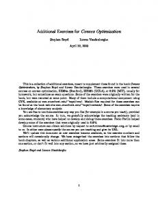
In Fig. 4, we compare the region-filling properties of our method to a standard four-neighborhood approach optimized using alpha-beta-swap. The algorithm converges to a clearly non-binary result; however after binarization we get the correct minimal partition as expected from the continuous formulation. Direct numerical comparison to the graph cut methods is difficult, as the latter rely on binary potentials, while our discretization uses ternary potentials. Fig. 5 demonstrates the applicability of our method for optimization of non-Euclidean distances: The truncated linear distance improves stereo disparity estimation, as it allows for small depth variations within objects and does not excessively penalize depth changes at object borders. To characterize the performance of our optimization method, we compared it to the Arrow-Hurwicz method from [5] with alternating primal and dual proximal steps, applied to our relaxation. The latter method requires to set a step size, which leads to divergence if set too large. We found the upper bound to be dependent on the embedding A. On the Tsukuba data set (Fig. 5), both methods are close, but the convergence speed of the Arrow-Hurwicz method depends on the manually chosen step size (Fig. 6). We also found that our method generally outperforms the theoretical suboptimality bound (22) by a factor of 5 − 10. Since our approach allows to vary the regularization depending on the actual labels, we may introduce classes

3.0 ´ 105

Τ=0.04 Nesterov

2.0 ´ 105 10

20

50

100

200

500

1000

Figure 6. Objective vs. number of iterations N using the ArrowHurwicz method from [5] (dashed) with various choices for the step size τ and our method (solid) on the problem in Fig. 5. The proposed parameter-free Nesterov method shows competitive performance, and outperforms the Arrow-Hurwicz method if the step size is not hand-tuned to the specific dataset.

which differ only by the regularization term. In Fig. 7, the grayscale image was segmented into dark and light background, as well as two foreground classes for text over dark and text over light background with identical data term. By choosing a suitable (originally non-Euclidean) d, this allows to simultaneously separate foreground from background and perform a background reconstruction, which is not possible using the standard Potts distance.

5. Conclusion and Future Work Based on a total variation for vector fields, we showed how to formulate a class of convex spatial regularizers in the continuous multi-labeling framework. The regularizers may depend on arbitrary distances between labels, which are approximated if necessary. Solving the discrete optimization problem using Nesterov’s method showed to be competitive in speed without requiring any parameter tuning. The promising results should motivate to investigate what other kinds of regularizers are possible. The optimization framework allows for many other – possibly higherorder, nonlocal, or spatially varying – regularizers and different relaxations by replacing the constraint sets C and D, with the only requirement that projections on these sets can be computed.

Figure 7. Simultaneous segmentation and background reconstruction by solving a single convex optimization problem within our framework. Left: Noisy image (PSNR = 20.82 dB). Center: Reconstructed background. Right: Extracted foreground. The image was segmented into four classes, and a (non-Euclidean) d was chosen so as to differentiate text over dark and light background.

6. Appendix Proof of Proposition 1. 1. follows from (P2) and (P3) by choosing i = j and S with Per(S) > 0. Symmetry in 2. is obtained from (P3) by replacing S with S c , as Per(S) = Per(S c ). For 3., fix any S with
c := Per(S) > 0, then
cd(i, k) = cJ ei
χS + ek χS c 6 cJ ei χS + ej χS c + J ek χS c + ej χS = c (d (i, j) + d(j, k)) due to (P1). d(i, j) > 0 follows from 1.-3. Proof of Proposition 2. Rearranging the terms and applying Gauss’ theorem to remove the constant part yields Z ⊤ TVv (a + ub) = sup u div (hb, v1 i, . . . , hb, vd i) dx . v∈Dv

Ω

Now for any v ∈ Dv there exists v ′ ∈ Dc s.t. ∀i ∈ For v ∈ Dv , set {1, . . . , d} : hb, vi i = kbkvi′ and vice versa: P vi′ (x) := kbk−1 hb, vi (x)i, then kv ′ (x)k22 6 i kvi (x)k2 6 1. For v ′ ∈ Dc set vi (x) := kbk−1 bvi′ (x), then kv(x)kF = kv ′ (x)k2 6 1. Thus we may substitute hb, vi i = kbkvi′ , and Z TVv (a + ub) = sup ukbk div v ′ dx = kbk TVc (u) . v ′ ∈Dc

Ω

References [1] J.-F. Aujol. Some algorithms for total variation based image restoration. CMLA Preprint, (2008-05), 2008. [2] I. Borg and P. J. F. Groenen. Modern Multidimensional Scaling. Springer, 2nd edition, 2005. [3] Y. Boykov and V. Kolmogorov. An experimental comparison of min-cut/max-flow algorithms for energy minimization in vision. Patt. Anal. Mach. Intell., 26(9):1124–1137, 2004. [4] Y. Boykov, O. Veksler, and R. Zabih. Fast approximate energy minimization via graph cuts. Patt. Anal. Mach. Intell., 23(11):1222–1239, 2001. [5] A. Chambolle, D. Cremers, and T. Pock. A convex approach for computing minimal partitions. Technical Report 649, Ecole Polytechnique CMAP, 2008. [6] T. F. Chan, S. Esedo¯glu, and M. Nikolova. Algorithms for finding global minimizers of image segmentation and denoising models. J. Appl. Math., 66(5):1632–1648, 2006. [7] V. Duval, J.-F. Aujol, and L. Vese. A projected gradient algorithm for color image decomposition. CMLA Preprint, (2008-21), 2008.

[8] J. Gower. Properties of Euclidean and non-Euclidean distance matrices. Lin. Alg. and its Appl., 67:81–97, 1985. [9] H. Ishikawa. Exact optimization for Markov random fields with convex priors. Patt. Anal. Mach. Intell., 25(10):1333– 1336, 2003. [10] C. R. Johnson and P. Tarazaga. Connections between the real positive semidefinite and distance matrix completion problems. Lin. Alg. and its Appl., 223–224:375–391, 1995. [11] J. Kleinberg and E. Tardos. Approximation algorithms for classification problems with pairwise relationships: Metric labeling and Markov random fields. In Found. Comp. Sci., pages 14–23, 1999. [12] V. Kolmogorov and Y. Boykov. What metrics can be approximated by geo-cuts, or global optimization of length/area and flux. Int. Conf. Comp. Vis., 1:564–571, 2005. [13] N. Komodakis and G. Tziritas. Approximate labeling via graph cuts based on linear programming. Patt. Anal. Mach. Intell., 29(8):1436–1453, 2007. [14] J. Lellmann, J. Kappes, J. Yuan, F. Becker, and C. Schn¨orr. Convex multi-class image labeling by simplex-constrained total variation. Tech. rep., Univ. of Heidelberg, 2008. [15] C. Michelot. A finite algorithm for finding the projection of a point onto the canonical simplex of Rn . J. Optim. Theory and Appl., 50(1):195–200, 1986. [16] Y. Nesterov. Smooth minimization of non-smooth functions. Math. Prog., 103(1):127–152, 2004. [17] R. Rockafellar. Convex Analysis. Princeton UP, 1970. [18] G. Sapiro and D. L. Ringach. Anisotropic diffusion of multivalued images with applications to color filtering. In Trans. Image Process., volume 5, pages 1582–1586, 1996. [19] G. Strang. Maximal flow through a domain. Math. Prog., 26:123–143, 1983. [20] R. Szeliski, R. Zabih, D. Scharstein, O. Veksler, V. Kolmogorov, A. Agarwala, M. Tappen, and C. Rother. A comparative study of energy minimization methods for Markov random fields. In Europ. Conf. Comp. Vis., volume 2, pages 19–26, 2006. [21] P. Weiss, G. Aubert, and L. Blanc-F´eraud. Efficient schemes for total variation minimization under constraints in image processing. Tech. Rep. 6260, INRIA, 2007. [22] H. Wolkowicz, R. Saigal, and L. Vandenberghe, editors. Handbook of Semidefinite Programming. Kluwer Academic Publishers, 2000. [23] C. Zach, D. Gallup, J.-M. Frahm, and M. Niethammer. Fast global labeling for real-time stereo using multiple plane sweeps. In Vis. Mod. Vis, 2008.