Real-Time Embedded Convex Optimization

Real-Time Embedded Convex Optimization

Stephen Boyd joint work with Michael Grant, Jacob Mattingley, Yang Wang Electrical Engineering Department, Stanford University

ISMP 2009

Outline

• Real-time embedded convex optimization • Examples • Parser/solvers for convex optimization • Code generation for real-time embedded convex optimization

ISMP 2009

1

Embedded optimization

• embed solvers in real-time applications • i.e., solve an optimization problem at each time step • used now for applications with hour/minute time-scales – process control – supply chain and revenue ‘management’ – trading

ISMP 2009

2

What’s new embedded optimization at millisecond/microsecond time-scales millions problem size −→

traditional problems →

thousands

← our focus tens microseconds

seconds

hours days

solve time −→ ISMP 2009

3

Applications • real-time resource allocation – update allocation as objective, resource availabilities change • signal processing – estimate signal by solving optimization problem over sliding window – replace least-squares estimates with robust (Huber, ℓ1) versions – re-design (adapt) coefficients as signal/system model changes • control – closed-loop control via rolling horizon optimization – real-time trajectory planning • all of these done now, on long (minutes or more) time scales but could be done on millisecond/microsecond time scales ISMP 2009

4

Outline


ISMP 2009

5

Grasp force optimization • choose K grasping forces on object to – resist external wrench (force and torque) – respect friction cone constraints – minimize maximum grasp force • convex problem (second-order cone program or SOCP): maxi kf (i)k2 P (i) (i) ext Q f = f subject to i P (i) (i) (i) ext p × (Q f ) = τ i 1/2 (i) (i)2 (i)2 µifz ≥ fx + fy

minimize

max contact force force equillibrium torque equillibrium friction cone constraints

variables f (i) ∈ R3, i = 1, . . . , K (contact forces) ISMP 2009

6

Example

ISMP 2009

7

Grasp force optimization solve times

• example with K = 5 fingers (grasp points) • reduces to SOCP with 15 vars, 6 eqs, 5 3-dim SOCs • custom code solve time: 50µs (SDPT3: 100ms)

ISMP 2009

8

Robust Kalman filtering • estimate state of a linear dynamical system driven by IID noise • sensor measurements have occasional outliers (failures, jamming, . . . ) • model:

xt+1 = Axt + wt,

yt = Cxt + vt + zt

– wt ∼ N (0, W ), vt ∼ N (0, V ) – zt is sparse; represents outliers, failures, . . . • (steady-state) Kalman filter (for case zt = 0): – time update: x ˆt+1|t = Aˆ xt|t – measurement update: x ˆt|t = x ˆt|t−1 + L(yt − C x ˆt|t−1 ) • we’ll replace measurement update with robust version to handle outliers ISMP 2009

9

Measurement update via optimization • standard KF: x ˆt|t is solution of quadratic problem minimize v T V −1v + (x − x ˆt|t−1)T Σ−1 (x − x ˆt|t−1 ) subject to yt = Cx + v with variables x, v (simple analytic solution) • robust KF: choose x ˆt|t as solution of convex problem minimize v T V −1v + (x − x ˆt|t−1 )T Σ−1 (x − x ˆt|t−1) + λkzk1 subject to yt = Cx + v + z with variables x, v, z (requires solving a QP) ISMP 2009

10

Example

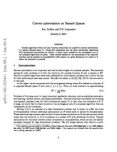
• 50 states, 15 measurements • with prob. 5%, measurement components replaced with (yt)i = (vt)i • so, get a flawed measurement (i.e., zt 6= 0) every other step (or so)

ISMP 2009

11

State estimation error kx − x ˆt|tk2 for KF (red); robust KF (blue); KF with z = 0 (gray)

0.5

ISMP 2009

12

Robust Kalman filter solve time

• robust KF requires solution of QP with 95 vars, 15 eqs, 30 ineqs • automatically generated code solves QP in 120 µs (SDPT3: 120 ms) • standard Kalman filter update requires 10 µs

ISMP 2009

13

Linearizing pre-equalizer • linear dynamical system with input saturation

∗h

y

• we’ll design pre-equalizer to compensate for saturation effects

u

ISMP 2009

equalizer

v

∗h

y

14

Linearizing pre-equalizer

∗h u

e equalizer v

∗h

• goal: minimize error e (say, in mean-square sense) • pre-equalizer has T sample look-ahead capability ISMP 2009

15

• system:

xt+1 = Axt + B sat(vt),

• (linear) reference system:

yt = Cxt

ref xref = Ax t+1 t + But,

ytref = Cxref t

• et = Cxref t − Cxt • state error x ˜t = xref t − xt satisfies x ˜t+1 = A˜ xt + B(ut − vt),

et = C x ˜t

• to choose vt, solve QP Pt+T

2 minimize ˜Tt+T +1P x ˜t+T +1 τ =t eτ + x subject to x ˜τ +1 = A˜ xτ + B(uτ − vτ ), eτ = C x ˜τ , |vτ | ≤ 1, τ = t, . . . , t + T

τ = t, . . . , t + T

P gives final cost; obvious choice is output Grammian ISMP 2009

16

Example

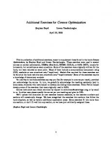
• state dimension n = 3; h decays in around 35 samples • pre-equalizer look-ahead T = 15 samples • input u random, saturates (|ut| > 1) 20% of time

ISMP 2009

17

Outputs desired (black), no compensation (red), equalized (blue) 2.5

0

−2.5

ISMP 2009

18

Errors no compensation (red), with equalization (blue) 0.75

0

−0.75

ISMP 2009

19

Inputs no compensation (red), with equalization (blue) 2.5

0

−2.5

ISMP 2009

20

Linearizing pre-equalizer solve time

• pre-equalizer problem reduces to QP with 96 vars, 63 eqs, 48 ineqs • automatically generated code solves QP in 600µs (SDPT3: 310ms)

ISMP 2009

21

Constrained linear quadratic stochastic control • linear dynamical system:

xt+1 = Axt + But + wt

– xt ∈ Rn is state; ut ∈ U ⊂ Rm is control input – wt is IID zero mean disturbance • ut = φ(xt), where φ : Rn → U is (state feedback) policy • objective: minimize average expected stage cost (Q ≥ 0, R > 0) T −1 1 X T T E xt Qxt + ut Rut J = lim T →∞ T t=0

• constrained LQ stochastic control problem: choose φ to minimize J ISMP 2009

22

Constrained linear quadratic stochastic control • optimal policy has form φ(z) = argmin{v T Rv + E V (Az + Bv + wt)} v∈U

where V is Bellman function – but V is hard to find/describe except when U = Rm (in which case V is quadratic) • many heuristic methods give suboptimal policies, e.g. – projected linear control – control-Lyapunov policy – model predictive control, certainty-equivalent planning ISMP 2009

23

Control-Lyapunov policy • also called approximate dynamic programming, horizon-1 model predictive control • CLF policy is φclf (z) = argmin{v T Rv + E Vclf (Az + Bv + wt)} v∈U

where Vclf : Rn → R is the control-Lyapunov function • evaluating ut = φclf (xt) requires solving an optimization problem at each step • many tractable methods can be used to find a good Vclf • often works really well ISMP 2009

24

Quadratic control-Lyapunov policy • assume – polyhedral constraint set: U = {v | F v ≤ g}, g ∈ Rk – quadratic control-Lyapunov function: Vclf (z) = z T P z • evaluating ut = φclf (xt) reduces to solving QP minimize v T Rv + (Az + Bv)T P (Az + Bv) subject to F v ≤ g

ISMP 2009

25

Control-Lyapunov policy evaluation times • tclf : time to evaluate φclf (z) • tlin: linear policy φlin(z) = Kz • tkf : Kalman filter update • (SDPT3 times around 1000× larger)

ISMP 2009

n

m

k

tclf (µs)

tlin (µs)

tkf (µs)

15

5

10

35

1

1

50

15

30

85

3

9

100

10

20

67

4

40

1000

30

60

298

130

8300

26

Outline


ISMP 2009

27

Parser/solvers for convex optimization • specify convex problem in natural form – declare optimization variables – form convex objective and constraints using a specific set of atoms and calculus rules (disciplined convex programming) • problem is convex-by-construction • easy to parse, automatically transform to standard form, solve, and transform back • implemented using object-oriented methods and/or compiler-compilers • huge gain in productivity (rapid prototyping, teaching, research ideas) ISMP 2009

28

Example: cvx • parser/solver written in Matlab • convex problem, with variable x ∈ Rn; A, b, λ, F , g constants minimize

kAx − bk2 + λkxk1

subject to F x ≤ g • cvx specification: cvx begin variable x(n) % declare vector variable minimize (norm(A*x-b,2) + lambda*norm(x,1)) subject to F*x