Apr 22, 2013 - In this paper, we prove that the superlevel sets of the solutions do not always .... non-monotone on the range [minΩ u,maxΩ u] = [0,maxΩ u] of u (see the .... on âΩ2 by u = 1 (or by any other arbitrary positive real number), ...... in Ω1, whence the limit ζ = limsâ0+ f(·,s)/s is uniform in Ω1 from Dini's theorem.
arXiv:1304.3355v2 [math.AP] 22 Apr 2013
Convexity of level sets for elliptic problems in convex domains or convex rings: two counterexamples Fran¸cois Hamel a,b , Nikolai Nadirashvili a and Yannick Sire a ∗ a Aix-Marseille Universit´e LATP (UMR CNRS 7353), 39 rue F. Joliot-Curie, F-13453 Marseille Cedex 13, France b Institut Universitaire de France
Abstract This paper deals with some geometrical properties of solutions of some semilinear elliptic equations in bounded convex domains or convex rings. Constant boundary conditions are imposed on the single component of the boundary when the domain is convex, or on each of the two components of the boundary when the domain is a convex ring. A function is called quasiconcave if its superlevel sets, defined in a suitable way when the domain is a convex ring, are all convex. In this paper, we prove that the superlevel sets of the solutions do not always inherit the convexity or ring-convexity of the domain. Namely, we give two counterexamples to this quasiconcavity property: the first one for some two-dimensional convex domains and the second one for some convex rings in any dimension.
1
Introduction and main results
This paper is concerned with some geometrical properties of real-valued solutions of semilinear elliptic equations ∆u + f (u) = 0 (1.1) in bounded domains Ω ⊂ RN , in dimensions N = 2 or higher, with Dirichlet-type boundary conditions on ∂Ω. By domains, we mean non-empty open connected subsets of RN . ∗
The research leading to these results has received funding from the French ANR within the project PREFERED and from the European Research Council under the European Union’s Seventh Framework Programme (FP/20072013) / ERC Grant Agreement n.321186 - ReaDi - Reaction-Diffusion Equations, Propagation and Modelling. Part of this work was also carried out during visits by the first author to the Departments of Mathematics of the University of California, Berkeley and of Stanford University, the hospitality of which is thankfully acknowledged.
1
The domains Ω are assumed to be either convex domains or convex rings. One is interested in knowing how these geometrical properties of Ω are inherited by the solutions u, under some suitable boundary conditions, that is how the shape of the solutions is influenced by the shape of the underlying domains. It is well-known that the convexity or the concavity of the solutions are too strong properties which are not true in general (see e.g. [35]). However, a typical question we address in this paper is the following one: assuming that Ω is convex and that u is a solution of (1.1) which is positive in Ω and vanishes on ∂Ω, is it true that the superlevel sets � x ∈ Ω; u(x) > λ of u are all convex? A similar question can be asked when Ω is a convex ring and u is assumed to be equal to two constant values on the two connected components of ∂Ω (see below for detailed statements). These questions have been well studied in the literature: more precisely, almost all papers on this field have been devoted to the proof of a positive answer to these questions, under some suitable conditions on the function f , see the references below. In this paper, we prove that the answer to these questions can also be negative, that is we show that the superlevel sets of some solutions u of problems of the type (1.1) are not all convex. More precisely, we give two counterexamples, one in a class of convex domains and one in a class of convex rings. Let us first deal with the case of bounded convex domains Ω and let us consider the semilinear elliptic problem ∆u + f (u) = 0 in Ω, u = 0 on ∂Ω, (1.2) u > 0 in Ω. Throughout the paper, the function f : [0, +∞) → R is assumed to be locally H¨older continuous. The domains Ω are always assumed to be of class C 2,α (with α > 0, we then say that the domains Ω are �smooth) and the solutions u are understood in the classical sense C 2 (Ω). The superlevel set x ∈ Ω; u(x) > 0 of a solution u of (1.2) is equal to the domain Ω,� which is convex by assumption. A natural question is to know whether the superlevel sets x ∈ Ω; u(x) > λ for λ ≥ 0 are all convex or not. If this is the case, u is called quasiconcave. In his paper [41] (see Remark 3, page 268), P.-L. Lions writes that, in a convex domain Ω, “[he] believe[s] that [...] for general f , the [super]level sets of any solution u of [(1.2)] are convex”. There is indeed a vast literature containing some proofs of the above statement for various nonlinearities f . We here list some of the most classical references. Firstly, Makar-Limanov [42] proved that, for the two-dimensional torsion problem, that is f (u) = 1 with N = 2, the solution u is quasiconcave, √ since u is actually concave. Brascamp and Lieb [14] showed that, if f (u) = λu (λ is then necessarily the principal eigenvalue of the Laplacian with Dirichlet boundary condition), then the principal eigenfunction u is quasiconcave and more precisely it is log-concave, that is log u is concave. The proof uses the fact that log-concavity is preserved by the heat equation (but quasiconcavity is not in general, see [27]). When f (u) = λup with 0 < p < 1 and λ > 0, Keady [32] for N = 2 and Kennington [33] for N ≥ 2 proved that u(1−p)/2 is concave, whence u is quasiconcave. Many generalizations under more general assumptions on f and alternate proofs have been given. A possible strategy is to prove that g(u) is concave for some suitable increasing function g, by 2
showing that g(u(tx + (1 − t)y)) − tg(u(x)) − (1 − t)g(u(y)) ≥ 0 for all (t, x, y) ∈ [0, 1] × Ω × Ω and by using the elliptic maximum principle or the preservation of concavity of g(u) by a suitable parabolic equation, see [17, 25, 30, 31, 33, 34, 35, 41]. Other strategies consist in studying the sign of the curvatures of the level sets of u or in proving that the Hessian matrix of g(u) for some suitable increasing g has a constant rank, see [3, 12, 16, 37, 40, 48]. Lastly, we refer to [5, 23] for further references using the quasiconcave envelope and singular perturbations arguments, and to the book of Kawohl [29] for a general overview. The first main result of this paper is, to our best knowledge, the first counterexample to the quasiconcavity of solutions u of (1.2) in convex domains Ω. Theorem 1.1 In dimension N = 2, there are some smooth bounded convex domains Ω and some C ∞ functions f : [0, +∞) → R such that f (s) ≥ 1 for all s ≥ 0 and for which problem (1.2) admits both a quasiconcave solution v and a solution u which is not quasiconcave. Remark 1.2 When Ω is an Euclidean ball of RN in any dimension N ≥ 1 and when f is locally Lipschitz-continuous, then the celebrated paper of Gidas, Ni and Nirenberg [22] asserts that any solution u of (1.2) is radially symmetric and decreasing with respect to the center of the ball: in other words, the superlevel sets of u are all concentric balls and u is therefore quasiconcave. In particular, Theorem 1.1 cannot hold in dimension N = 1. More generally speaking, if the convex domain Ω is symmetric with respect to some hyperplane, then the moving plane method implies that u itself inherits this property and is actually symmetric and decreasing with respect to the distance to this hyperplane, see [22]. As a matter of fact, the two-dimensional convex domains Ω constructed in the proof of Theorem 1.1 are symmetric with respect to both variables x and y of R2 , whence any solution u of (1.2) is symmetric with respect to x and y, and decreasing with respect to |x| and |y|. These properties imply that the superlevel sets of u are necessarily symmetric and convex with respect to x and y, and starshaped with respect to the origin (0, 0). But the symmetry and convexity properties of the superlevel sets in x and y do not mean that these superlevel sets are truly convex! Actually, they are not so in general, as Theorem 1.1 shows. Remark 1.3 In [15], Cabr´e and Chanillo proved that, if Ω is a smooth bounded strictly convex domain of R2 and if u is any semi-stable solution of (1.2) in the sense that Z Z 2 |∇φ| − f 0 (u)φ2 ≥ 0 Ω
Ω
for every C ∞ (Ω) function φ whose support is compactly included in Ω, then u has a unique critical point (its maximum) and this critical point is nondegenerate, whence the superlevel sets Ωλ of u are convex for λ close to maxΩ u (for further results about the uniqueness and nondegeneracy 3
of the critical point in some more general convex domains Ω, we refer to [6, 15, 44, 47]). If the semi-stability were known to imply the convexity of all superlevel sets (and also in convex domains which are not strictly convex), then the solutions u constructed in Theorem 1.1 would therefore not be semi-stable. However, proving the quasiconcavity from the semi-stability is still an open question, as well as proving or disproving directly the semi-stability of the solutions u of Theorem 1.1. Notice that if f 0 (u) were nonpositive in Ω, then u would be automatically semistable. For the u of Theorem 1.1, the function f 0 (u) is actually equal to 0 on a large set, � solutions and the set x ∈ Ω; f 0 (u(x)) > 0 is always a non-empty open � set (but one can not directly infer the unstability of u from this sole property). Lastly, the set x ∈ Ω; f 0 (u(x)) < 0 is not empty in general for the solutions u of Theorem 1.1, whence f 0 has in general no sign and f is in general non-monotone on the range [minΩ u, maxΩ u] = [0, maxΩ u] of u (see the proof of Theorem 1.1 and Remark 2.5 for more details). In the second part of the paper, we deal with the case of convex rings Ω in any dimension N ≥ 2. Namely, a domain Ω ⊂ RN is called a convex ring if Ω = Ω1 \Ω2 , where Ω1 and Ω2 are two bounded convex domains of RN such that Ω2 ⊂ Ω1 . In a convex ring Ω = Ω1 \Ω2 , let us now consider the semilinear elliptic problem ∆u + f (u) = 0 in Ω, u = 0 on ∂Ω1 , u = M on ∂Ω2 , u > 0 in Ω,
(1.3)
where M > 0 is a positive real number. For any classical solution u of (1.3), we define the function u ∈ C(Ω1 ) by � u(x) if x ∈ Ω, u(x) = M if x ∈ Ω2 = Ω1 \Ω, and we say that u is quasiconcave in Ω if u is so in Ω1 , that is if the superlevel sets � Ωλ := x ∈ Ω1 ; u(x) > λ are convex for all λ� ≥ 0. Notice that Ω 0 = Ω1 is convex by assumption. If we knew that u < M in Ω, T then λ 0, or f (0) = 0 and lim f (s) > λ1 (−∆, Ω1 ) (> 0), s→0+ s where λ1 (−∆, Ω1 ) denotes the smallest eigenvalue of the operator −∆ in Ω1 with Dirichlet boundary condition on ∂Ω1 . Theorem 1.4 Let N be any integer such that N ≥ 2, let Ω1 be any smooth bounded convex domain of RN and let f be any function satisfying (1.4). Then there exists a constant M0 > 0 such that, for all M ≥ M0 , there are some smooth convex rings Ω = Ω1 \Ω2 for which problem (1.3) has a unique solution u and this solution u is not quasiconcave. In Theorem 1.4, the domain Ω1 is any given convex domain and f is any given function satisfying (1.4). One of the main assumptions, quite different from the construction given in [43], is that f 0 (0+ ) is not too small if f (0) = 0. However, even if the function f is assumed to be positive in a right-neighborhood of 0, it may not be nonnegative everywhere. Typical examples of functions f satisfying (1.4) are the positive constants f (s) = β > 0, or functions of the type f (s) = γ s − sp
(1.5)
with p > 1 and γ > λ1 (−∆, Ω1 ) (when γ is a fixed positive constant, this last condition is automatically fulfilled if Ω1 contains a ball with a large enough radius). Notice that for nonlinearities 5
of the type (1.5) with γ > λ1 (−∆, Ω1 ), there exists a unique solution u of problem (1.2) in Ω1 (see [8]) and this solution is log-concave, whence quasiconcave (see [41]). We also point out that Theorem 1.4 holds in any dimension. As a matter of fact, it also holds for equations which are much more general than (1.3), with non-symmetric operators or heterogeneous coefficients. For the sake of clarity of the presentation we prefered to state only the counterexamples for problem (1.3) in the present section. We refer to Section 3 for more general problems. Remark 1.5 In problem (1.3) and in Theorem 1.4, one can replace the boundary condition u = M on ∂Ω2 by u = 1 (or by any other arbitrary positive real number), even if it means changing f . More precisely, if f , Ω1 and M0 > 0 are as in Theorem 1.4, then, for every M ≥ M0 , the function u e = u/M indeed solves ∆e u + fe(e u) = 0 in Ω, u e = 0 on ∂Ω1 , u e = 1 on ∂Ω2 , u e > 0 in Ω, where u and Ω2 as in the statement of Theorem 1.4 and fe(s) = f (M s)/M satisfies the same condition (1.4) as f . Remark 1.6 If, in addition to (1.4), the function f is assumed to be nonpositive for large s, that is there exists a real number µ > 0 such that f (s) ≤ 0 for all s ≥ µ, then one can take M0 = µ in Theorem 1.4 and the solutions u of (1.3) are such that 0 < u < M in Ω for all M ≥ µ. We refer to Remark 3.2 for further details.
2
Counterexamples in convex domains: proof of Theorem 1.1
This section is devoted to the proof of Theorem 1.1. That is, we construct explicit examples of bounded smooth convex two-dimensional domains Ω and of functions f for which problem (1.2) admits some non-quasiconcave solutions u. The construction is divided into five main steps. Firstly, we define a one-parameter family (Ωa )a≥1 of more and more elongated stadium-like convex domains. Secondly, for each value of the parameter a ≥ 1, we solve a variational problem in H01 (Ωa ) with a nonlinear constraint, any solution ua of which solves an elliptic equation of the type (1.2) in Ωa with some function fa . Thirdly, we prove some a priori estimates for the superlevel sets of the functions ua . Next, we compare ua with a one-dimensional profile in Ωa when a is large enough. Lastly, we show that the superlevel sets of the functions ua cannot be all convex when a is large enough. 6
1 �a -a
0
a
-1 Figure 1: The convex stadium-like domain Ωa
As a preliminary step, let us fix a C ∞ function g : R → [0, 1] such that g = 0 on (−∞, 1], g = 1 on [2, +∞) and g 0 ≥ 0 on R.
(2.6)
The function g is fixed throughout the proof. Step 1: construction of a family of smooth bounded convex domains (Ωa )a≥1 . We first introduce a family of stadium-like smooth convex domains. Denote (x, y) the coordinates in R2 . Let ϕ : [−1, 1] → R be a fixed continuous nonnegative concave even function such that ϕ(±1) = 0. For a ≥ 1, we define � Ωa = (x, y) ∈ R2 ; −a − ϕ(y) < x < a + ϕ(y), −1 < y < 1 (2.7) and we choose ϕ once for all so that Ω1 (and then Ωa for every a ≥ 1) be of class C 2,α with α > 0 2,α (this means that ϕ is of class Cloc (−1, 1) and that ϕ satisfies some compatibility conditions at ±1). 2,α The C bounded domains Ωa for a ≥ 1 are all convex and axisymmetric with respect to both axes {x = 0} and {y = 0}, see the joint figure. Our goal is to show that the conclusion of Theorem 1.1 holds with these convex domains Ωa and some functions fa , when a is large enough. Step 2: a constrained variational problem in Ωa . In this step, we fix a parameter a ≥ 1. We construct a C 2,α (Ωa ) function ua as a minimizer of a constrained variational problem in Ωa . Let Ia be the functional defined in H01 (Ωa ) by Z Z 1 2 Ia (u) = |∇u| − u, u ∈ H01 (Ωa ). 2 Ωa Ωa It is well-known that this functional has a unique minimizer in H01 (Ωa ), which is the classi7
cal C 2,α (Ωa ) solution va of the torsion problem ( ∆va + 1 = 0 in Ωa , va = 0 on ∂Ωa .
(2.8)
It follows from the strong maximum principle and the definition of Ωa that 0 < va (x, y)
0 such that ua ≥ m a.e. in Ωa , contradicting the fact that ua ∈ H01 (Ωa ) has a zero trace on R∂Ωa . Hence, g 0 (ua ) cannot be the zero function and the differential of the map H01 (Ωa ) 3 u 7→ Ωa g(u) is not zero at ua . From the Euler-Lagrange formulation and elliptic regularity theory, any such minimizer ua is then a classical C 2,α (Ωa ) solution of an equation of the type ( ∆ua + fa (ua ) = 0 in Ωa , (2.10) ua = 0 on ∂Ωa , where fa (s) = 1 + µa g 0 (s) for s ∈ R and µa ∈ R is a Lagrange multiplier. Observe that the function fa is of class C ∞ (R). Furthermore, ∆(ua − va ) = −µa g 0 (ua )
8
has a constant sign in Ωa , since g 0 is nonnegative. As a consequence of the maximum principle, the function ua − va itself has a constant sign in Ωa . But max ua > 1
(2.11)
Ωa
because of (2.6) and by definition of Ua . Therefore, from (2.9), the function va cannot majorize ua . The strong maximum principle finally implies that 0 < va (x, y) < ua (x, y) for all (x, y) ∈ Ωa .
(2.12)
Thus, the function ua is a classical solution of the problem (1.2) in Ωa with the function fa . Notice also that the sign of ∆(ua − va ) is therefore nonpositive and, since ua and va are not identically equal, one has µa > 0. In particular, fa (s) ≥ 1 for all s ∈ R.
(2.13)
On the other hand, since fa (s) = 1 for all s ≥ 2 because of (2.6), the maximum principle also yields 1 − y2 + 2 for all (x, y) ∈ Ωa . (2.14) ua (x, y) < 2 The uniqueness of the minimizer ua of Ia in the set Ua is not clear, and is anyway not needed in the sequel. However, we point out an important geometrical property fulfilled by ua , which will be used in the next step. Namely, since Ωa is convex and symmetric with respect to the axes {x = 0} and {y = 0}, it follows from [22] that ua is even in x and y and is decreasing with respect to |x| and |y|. In the sequel, we are going to show that, for a large enough, the conclusion of Theorem 1.1 holds with Ωa , fa and ua , that is the minimizers ua have some non-convex superlevel sets. Notice that fa satisfies (2.13), as stated in Theorem 1.1. Before going further on, we also point out that the solution va of the torsion problem (2.8) also solves the same equation (1.2) as ua , with fa in Ωa , because of (2.9) and the fact that fa = 1 on [0, 1] ⊃ [0, 1/2] due to (2.6). Therefore, problem (1.2) with fa in Ωa admits the solution va , which is always quasiconcave by [42] applied to (2.8), whereas the solutions ua will be proved to be non-quasiconcave for a large. Step 3: a priori estimates of the size of a superlevel set of the functions ua . In this step, we study the location of the superlevel sets � ωa = (x, y) ∈ Ωa ; ua (x, y) > 1 of the minimizers ua of Ia in Ua when a is large. From (2.11) and the remarks of the previous step, the sets ωa are non-empty open sets, they are all symmetric with respect to the axes {x = 0} and {y = 0}, and they are convex with respect to both variables x and y. The key-point in this step is to show a uniform control of the size of the sets ωa . We first begin with a bound in the x-direction, meaning that the sets ωa are not too elongated. 9
�a
Cy
ua 1
ua >1
-Cy -Cx
a
Cx
Figure 2: The set ωa where ua > 1
Lemma 2.1 There exists a constant Cx > 0 such that 0 ≤ sup |x| < Cx
(2.15)
(x,y)∈ωa
for all a ≥ 1 and for any minimizer ua of Ia in Ua . Proof. The proof is divided into two main steps. We first estimate from above the quantities Ia (ua ) by introducing a suitable test function in the set Ua , which is not too far from the one-dimensional function y 7→ (1−y 2 )/2. Then, we estimate Ia (ua ) from below by observing that if ua (x, 0) is larger than 1 then the contribution of ua (x, ·) to Ia (ua ) in the section Ωa ∩ ({x} × R) will be uniformly larger than that of the minimizer y 7→ (1 − y 2 )/2. This eventually provides a control of the size of such points x and then of the size of ωa , independently of a. Throughout the proof, one can assume without loss of generality that a is any real number such that a ≥ 2 (since sup(x,y)∈Ωa |x| ≤ a + kϕkL∞ (−1,1) for all a ≥ 1 by the definition (2.7) of Ωa ). We consider any minimizer ua of the functional Ia in the set Ua and we set xa = sup |x|.
(2.16)
(x,y)∈ωa
Let us first bound Ia (ua ) from above by using the minimality of ua and comparing Ia (ua ) with the value of Ia at some suitably chosen test function. Let w be a fixed C ∞ (R2 ) nonnegative function such that w = 0 in R2 \(−1, 1)2 and w > 0 in [−2/3, 2/3]2 . The function w is independent of a. Let φ0 be the H01 (−1, 1) function defined by φ0 (y) =
1 − y2 for all y ∈ [−1, 1]. 2
(2.17)
We point out that φ0 is the unique minimizer in H01 (−1, 1) of the functional J is defined by Z Z 1 1 1 0 2 J(φ) = φ (y) dy − φ(y)dy, φ ∈ H01 (−1, 1). (2.18) 2 −1 −1 10
From Lebesgue’s dominated convergence theorem, the function Z G : t 7→ g(φ0 (y) + t w(x, y)) dx dy (−1,1)2
is continuous in R. Furthermore, G(0) = 0 from (2.6) and (2.17), and Z � 4 �2 lim G(t) = dx dy ≥ > 1. t→+∞ 3 {w(x,y)>0} Therefore, there is t0 ∈ (0, +∞), independent of a, such that Z g(φ0 (y) + t0 w(x, y)) dx dy = 1. G(t0 ) = (−1,1)2
Let us now consider the test function wa defined in Ωa by wa (x, y) = φ0 (y)χa (x) + t0 w(x, y), where χa : R → [0, 1] is even and defined in [0, +∞) by if x ∈ [0, a − 1], 1 a − x if x ∈ (a − 1, a), χa (x) = 0 if x ≥ a. The function wa belongs to H01 (Ωa ). Furthermore, since a ≥ 2, one has wa (x, y) = φ0 (y) + t0 w(x, y) for all (x, y) ∈ (−1, 1)2 , while wa (x, y) = φ0 (y)χa (x) ≤ φ0 (y) < 1 for all (x, y) ∈ Ωa \(−1, 1)2 . Therefore, Z
Z g(wa ) =
Ωa
Z g(wa ) =
(−1,1)2
g(φ0 (y) + t0 w(x, y)) dx dy = G(t0 ) = 1. (−1,1)2
In other words, wa ∈ Ua . By definition of ua , one infers that Ia (ua ) ≤ Ia (wa ).
(2.19)
Let us now estimate Ia (wa ) from above. By using the facts that the domain Ωa is symmetric in x and that the function χa is even in x and by decomposing the integral Ia (wa ) into three subdomains, one gets that Z Z |∇(φ0 (y) + t0 w(x, y))|2 dx dy − (φ0 (y) + t0 w(x, y)) dx dy Ia (wa ) = 2 (−1,1)2 (−1,1)2 Z Z |∇φ0 (y)|2 +2 dx dy − 2 φ0 (y) dx dy 2 (2.20) (1,a−1)×(−1,1) (1,a−1)×(−1,1) Z Z 2 |∇(φ0 (y)χa (x))| +2 dx dy − 2 φ0 (y)χa (x) dx dy 2 (a−1,a)×(−1,1) (a−1,a)×(−1,1) = 2(a − 2)J(φ0 ) + β, 11
where β is a real number which does not depend on a (it is indeed immediate to see by setting x = x0 + a in the last two integrals of (2.20) that these quantities do not depend on a). Finally, it follows from (2.19) and (2.20) that Ia (ua ) ≤ 2(a − 2)J(φ0 ) + β.
(2.21)
In the second step, we bound Ia (ua ) from below. On the set Ωa \(−a, a) × (−1, 1), one simply uses the fact that Z Z � |∇u |2 � 5 a − ua ≥ − ≥ −10kϕkL∞ (−1,1) 2 Ωa \(−a,a)×(−1,1) Ωa \(−a,a)×(−1,1) 2 from (2.14) and from the definition (2.7) of Ωa . Therefore, Z � � |∇u |2 a − ua − 10kϕkL∞ (−1,1) Ia (ua ) ≥ 2 Z(−a,a)×(−1,1) a ≥ J(ua (x, ·)) dx − 10kϕkL∞ (−1,1) ,
(2.22)
−a
where the functional J has been defined in (2.18) and where we have used the fact that ua (x, ·) belongs to H01 (−1, 1) for all x ∈ (−a, a). Remember that φ0 is the (unique) minimizer of J. As a consequence, J(ua (x, ·)) ≥ J(φ0 ) for all x ∈ (−a, a). (2.23) On the other hand, by definition of xa in (2.16) and by convexity and symmetry of ωa with respect to both variables x and y, it follows that (x, 0) ∈ ωa for all x ∈ (−xa , xa ), whence ua (x, 0) > 1 > φ0 (0) for all x ∈ (−xa , xa ). Hence, there is a positive real number γ > 0, independent of a, such that kua (x, ·) − φ0 kH 1 (−1,1) ≥ γ > 0 for all x ∈ (−xa , xa ). By definition of φ0 and from the coercivity of the functional J, one infers the existence of a positive constant δ > 0, independent of a, such that J(ua (x, ·)) ≥ J(φ0 ) + δ for all x ∈ (−xa , xa ). From (2.22) and (2.23), one then gets that Ia (ua ) ≥ 2δ min(xa , a) + 2aJ(φ0 ) − 10kϕkL∞ (−1,1) .
(2.24)
Putting together (2.21) and (2.24) with the inequality xa − kϕkL∞ (−1,1) ≤ min(xa , a) yields 2δ(xa − kϕkL∞ (−1,1) ) + 2aJ(φ0 ) − 10kϕkL∞ (−1,1) ≤ 2(a − 2)J(φ0 ) + β, where β > 0 and δ > 0 are independent of a. Hence, there exists a constant Cx > 0, independent of a, such that 0 ≤ xa < Cx , that is (2.15). The proof of Lemma 2.1 is thereby complete. � The second lemma gives a bound from below of the “vertical” size of the sets ωa , meaning that the sets ωa are not too thin. 12
Lemma 2.2 There exists a constant Cy > 0 such that 0 < Cy < sup |y|
(2.25)
(x,y)∈ωa
for all a ≥ 1 and for any minimizer ua of Ia in Ua . Proof. It is actually an immediate consequence of Lemma 2.1 and of the constraint in the definition of the sets Ua . Consider any real number a ≥ 1 and any minimizer ua of the functional Ia in the set Ua . Denote (2.26) ya = sup |y|. (x,y)∈ωa
There holds ya > 0 since ωa is open and non-empty. Nevertheless, we want to get a lower bound that is independent of a. By Lemma 2.1 and by definition of xa and ya in (2.16) and (2.26), there holds ua ≤ 1 in Ωa \ (−Cx , Cx ) × (−ya , ya ), whence g(ua ) = 0 in this set, using (2.6). Therefore, since ua ∈ Ua and g ≤ 1 in R, it follows that Z Z 1= g(ua ) = g(ua ) ≤ 4 Cx ya . Ωa
Ωa ∩ (−Cx ,Cx )×(−ya ,ya )
In other words, the conclusion (2.25) holds with Cy such that 0 < Cy < (4Cx )−1 .
�
Step 4: comparison of ua (x, y) with φ0 (y) when a is large. In this step, we prove that the minimizers ua of Ia in Ua are close to the one-dimensional profile φ0 (y) = (1 − y 2 )/2 far away from the origin and far away from the leftmost and rightmost points of Ωa in the direction x. Lemma 2.3 For all ε > 0, there exist A ≥ 1 and M ∈ [0, A/2] such that � 1 − y 2 |ua (x, y) − φ0 (y)| = ua (x, y) − ≤ ε in [−a + M, −M ] ∪ [M, a − M ] × [−1, 1] (⊂ Ωa ), 2 for all a ≥ A and for any minimizer ua of Ia in Ua . Proof. Assume that the conclusion does not hold for some ε > 0. Then there are some sequences (an )n∈N and (xn , yn )n∈N of real numbers and points in R2 such that an ≥ n,
n n ≤ |xn | ≤ an − , |yn | ≤ 1, |uan (xn , yn ) − φ0 (yn )| > ε for all n ∈ N, 2 2
(2.27)
where uan is a minimizer of the functional Ian in the set Uan . For each n ∈ N, define � un (x, y) = uan (x + xn , y) for all (x, y) ∈ Ωan − (xn , 0) = (x, y) ∈ R2 ; (x + xn , y) ∈ Ωan . Each function un satisfies a semilinear elliptic equation of the type (2.10) in Ωan − (xn , 0) with a nonlinearity fan = 1 + µan g 0 for some µan ∈ R. Lemma 2.1 and (2.12) imply that 0 < uan (x, y) ≤ 1 for all n ∈ N and (x, y) ∈ Ωan \(−Cx , Cx ) × (−1, 1). 13
Hence, because of (2.6) and (2.27), for every fixed C ≥ 0, there holds 0 ≤ un (x, y) ≤ 1 and ∆un (x, y) + 1 = 0 for all (x, y) ∈ [−C, C] × [−1, 1], for all n large enough. From standard elliptic estimates up to the boundary, it follows that, up to 2 (R×[−1, 1]) to a classical solution u∞ extraction of a subsequence, the functions un converge in Cloc of ∆u∞ + 1 = 0 in R × [−1, 1], 0 ≤ u∞ ≤ 1 in R × [−1, 1], u∞ = 0 on R × {±1}. Withtout loss of generality, one can also assume that yn → y∞ ∈ [−1, 1] as n → +∞, whence |u∞ (0, y∞ ) − φ0 (y∞ )| ≥ ε
(2.28)
from (2.27). On the other hand, a standard Liouville-type result implies that u∞ is necessarily identically equal to the one-dimensional profile φ0 (y) in R × [−1, 1]. Indeed, the function h(x, y) = u∞ (x, y) − φ0 (y) is bounded and harmonic in R × [−1, 1], and it vanishes on R × {±1}. The maximum principle implies that � πx � � πy � cosh |h(x, y)| ≤ η cos 4 4 for all (x, y) ∈ R × [−1, 1] and for all η > 0 (otherwise, the inequality would hold in R × [−1, 1] for some η ∗ > 0, with equality at some point in R × (−1, 1), contradicting the strong maximum principle). Thus, since η > 0 can be arbitrarily small, one gets that h(x, y) = 0 for all (x, y) ∈ R×[−1, 1]. In other words, u∞ (x, y) = φ0 (y) for all (x, y) ∈ R × [−1, 1]. This is in contradiction with (2.28) and the proof of Lemma 2.3 is thereby complete.
�
Step 5: the superlevel sets of the minimizers ua cannot be all convex when a is large enough. In this last step, we complete the proof of Theorem 1.1. Actually, Lemma 2.2 and the one-dimensional convergence given in Lemma 2.3 will prevent any minimizer ua of Ia in Ua from being quasiconcave when a is large enough. Given Cy > 0 as in Lemma 2.2, let P , Qa and Ra be the points of R2 whose coordinates are given by �a C � �a � y P = (0, Cy ), Qa = , and Ra = ,0 4 2 2 for all a ≥ 1, see the joint figure. From Lemma 2.2 and the convexity and symmetry of ωa with respect to x and y, there holds P ∈ ωa , that is ua (P ) > 1 for any minimizer ua of Ia in Ua . On the other hand, the point Ra belongs to Ωa for all a ≥ 1 by definition (2.7) of Ωa and the point Qa is at the middle of the segment [P, Ra ] and is thus in Ωa too by convexity of Ωa . 14
�a
P
Qa
Ra
a/4
a/2
Figure 3: The aligned points P , Qa and Ra
Furthermore, Lemma 2.3 implies that ua (Qa ) −→
1 Cy2 1 1 − (Cy /2)2 = − and ua (Ra ) −→ as a → +∞, 2 2 8 2
for any minimizer ua of Ia in Ua . As a consequence, given any real number λ such that 1 1 Cy2 − λ (2.29) of any minimizer ua of Ia in Ua is not convex, whence ua is not quasiconcave. The proof of Theorem 1.1 is thereby complete. � ea = (εa, (1 − 2ε)Cy ) and by choosing ε ∈ (0, 1/2) arbitrarily Remark 2.4 By replacing Qa by Q small, it follows from the above arguments that, given any real number λ such that 1 − Cy2 1 0 is never empty. Indeed, if Ea+ were empty, then g 00 = fa0 /µa would be nonpositive on the range of ua , that is on the interval [0, maxΩa ua ]. Due to (2.6), that would mean that g is actually constant equal to 0 on this interval [0, maxΩa ua ], whence fa (ua ) = 1 + µa g 0 (ua ) = 1 in Ωa . That would imply that ua = va in Ωa , which is not the case. Thus, the open set Ea+ cannot be the empty set. On the other hand, the set � Ea− = (x, y) ∈ Ωa ; fa0 (ua (x, y)) < 0 is not empty in general. Indeed, let for instance θ be the function defined in (1, 2) by � � 1 1 θ(s) = e− s−1 − 2−s sin
� � 1 + 1 , s ∈ (1, 2) (s − 1)2
and let the function g be defined by 0 if s ≤ 1, Z s θ(t) dt if 1 < s < 2, κ g(s) = 1 1 if s ≥ 2, where the constant κ > 0 is chosen so that g is continuous at s = 2. The function g is then of class C ∞ (R) and it satisfies (2.6). But g 00 has infinitely many sign changes in any right neighborhood of 1. For this choice of g and for any minimizer ua of Ia in Ua with a ≥ 1, since 0 = minΩa ua < 1 < maxΩa ua and fa0 (ua ) = µa g 00 (ua ), it follows that the set Ea− is not empty.
3
Counterexamples in convex rings
In this section, we consider problems of the type (1.3) set in convex rings Ω = Ω1 \Ω2 . The examples of non-convexity of some superlevel sets of the solutions of (1.3) stated in Theorem 1.4 can be viewed as a particular case of a more general statement. Namely, we shall construct counterexamples for the convexity of the superlevel sets of the solutions of heterogeneous nonsymmetric semilinear elliptic equations of the type ∇ · (A(x)∇u) + b(x) · ∇u + f (x, u) = 0 in Ω, u = 0 on ∂Ω1 , (3.30) u = M on ∂Ω2 , u > 0 in Ω, 16
where M > 0 is a positive real number and Ω = Ω1 \Ω2 is a convex ring. The convex domain Ω1 is given and its boundary is smooth, in the sense that it is of class C 2,α with α > 0. The convex interior domain Ω2 such that Ω2 ⊂ Ω1 shall be constructed later, in the proof of Theorem 3.1 below. The coefficients A and b are given in Ω1 and f in Ω1 × [0, +∞). More precisely, the matrix field A : x 7→ A(x) = (aij (x))1≤i,j≤N is a symmetric matrix field of class C 1,α (Ω1 ) such that X ∃ β > 0, ∀ x ∈ Ω1 , ∀ ξ = (ξi )1≤i≤N ∈ RN , aij (x) ξi ξj ≥ β |ξ|2 , 1≤i,j≤N 2 where |ξ|2 = ξ12 + · · · + ξN . The vector field b : x 7→ b(x) = (bi (x))1≤i≤N is of class C 0,α (Ω1 ) and the function f : Ω1 × [0, +∞), (x, s) 7→ f (x, s) is of class C 0,α (Ω1 ) with respect to x locally in s and locally Lipschitz-continuous with respect to s uniformly in x. Furthermore, we assume that f is bounded from above, that is sup f (x, s) < +∞, (x,s)∈Ω ×[0,+∞) 1 s 7→ f (x, s) is nonincreasing over (0, +∞) for all x ∈ Ω1 , s (3.31) f (e x, s) is decreasing over (0, +∞) for some x e ∈ Ω1 , s 7→ s either max f (·, 0) > 0, or f (·, 0) = 0 in Ω1 and λ1 (−L, Ω1 ) < 0, Ω1
where
L = ∇ · (A(x)∇) + b(x) · ∇ + ζ(x), f (x, s) ζ(x) = lim s→0+ s and λ1 (−L, Ω1 ) denotes the principal eigenvalue of the operator −L in Ω1 with Dirichlet boundary condition on ∂Ω1 . In the case f (·, 0) = 0 in Ω1 , we assume moreover that ζ is H¨older-continuous in Ω1 , whence the limit ζ = lims→0+ f (·, s)/s is uniform in Ω1 from Dini’s theorem. In this case, the principal eigenvalue λ1 (−L, Ω1 ) of the operator −L with Dirichlet boundary condition on ∂Ω1 is a real number which is characterized by the existence and uniqueness (up to multiplication) of a classical eigenfunction ϕ solving −Lϕ = λ1 (−L, Ω1 ) ϕ in Ω1 , (3.32) ϕ = 0 on ∂Ω1 , ϕ > 0 in Ω1 , see [11].1 Theorem 1.4 can then be viewed as a particular case of the following result. 1
When maxΩ1 f (·, 0) > 0, if we define Ls = ∇·(A(x)∇)+b(x)·∇+f (x, s)/s for all s > 0, the map s 7→ λ1 (−Ls , Ω1 ) is nondecreasing on (0, +∞) and one can then set λ1 (−L, Ω1 ) = lims→0+ λ1 (−Ls , Ω1 ). On the other hand, f (·, s)/s → +∞ as s → 0+ at least uniformly in a subdomain of Ω1 . Since λ1 (−Ls , ·) is nonincreasing with respect to the inclusion of domains for each s > 0 (see [11]), it follows that λ1 (−L, Ω1 ), as defined as above, is equal to −∞.
17
Theorem 3.1 Let N be any integer such that N ≥ 2, let Ω1 be any smooth bounded convex domain of RN , let A and b be as above and let f be any function satisfying (3.31) with ζ being H¨ oldercontinuous in Ω1 in case f (·, 0) = 0 in Ω1 . Then there exists a constant M0 > 0 such that, for all M ≥ M0 , there are some smooth convex rings Ω = Ω1 \Ω2 for which problem (3.30) has a unique solution u and this solution u is not quasiconcave. Proof. Let N , Ω1 , A, b and f be as in the statement. The strategy of the proof consists in the following steps: we first construct and prove the uniqueness of a solution v of the boundary value problem ∇ · (A(x)∇v) + b(x) · ∇v + f (x, v) = 0 in Ω1 , v = 0 on ∂Ω1 , (3.33) v > 0 in Ω1 ; next, for M0 = maxΩ1 v, for any point x0 ∈ Ω1 such that v(x0 ) < maxΩ1 v and for Ω2 being a smooth convex domain included in the Euclidean ball B(x0 , ε) of center x0 and radius ε > 0 small enough, we prove the existence and uniqueness of a solution u of (3.30) with Ω = Ω1 \Ω2 and M ≥ M0 ; by uniqueness of v, this solution u shall be close to v locally in Ω1 \{x0 } for ε > 0 small enough, from standard elliptic estimates and a priori bounds; the conclusion, that is u has some non-convex superlevel sets for ε > 0 small enough, will then follow from the choice of x0 and the fact that M ≥ maxΩ1 v. Step 1: problem (3.33) in Ω1 . Let us first prove the existence and uniqueness of a solution v of (3.33) in Ω1 . The proof draws its inspiration from [8, 9, 10], where f is usually assumed to be nonpositive for s large enough (instead of being globally bounded from above). We adapt the method with the weaker assumptions (3.31). Let ψ be the unique C 2,α (Ω1 ) solution of the boundary value problem ( ∇ · (A(x)∇ψ) + b(x) · ∇ψ = −1 in Ω1 , (3.34) ψ = 0 on ∂Ω1 . The function ψ is such that ψ > 0 in Ω1 from the strong maximum principle. Let C be a positive real number such that (3.35) f (x, s) ≤ C for all (x, s) ∈ Ω1 × [0, +∞). It follows that the function Cψ is a supersolution of the equation (3.33) in Ω1 , in the sense that ∇ · (A(x)∇(Cψ)) + b(x) · ∇(Cψ) + f (x, Cψ) ≤ ∇ · (A(x)∇(Cψ)) + b(x) · ∇(Cψ) + C = 0 in Ω1 . Furthermore, Hopf’s lemma implies that ∂ψ/∂ν < 0 on ∂Ω1 , where ν denotes the outward unit normal on ∂Ω1 . In order to construct a subsolution of (3.33), we first consider the case when f (·, 0) = 0 in Ω1 and λ1 (−L, Ω1 ) < 0. Let ϕ be a classical solution of the eigenvalue problem (3.32) in Ω1 . Since
18
the convergence f (·, s)/s → ζ as s → 0+ is uniform in Ω1 and since λ1 (−L, Ω1 ) < 0, it follows that there exists δ0 > 0 such that, for all δ ∈ (0, δ0 ), ∇ · (A(x)∇(δϕ)) + b(x) · ∇(δϕ) + f (x, δϕ) ≥ 0 in Ω1 , δϕ = 0 on ∂Ω1 , (3.36) δϕ > 0 in Ω1 . In other words, δϕ is a subsolution of problem (3.33) in Ω1 for δ > 0 small enough. Furthermore, since ψ > 0 in Ω1 , ∂ψ/∂ν < 0 on ∂Ω1 , ψ and ϕ both vanish on ∂Ω1 and ϕ is (at least) of class C 1 (Ω1 ), there holds δϕ ≤ Cψ in Ω1 for δ > 0 small enough. For some given small enough δ > 0, the monotone iteration method yields the existence of a solution v of (3.33) such that δϕ ≤ v ≤ Cψ in Ω1 . Consider now the case when maxΩ1 f (·, 0) > 0. Let B be a non-empty open Euclidean ball such that B ⊂ Ω1 and minB f (·, 0) > 0. Let φ be any C 2 (B) function such that φ > 0 in B and φ = 0 on ∂B. There exists then δe0 > 0 such that, for all δ ∈ (0, δe0 ), ∇ · (A(x)∇(δφ)) + b(x) · ∇(δφ) + f (x, δφ) ≥ 0 in B, δφ = 0 on ∂B, (3.37) δφ > 0 in B. On the other hand, there holds f (x, 0) ≥ 0 for all x ∈ Ω1
(3.38)
because f (x, s)/s is nonincreasing in s ∈ (0, +∞) for all x ∈ Ω1 . Hence, the function δφ extended by 0 in Ω1 \B is a subsolution of problem (3.33) in Ω1 , for δ > 0 small enough. Furthermore, δφ ≤ Cψ in B for δ > 0 small enough. As above, one then gets the existence of a solution v of (3.33) such that ( v ≤ Cψ in Ω1 , v ≥ δφ in B and v ≥ 0 in Ω1 \B for some given small enough δ > 0. Notice in particular that v > 0 in Ω1 from (3.38) and the strong maximum principle. Lastly, let us prove the uniqueness of the solution v of (3.33). Let w be another solution of (3.33). Since v and w are at least of class C 2 (Ω1 ) and the constant 0 is always a subsolution of problem (3.33) (because f (·, 0) ≥ 0 in Ω1 ), Hopf’s lemma implies that ∂v/∂ν < 0 and ∂w/∂ν < 0 on ∂Ω1 . It follows that there exists a constant τ ≥ 1 such that τ −1 w ≤ v ≤ τ w in Ω1 . 19
Let t∗ ∈ [τ −1 , τ ] be defined as � t∗ = min t > 0, v ≤ t w in Ω1 . Assume that t∗ > 1. Since f (x, s)/s is nonincreasing with respect to s ∈ (0, +∞) for all x ∈ Ω1 and decreasing for at least a point x e in Ω1 , it follows that ∇ · (A(x)∇(t∗ w)) + b(x) · ∇(t∗ w) + f (x, t∗ w) � ≤, 6≡ t∗ ∇ · (A(x)∇w) + b(x) · ∇w + f (x, w) = 0
(3.39)
in Ω1 , while v ≤ t∗ w in Ω1 . One infers from the strong maximum principle that either v < t∗ w in Ω1 or v = t∗ w in Ω1 . The first case is impossible since it would then imply that v ≤ (t∗ − ε)w in Ω1 for all ε > 0 small enough, using again Hopf’s lemma, and it would contradict the definition of t∗ . Thus, v = t∗ w in Ω1 , which is also impossible since the inequality (3.39) is not an equality everywhere. As a consequence, t∗ ≤ 1, whence v ≤ w in Ω1 . Reversing the roles of v and w leads to the conclusion v = w in Ω1 . Step 2: Problem (3.30) in suitable convex rings Ω = Ω1 \Ω2 . Set M0 = maxΩ1 v > 0 and pick any constant M such that M ≥ M0 = max v. (3.40) Ω1
Let us prove the existence of convex smooth domains Ω2 such that Ω2 ⊂ Ω1 and for which problem (3.30) has a unique solution u in Ω = Ω1 \Ω2 and this solution has some non-convex superlevel sets. To do so, pick any point x0 ∈ Ω1 such that v(x0 ) < max v,
(3.41)
Ω1
let ω2 be any (smooth, that is of class C 2,α ) convex domain of RN and consider convex rings of the type Ωε = Ω1 \Ωε2 , with Ωε2 = x0 + ε ω2 for ε > 0 small enough: namely, there is ε∗ > 0 such that Ωε2 ⊂ Ω1 and Ωε is then a convex ring for all ε ∈ (0, ε∗ ). Without loss of generality, one can also assume that there is a fixed real number r > 0 such that Ωε2 ⊂ B(x0 , r) ⊂ Ω1 for all ε ∈ (0, ε∗ ), where B(x0 , r) denotes the open Euclidean ball of center x0 and radius r > 0. Remember that ψ is defined by (3.34) in Ω1 . Since ψ is continuous and positive in Ω1 , there holds Dψ → +∞ locally uniformly in Ω1 as D → +∞ (in particular, minB(x0 ,r) Dψ → +∞ as D → +∞). On the other hand, for all D ≥ C, one has ∇ · (A(x)∇(Dψ)) + b(x) · ∇(Dψ) + f (x, Dψ) ≤ −D + C ≤ 0 in Ω1 20
because of (3.34) and (3.35). Therefore, there is a positive constant D ≥ C such that the function Dψ is a supersolution of problem (3.30) in the convex ring Ωε for all ε ∈ (0, ε∗ ) (in particular, one has Dψ ≥ M on ∂Ωε2 ). On the other hand, when f (·, 0) = 0 in Ω1 , let ϕ solve the eigenvalue problem (3.32) in Ω1 and let δ > 0 be small enough so that δkϕkL∞ (Ω1 ) < M, δϕ ≤ Dψ in Ω1 and δϕ be a subsolution of (3.33) in Ω1 , that is δϕ satisfies (3.36). Choosing such a δ > 0 is possible since ψ > 0 in Ω1 , ∂ψ/∂ν < 0 on ∂Ω1 and ϕ is (at least) of class C 1 (Ω1 ). The function δϕ is then a subsolution of problem (3.30) in Ωε for all ε ∈ (0, ε∗ ). When maxΩ1 f (·, 0) > 0, let B and φ be as in Step 1 and let δ > 0 small enough so that δkφkL∞ (B) < M, δφ ≤ Dψ in B and δφ (extended by 0 in Ω1 \B) be a subsolution of (3.33) in Ω1 , that is δφ satisfies (3.37). The function δφ (extended by 0 in Ω1 \B) is then a subsolution of problem (3.30) in Ωε for all ε ∈ (0, ε∗ ). In both cases f (·, 0) = 0 in Ω1 and maxΩ1 f (·, 0) > 0, for every ε ∈ (0, ε∗ ), there exists a solution uε of (3.30) in Ωε such that f (·, 0) = 0 in Ω1 =⇒ δϕ ≤ uε ≤ Dψ in Ωε , (3.42) ε ε max f (·, 0) > 0 =⇒ δφ ≤ u ≤ Dψ in Ωε ∩ B and 0 ≤ u ≤ Dψ in Ωε \B. Ω1
In particular, since uε is nonnegative by construction and not identically equal to 0 in Ωε (because, for instance, uε = M > 0 on ∂Ωε2 ) and since 0 is always a subsolution of problem (3.30) (because f (·, 0) ≥ 0 in Ω1 ), the strong maximum principle yields uε > 0 in Ωε . Observe now that, if v ε is another solution of (3.30) in Ωε , then the equality uε = t v ε in Ωε for some t > 0 with t 6= 1 is impossible due to the boundary condition on ∂Ωε2 . Therefore, by using the same method as in Step 1, whether x e be in Ωε2 or not, it follows that the solution uε of (3.30) in Ωε is unique. Step 3: non-convexity of some superlevel sets of uε in Ωε for ε > 0 small enough. We now complete the proof of Theorem 3.1. We first claim that 2 uε → v in Cloc (Ω1 \{x0 }) as ε → 0+ ,
(3.43)
where v denotes the unique solution of (3.33), given in Step 1. To prove this claim, let (εn )n∈N be any sequence of real numbers in (0, ε∗ ) such that εn → 0+ as n → +∞. The sequence (kuεn kL∞ (Ωεn ) )n∈N is bounded from (3.42) (remember that the constant D is independent of ε). For any compact subset K ⊂ Ω1 \{x0 }, the sequence (uεn )n≥n0 is then bounded in C 2,α (K) for n0 large enough, from standard elliptic estimates and from the definition 2 of Ωε . Up to extraction of a subsequence, the functions uεn converge as n → +∞ in Cloc (Ω1 \{x0 }) to a C 2 (Ω1 \{x0 }) solution u0 of ( ∇ · (A(x)∇u0 ) + b(x) · ∇u0 + f (x, u0 ) = 0 in Ω1 \{x0 }, u0 = 0 on ∂Ω1 21
such that 0 ≤ δϕ ≤ u0 ≤ Dψ in Ω1 \{x0 } when f (·, 0) = 0 in Ω1 , resp. 0 ≤ δφ ≤ u0 ≤ Dψ in B\{x0 } and 0 ≤ u0 ≤ Dψ in (Ω1 \B)\{x0 } when maxΩ1 f (·, 0) > 0 (remember that the positive constants δ and D are independent of ε). Since the set {x0 } is removable [7, 46], it follows that u0 can be extended to a C 2 (Ω1 ) solution of (3.33). In particular, notice that the positivity of u0 in Ω1 follows from the strong maximum principle and the lower bound u0 ≥ δϕ in Ω1 when f (·, 0) = 0 in Ω1 , resp. u0 ≥ δφ in B when maxΩ1 f (·, 0) > 0. From Step 1 and the uniqueness of the solution of (3.33), one gets that u0 = v in Ω1 , 2 whence uεn → v in Cloc (Ω1 \{x0 }) as n → +∞. Since the limit does not depend on the sequence (εn )n∈N , the claim (3.43) follows. To get the conclusion of Theorem 3.1, it is then sufficient to prove that the solutions uε of (3.30) in Ωε have some non-convex superlevel sets, at least for ε > 0 small enough. Assume by contradiction that this conclusion does not hold, that is there is a sequence (εn )n∈N in (0, ε∗ ) such that εn → 0+ as n → +∞ and, for each n ∈ N, the superlevel sets of the function uεn are all convex. For each n ∈ N, extend the function uεn by M in Ωε2n = x0 + εn ω2 , and still call uεn this extension, now defined in Ω1 . Fix a point y ∈ Ω1 such that
v(y) = max v > 0
(3.44)
Ω1
and let (xn )n∈N be any sequence of points in Ω1 such that xn ∈ Ωε2n for all n ∈ N. Lastly, let η > 0 be an arbitrary positive real number. Since y 6= x0 from (3.41) and (3.44), the convergence (3.43) implies in particular that uεn (y) → v(y) as n → +∞. Therefore, there is n0 ∈ N such that uεn (y) ≥ v(y) − η for all n ≥ n0 . On the other hand, uεn (xn ) = M ≥ M0 = maxΩ1 v = v(y) from (3.40) and (3.44). Since the superlevel sets of uεn in Ω1 are assumed to be all convex, it follows that uεn (x) ≥ v(y) − η for all x ∈ [xn , y] and for all n ≥ n0 , where [xn , y] denotes the segment between xn and y, that is [xn , y] = {txn + (1 − t)y, 0 ≤ t ≤ 1}. From (3.43) and the fact that xn → x0 as n → +∞, one infers that v(x) ≥ v(y)−η for all x ∈ (x0 , y], and then also at the point x = x0 be continuity of v. Since η > 0 is arbitrary, it follows that v(x0 ) ≥ v(y) = max v, Ω1
which is ruled out due to the choice of x0 in (3.41). One has then reached a contradiction and the proof of Theorem 3.1 is thereby complete. � 22
Remark 3.2 When, in addition to (3.31), the function f is nonpositive for large s uniformly in x, that is there exists a constant µ > 0 such that f (x, s) ≤ 0 for all (x, s) ∈ Ω1 × [µ, +∞), then any constant M such that M ≥ µ is a supersolution of problem (3.33) in Ω1 and (3.30) in Ωε (for ε > 0 small enough). Therefore, from the strong maximum principle, for any constant M ≥ µ, the unique solution v of (3.33) in Ω1 and the unique solution uε of (3.30) in Ωε satisfy v < M in Ω1 and uε < M in Ωε for ε > 0 small enough.
References [1] A. Acker, On the nonconvexity of solutions in free-boundary problems arising in plasma physics and fluid dynamics, Comm. Pure Appl. Math. 42 (1989), 1165-1174. Addendum, Comm. Pure Appl. Math. 44 (1991), 869-872. [2] A. Acker, On the uniqueness, monotonicity, starlikeness, and convexity of solutions for a nonlinear boundary value problem in elliptic PDEs, Nonlinear Anal. Theo. Meth. Appl. 22 (1994), 697-705. [3] A. Acker, L.E. Payne, G. Philippin, On the convexity of level lines of the fundamental mode in the clamped membrane problem, and the existence of convex solutions in a related free boundary problem, Z. Angew. Math. Phys. 32 (1981), 683-694. [4] A. Acker, M. Poghosyan, H. Shahgholian, Convex configurations for solutions to semilinear elliptic problems in convex rings, Comm. Part. Diff. Equations 31 (2006), 1273-1287. [5] O. Alvarez, J.-M. Lasry, P.-L. Lions, Convex viscosity solutions and state constraints, J. Math. Pures Appl. 76 (1997), 265-288. [6] J. Arango, A. G´ omez, Critical points of solutions to quasilinear elliptic problems, Nonlinear Anal. 75 (2012), 4375-4381. [7] D.G. Aronson, Removable singularities for linear parabolic equations, Arch. Ration. Mech. Anal. 17 (1964), 79-84. [8] H. Berestycki, Le nombre de solutions de certains probl`emes semi-lin´eaires elliptiques, J. Funct. Anal. 40 (1981), 1-29. [9] H. Berestycki, F. Hamel, L. Roques, Analysis of the periodically fragmented environment model. I - Species persistence, J. Math. Biol. 51 (2005), 75-113. [10] H. Berestycki, F. Hamel, L. Rossi, Liouville type results for semilinear elliptic equations in unbounded domains, Ann. Mat. Pura Appl. 186 (2007), 469-507. [11] H. Berestycki, L. Nirenberg, S.R.S. Varadhan, The principal eigenvalue and maximum principle for second order elliptic operators in general domains, Comm. Pure Appl. Math. 47 (1994), 47-92. [12] B. Bian, P. Guan, X.-N. Ma, L. Xu, A constant rank theorem for quasiconcave solutions of fully nonlinear partial differential equations, Indiana Univ. Math. J. 60 (2011), 101-119. [13] C. Bianchini, M. Longinetti, P. Salani, Quasiconcave solutions to elliptic problems in convex rings, Indiana Univ. Math. J. 58 (2009), 1565-1589.
23
[14] H.J. Brascamp, E.H. Lieb, Some inequalities for Gaussian measures and the long-range order of the onedimensional plasma, In: Funct. Integr. Appl., Proc. Int. Conf. London 1974, A. Arthurs editor, Oxford (1975), 1-14. [15] X. Cabr´e, S. Chanillo, Stable solutions of semilinear elliptic problems in convex domains, Selecta Math. (N.S.) 4 (1998), 1-10. [16] L.A. Caffarelli, A. Friedman, Convexity of solutions of semilinear elliptic equations, Duke Math. J. 52 (1985), 431-456. [17] L.A. Caffarelli, J. Spruck, Convexity properties of solutions to some classical variational problems, Comm. Part. Diff. Equations 7 (1982), 1337-1379. [18] A. Colesanti, P. Salani, Quasi-concave envelope of a function and convexity of level sets of solutions to elliptic equations, Math. Nachr. 258 (2003), 3-15. [19] P. Cuoghi, P. Salani, Convexity of level sets for solutions to nonlinear elliptic problems in convex rings, Elec. J. Diff. Equations 124 (2006), 1-12. [20] J.I. Diaz, B. Kawohl, On convexity and starshapedness of level sets for some nonlinear elliptic and parabolic problems on convex rings, J. Math. Anal. Appl. 177 (1993), 263-286. [21] R. Gabriel, A result concerning convex level surfaces of 3-dimensional harmonic functions, J. London Math. Soc. 32 (1957), 286-294. [22] B. Gidas, W.N. Ni, L. Nirenberg, Symmetry and related properties via the maximum principle, Comm. Math. Phys. 68 (1979), 209-243. [23] F. Gladiali, M. Grossi, Strict convexity of level sets of solutions of some nonlinear elliptic equations, Proc. Royal Soc. Edinburgh A 134 (2004), 363-373. [24] A. Greco, Extremality conditions for the quasi-concavity function and applications, Arch. Math. 93 (2009), 389-398. [25] A. Greco, G. Porru, Convexity of solutions to some elliptic partial differential equations, SIAM J. Math. Anal. 24 (1993), 833-839. [26] M. Grossi, R. Molle, On the shape of the solutions of some semilinear elliptic problems, Comm. Contemp. Math. 5 (2003), 85-99. [27] K. Ishige, P. Salani, Is quasi-concavity preserved by heat flow? Arch. Math. 90 (2008), 450-460. [28] B. Kawohl, A geometric property of level sets of solutions to semilinear elliptic Dirichlet problems, Appl. Anal. 16 (1983), 229-233. [29] B. Kawohl, Rearrangements and Convexity of Level Sets in Partial Differential Equations, Lect. Notes Math. 1150, Springer-Verlag, 1985. [30] B. Kawohl, When are solutions to nonlinear elliptic boundary value problems convex ? Comm. Part. Diff. Equations 10 (1985), 1213-1225. [31] B. Kawohl, A remark on N. Korevaar’s concavity maximum principle and on the asymptotic uniqueness of solutions to the plasma problem, Math. Meth. Appl. Sci. 8 (1986), 93-101.
24
[32] G. Keady, The power concavity of solutions of some semilinear elliptic boundary-value problems, Bull. Aust. Math. Soc. 31 (1985), 181-184. [33] A.U. Kennington, Power concavity and boundary value problems, Indiana Univ. Math. J. 34 (1985), 687-704. [34] A.U. Kennington, Convexity of level curves for an initial value problem, J. Math. Anal. Appl. 133 (1988), 324-330. [35] N.J. Korevaar, Convex solutions to nonlinear elliptic and parabolic boundary value problems, Indiana Univ. Math. J. 32 (1983), 603-614. [36] N.J. Korevaar, Convexity of level sets for solutions to elliptic rings problems, Comm. Part. Diff. Equations 15 (1990), 541-556. [37] N.J. Korevaar, J.L. Lewis, Convex solutions of certain elliptic equations have constant rank Hessians, Arch. Ration. Mech. Anal. 97 (1987), 19-32. [38] P. Laurence, E. Stredulinsky, Existence of regular solutions with convex level sets for semilinear elliptic equations with nonmonotone L1 nonlinearities. II. Passage to the limit, Indiana Univ. Math. J. 39 (1990), 485-498. [39] J.L. Lewis, Capacitary functions in convex rings, Arch. Ration. Mech. Anal. 66 (1987), 201-224. [40] C.-S. Lin, Uniqueness of least energy solutions to a semilinear elliptic equations in R2 , Manuscripta Math. 84 (1994), 13-19. [41] P.-L. Lions, Two geometrical properties of solutions of semilinear problems, Appl. Anal. 12 (1981), 267-272. [42] L.G. Makar-Limanov, The solution of the Dirichlet problem for the equation ∆u = −1 in a convex region, Mat. Zametki 9 (1971), 89-92. [43] R. Monneau, H. Shahgholian, Non-convexity of level sets in convex rings for semilinear elliptic problems, Indiana Univ. Math. J. 54 (2005), 465-471. [44] L.E. Payne, On two conjectures in the fixed membrane eigenvalue problem, Z. Angew. Math. Phys. 24 (1973), 721-729. [45] P. Salani, Starshapedness of level sets of solutions to elliptic PDEs, Appl. Anal. 84 (2005), 1185-1197. [46] J. Serrin, Removable singularities of solutions of elliptic equations, Arch. Ration. Mech. Anal. 17 (1964), 67-78. [47] R.P. Sperb, Extensions of two theorems of Payne to some nonlinear Dirichlet problems, Z. Angew. Math. Phys. 26 (1975), 721-726. [48] L. Xu, A microscopic convexity theorem of level sets for solutions to elliptic equations, Calc. Var. 40 (2011), 51-63.
25