arXiv:hep-th/0602140v1 14 Feb 2006. HD-THEP-05-22, SHEP-0531, CERN-PH/TH-2005-252. Convexity of the effective action from functional flows. Daniel F.
HD-THEP-05-22, SHEP-0531, CERN-PH/TH-2005-252
Convexity of the effective action from functional flows Daniel F. Litim
a,b
, Jan M. Pawlowskic, and Lautaro Vergarad
a
c
School of Physics and Astronomy, University of Southampton, Southampton SO17 1BJ, U.K. b Physics Department, CERN, Theory Division, CH-1211 Geneva 23. Institut f¨ ur Theoretische Physik, University of Heidelberg, Philosophenweg 16, 69120 Heidelberg, Germany d Departamento de F´ısica, Universidad de Santiago de Chile, Casilla 307, Santiago 2, Chile We show that convexity of the effective action follows from its functional flow equation. Our analysis is based on a new, spectral representation. The results are relevant for the study of physical instabilities. We also derive constraints for convexity-preserving regulators within general truncation schemes including proper-time flows, and bounds for infrared anomalous dimensions of propagators.
arXiv:hep-th/0602140v1 14 Feb 2006
PACS numbers: 11.10.Gh,11.10.Hi,05.10.Cc
Introduction.— Functional flows have been successfully used for perturbative as well as non-perturbative problems in quantum field theory and statistical physics [1, 2]. They provide a definition for finite generating functionals of the quantum theory, i.e. the effective action. The latter is a Legendre transform and therefore convex [3]. In general, convex effective actions admit stable solutions of the quantum equations of motions. In turn, nonconvexities are linked to instabilities and have physical as well as technical origins. Physical instabilities range from those in condensed matter systems to QCD instabilities and are e.g. related to tunnelling phenomena and decay properties [1]. On the other hand instabilities may reflect artefacts of the underlying truncation or parameterisation. It is mandatory to properly distinguish between these two qualitatively different scenarios. Functional flows for the effective action have been constructed from first principles as well as from a renormalisation group improvement. A large class of the latter are well-defined truncations of first-principle flows within a background field formulation [4, 5], including propertime flows [6, 7, 8]. For first-principle flows, the set of convex functionals is an attractive fixed point of the full flow. Since truncations to the full problem at hand are inevitable, it is vital to identify convexity-preserving expansion schemes and regulators, and to determine limitations of widely used approximation schemes. In this Letter we provide a constructive proof of convexity for the effective action hence closing the present conceptual gap. Throughout, we illustrate our reasoning at the example of the derivative expansion. Functional flows and spectral representation.— The analysis is done within a new, spectral representation for functional flows w.r.t. an infrared cutoff scale k, ¯ = 1 ∂t Γk [φ, φ] 2
Z
lR
¯ λ)hψλ | dλ ρ(φ;
1 (2,0) Γk
+ Rk
∂t Rk |ψλ i
(1) and t = ln k. Here, φ is the dynamical quantum field and φ¯ is some background configuration, e.g. the vacuum field. The flow (1) depends on the full propagator of the quantum field φ. The propagator is written in terms of the two-point function Γ(2,0) of φ. Gener-
ally we define mixed functional derivatives w.r.t. φ and (n,m) φ¯ as Γk = δ n+m Γk /(δφn δ φ¯m ) [4]. The regulator (2,0) ¯ ¯ Rk = Rk (Γk [φ, φ]) depends on the two-point function ¯ and the spectral valevaluated at the background field φ, (2,0) ues of Γk are defined by ¯ = hψλ |Γ(2,0) [φ, φ]|ψ ¯ λi , λ(φ, φ) k
(2)
¯ λ) is the spectral denwith eigenfunctions ψλ , and ρ(φ; ¯ φ). ¯ The flow (1) is fully equivalent to stansity of λ(φ, dard background field flows studied in [4]. We note (2,0) that, since Γk can have negative spectral values, Rk > 0 also has to be defined for negative arguments. In the absence of further scales we write the regulator as Rk (λ) = λ r(λ/k 2 ) with k-independent function r. As an example, consider (1) for a scalar theory in the standard momentum representation to leading order in the ¯ φ) ¯ = derivative expansion. The spectral values are λ(φ, (2,0) ¯ ¯ 2 p +Uk [φ, φ], and the measure and the spectral density ¯ λ) = 1 dp2 (p2 )d/2−1 /(2π)d/2 in d dimensions are dλ ρ(φ; 2 with density ¯ λ) = ρ(φ,
1 1 (2,0) (2,0) (λ − Uk )d/2−1 θ[λ − Uk ] , (3) 2 (2π)d/2
(2,0) (2,0) ¯ ¯ where Uk = Uk [φ, φ]. Convexity is proven by show(2,0) ing that the spectral values for Γk +Rk are positive for all k. To that end, we first study (1) within an additional approximation for the remaining matrix element. Then we extend the proof to the general case. For φ¯ = φ the spectral representation simplifies Z ∂t Rk + ∂t λ(φ; λ)∂λ Rk dλ ρ(φ; λ) ∂t Γk [φ] = 12 . (4) λ + Rk (λ) lR
In (4) we have defined Γk [φ] = Γk [φ, φ], which only depends on one field. We have also used that (2,0)
hψλ |∂t Γk
(2,0)
|ψλ i = ∂t hψλ |Γk
|ψλ i = ∂t λ(φ; λ) ,
(5)
for λ 6= 0 and ∂t λ(φ; λ) = ∂t λ(φ, φ; λ). In (5) we have used that h∂t ψλ |ψλ i = 0 for normalised functions with (2,0) hψλ |ψλ i = 1 and Γk [φ, φ]|ψλ i = λ|ψλ i. The simplicity
Note that the spectral density (and its derivatives) may vanish in more than two dimensions, ρ(φ0 ; λmin ) = 0, e.g. in the above example of the derivative expansion with λmin = U (2,0) [φ0 , φ0 ], see (3). Moreover, the proofs below work if no discrete set of low lying spectral values is present, such as come about in theories with non-trivial topology. However, it can be easily extended to this case as these modes can be separated due to their discreteness. Assume that λmin stays negative in the limit k → 0. Then, the propagator generically develops a singularity at the minimal spectral value at some cut-off scale ksing ,
of the spectral flow (4) was payed for with the fact that it is not closed [4]: the field-dependent input on the rhs, (2,0) (2) ρ and λ require the knowledge of Γk [φ, φ] 6= Γk = (2,0) (1,1) (0,2) Γk + 2Γk + Γk . Hence the simplicity of (4) can only be used with the approximation [9] (2)
(2,0)
Γk [φ] = Γk
[φ, φ] .
(6)
Within this truncation (1) turns into a closed flow equation for Γk [φ]. The spectral values are given by λ(φ) = hψλ |Γ(2) [φ]|ψλ i. The flow (4) with (6) allows for the construction of gauge invariant flows [7, 9, 10]. If also neglecting the contributions in (4) that are proportional to ∂t λ, we are led to the widely used propertime flows, see [4], with spectral representation Z ∂t Rk (λ) 1 dλ ρ(φ; λ) . (7) ∂t Γk [φ] = 2 λ + Rk (λ) lR
Rksing (λmin ) = −λmin .
(11)
For example, (11) holds for (smooth) regulators with Rk=0 ≡ 0. In (11) we have deduced from the parameterisation Rk (λ) = λ r(λ/k 2 ) and continuity that the singularity is developed at λsing . Later we shall also discuss the general case. The contribution of the vicinity of the singularity dominates the integral if the singularity is strong enough. We use that ρ(φ; λmin ) and ρ(2) (φ; λmin ) vanish for φ that do not admit the eigenvalue λmin . Consequently as operator equations we have
The only φ-dependence in (7) is that of ρ(φ; λ) as λ serves as an integration variable. In distinction to the full flow (1), we stress that convexity for the proper-time flow (7) is not automatically guaranteed by formal properties of the effective action. The flow (7) relies on the approximation (6), and Γk [φ] is not directly defined as a Legendre transform. Hence proving convexity for proper-time flows further sustains its nature as a well-controlled approximation of functional flows. Indeed, the representation (7) facilitates the analysis. Proving convexity from the flow itself is more difficult for the full flow, even though we know on general grounds that it entails convexity.
ρ(1) (φ; λmin ) ≡ 0,
ρ(2) (φ; λmin ) ≤ 0 ,
(12)
in particular for φ = φ0 . The second identity follows within an expansion about φ0 since the related term has to decrease the spectral density. With (12) the rhs of (8) is negative ∂t λmin ≤ 0 ,
(2) Γk
Convexity of proper-time flows.— If has negative spectral values they are bounded from below. Hence, the spectral density obeys ρ(φ; λ < λmin ) ≡ 0 for some (2) finite λmin for all φ. The flow ∂t Γk [φ] entails the flow of the spectral values λ(φ) and, in particular, that of λmin . We shall prove that with k → 0 the flow increases λmin , its final value being λmin (k = 0) ≥ 0. The flow of λ is derived from (7) with (5) and (6). The field derivatives only hit ρ on the rhs of (7) and we arrive at Z ∂t Rk (λ′ ) ∂t λ(φ) = 21 , (8) dλ′ hρ(2) (φ; λ′ )iλ ′ λ + Rk (λ′ ) lR
(13)
and λmin is increased for decreasing k. As long as Γk is differentiable w.r.t. φ this argument applies also for eigenvalues in the vicinity of λmin . The condition (13) is necessary but not sufficient for convexity. A sufficient condition is given by the positivity of the gap ǫ = λmin + Rk (λmin ). Hence, for ǫ → 0 its flow ∂t ǫ has to be negative. This leads to the constraint ∂t Rk ∂t λmin ≤ − , (14) 1 + ∂λ Rk λmin
as ∂t Rk ≥ 0 implies 1 + ∂λ Rk ≥ 0. At ksing an upper bound for ∂t λmin is obtained from (8) with ρ(2) ∝ (λ − λmin )αρ , where we count δ(x) as x−1 . The exponent is bounded from above, αρ ≤ d/2 − 2. This follows from the positivity of the anomalous dimension of the two point function, α > 0 with λ − λmin ∝ p2(1+α) , and ρ ∝ p2(d/2−1) . Negative α would entail a diverging ∂p2 λmin which can only be produced from a diverging flow ∂t ∂p2 λmin |ksing . However, for α < 0 this flow is finite due to the suppression factor ρ(2) and α > 0 follows, for all k. We expand the integrand in (8) about λmin as
with hρ(2) iλ = hψλ |ρ(2) |ψλ i. For the standard class of regulators used for proper-time flows [4], the flow reads Z 1 dλ′ hρ(2) (φ; λ′ )iλ . (9) ∂t λ(φ) = ′ /(mk 2 ))m (1 + λ lR Using (3), a simple example for ρ(2) is provided by the leading order derivative expansion in d = 4, 1 � (4) (3) hρ(2) iλ = − U − 2(Uk )2 ∂λ (8π 2 ) k � (2) (3) (2) −(λ − Uk ) (Uk )2 ∂λ2 θ[λ − Uk ] . (10)
c1 ∂t Rk (λ) + sub-leading . (15) = δ λ + Rk (λ) ǫ + c2 (λ − λmin )β with expansion coefficients c1 , c2 . The sub-leading terms comprise higher order terms in ǫ and in (λ − λmin ).
We proceed by evaluating (8) for λmin . To that end we have to choose φ0 that admit the spectral value λmin .
2
where ∆ comprises sub-leading terms that are proportional to off-diagonal matrix elements of the propagator. For β ≥ d/2 − 1 these terms are suppressed by higher order in ǫ. There are no terms proportional to ρ(2) and ¯ All ∂t hλ(φ)(2) iλmin as ρ, ∂t λ and |ψλ i only depend on φ. terms in (18) are proportional to the diagonal matrix elements in the second line. Similarly as for ρ(2) it also follows that the relevant diagonal matrix element in the integral in (18) is negative in the vicinity of λmin : the propagator takes its maximal spectral value at φ0 and hence its second field derivative at φ0 is negative. We conclude for β ≥ d/2 − 1 that (18) is only solved for ∂t Rk + ∂t λ ∂λ Rk → 0 for λ → λmin . This entails that ∂t ǫ = ∂t λmin + sub-leading, and leads to ∂t Rk + sub-leading . (19) ∂t ǫ = − ∂λ Rk λmin
The exponents δ(Rk ), β(Rk ) are regulator-dependent real positive numbers, and essential singularities are covered by the limit δ, β → ∞, e.g. (9) with β = m → ∞. In the latter case the essential singularity is obtained at ksing = 0, and the regulator Rk=0 (λ) = −λ for λ < 0. We conclude that a sufficient growth of λmin is guaranteed for β ≥ d/2−1 which is identical with m ≥ d/2−1 in (9). Lower m correspond to flows for Γ(2) with UV problems, in particular the Callan-Symanzik flow for m = 1 in d ≥ 4, whereas the above constraint comes from an IR consideration: for the flows (9) UV finiteness of the flow and the demand of an IR singularity for the flow of λmin are the same, as the flows are monomials in the propagator. For general regulators there is no UV-IR interrelation. For β ≥ d/2 − 1 it follows from (8) that lim ∂t λmin = −∞ ,
ǫ→0
(16)
satisfying (14) for ∂λ R(λmin ) > −1. In (16) we have used that for small enough ǫ the integral is dominated by the vicinity of the pole where hρ(2) (φ; λ)iλmin ≤ 0. For small enough ǫ the flow (16) exceeds the decrease of Rk , and the singularity cannot be reached. We conclude that λmin + Rk (λmin ) > 0 and consequently lim λmin ≥ 0 ,
The flow of the gap ǫ has to be negative for ǫ → 0 in order to ensure convexity. This leads to the constraint ∂t Rk ≥ 0, (20) ∂λ Rk λmin
for small enough ǫ. We remark that (20) cannot hold for all λ as Rk has to decay for large positive λ, and has to vanish for k → 0. Furthermore the above proof at φ = φ¯ is sufficient for convexity for all φ. If evaluating the full flow at some φ¯ 6= φ0 the spectral density is non-vanishing at this φ¯ and we get convexity for β ≥ 1. This completes the convexity proof of general flows. The proof is straightforwardly extended to theories with general field content with fields φi , i = 1, ..., N . For illustration we restrict ourselves to regulators that (1) (N ) are diagonal in field space with entries Rk , ..., Rk and (2,0) arguments Γk,ii , the diagonal elements of the two-point function. Choosing a spectral representation in terms of (i) (2,0) the eigenfunctions ψλ and spectral values λ(i) of Γk,ii , the integrand in (1) reads ! N X 1 (i) (i) (i) ¯ ρi (φ; λ)hψλ | ∂t Rk |ψλ i . (21) (2,0) Γ + R k ii i=1 k
(17)
k→0
which entails convexity for proper-time flows. Let us also study the convexity of truncations to (7): the arguments above straightaway applies to truncations Γtrunc which admit the direct use of the full field-dependent (2) propagator (1 + Γtrunc [φ]/(m k 2 ))−1 in (7). If expansions Γtrunc = Γ1 + ∆Γ are used on the rhs of (7) (leading to (2) (1 + Γ1 [φ]/(m k 2 ))−1 ), convexity might become a difficult problem. Then, the arguments above entail convexity of Γ1 for k → 0 but not necessarily for Γtrunc . We close with the remark that for β < d/2 − 1 convexity cannot be proven. Indeed it can be shown that then convexity is not guaranteed for k = 0 [13]. This holds true for full flows within lowest order derivative expansion [14]. In the latter case it hints at inappropriate initial conditions. For regulators that do not lead to singularities (11) in the propagator necessarily Rk=0 (λ) > |λ| for λ < 0, and convexity of Γk=0 cannot be guaranteed. Note also, that for non-convex effective action we keep an explicit regulator dependence for k = 0.
Note that the spectral values λ(i) are in general not spec(2) tral values of Γk . However, singularities of diagonal elements of the propagator in (21) are in one to one correspondence to vanishing spectral values of diagonal el(2,0) (i) ements of the two point function, Γk,ii + Rk . Hence, λ(i) ≥ 0 at k = 0 for all i follows directly from the proof for theories with only one field, and it entails λ ≥ 0, where λ are the spectral values of Γ(2,0) at k = 0.
Convexity of full flows and general theories.— The flow on ∂t λ is given by the second derivative w.r.t. φ of (1) at φ¯ = φ. We evaluate the flow at φ = φ0 with minimal spectral value λmin (φ0 ), and in the vicinity of the singularity, λmin + Rk (λmin ) = ǫ. We are led to Z dλ′ ρ(φ0 ; λ′ ) ∂t λmin = 21
Derivative expansion.— To illustrate our findings, we consider the infrared running of the scale-dependent effective potential Uk (φ) in d = 3 dimensions for a N component real scalar field φa in the large-N limit, to leading order in a derivative expansion, e.g. [15]. Here, the running potential Uk is obtained from integrating
lR
×h hψλ′ |
1 (2,0) Γk
+ Rk
!(2,0)
|ψλ′ i iλmin
i h × ∂t Rk (λ′ ) + ∂t λ(φ0 ; λ′ )∂λ′ Rk (λ′ ) + ∆ ,
(18) 3
running of λmin changes qualitatively: in the infrared, the size of the spectral value is set by the effective cutoff 2 scale keff (k) = mk 2 , see Fig. 1c), and the entire inner part of the potential becomes convex.
0.5
a)
0 -0.5 -1
Discussion.— We have provided a proof of convexity for general functional flows (1), subject to simple constraints on the set of regulators. The constraints are β ≥ d/2 − 1 derived from (15), as well as (20) for full flows. The finiteness of ∂t λmin at the singularity and (20) seemingly indicates worse convexity properties for the full flow (1) (at φ = φ0 ) in comparison with proper-time flows. However, full flows entail convexity by definition. This paradox is resolved by considering the initial condition. Only consistent choices correspond to a path integral and lead to convex effective actions at k = 0. Hence, regulators that violate (20) can be used to test the consistency of initial conditions for Γk for full flows. This allows us to investigate physical instabilities within these settings. In addition we have proven positivity of the infrared anomalous dimension of the propagator, α ≥ 0. Negative α require additional fields with at least one strictly positive anomalous dimension. The latter scenario is relevant e.g. for Landau gauge QCD, where [16] already anticipates the general result. The present work also finalises the analysis initiated in [4, 5], and fully establishes proper-time flows as welldefined, convexity-preserving approximations of firstprinciple flows. Note that in the proper-time approximation the standard regulators leading to (9) violate (20). For stable flows beyond (7) one should modify these regulators for negative spectral values. Acknowledgements: We acknowledge Fondecyt-Chile grants No.1020061 and 7020061, and DFG support under contract GI328/1-2. The work of DFL is supported by an EPSRC Advanced Fellowship.
Uk (φ)
-1.5 -2 -2.5 0
0.05
0.1
0.15
b) 0
0.2
c)
0.25
0.3
0.35
φ
0
-0.2
-0.01 -0.02
-0.4
λmin Λ2
-0.03
-0.6
-0.04
-0.8
-0.05
-1
-5 -4 -3 -2 -1 0 t t FIG. 1: Approach to convexity in terms of a) the effective potential (rescaled) for t = ln k/Λ = 0, −0.5, −1, −2, −3, −5 from bottom to top, and b, c) the lowest spectral value λmin ; d = 3, µ2 /Λ2 = −0.05, g/Λ = 1 (see text). -5
-4
-3
-2
-1
0
λmin 2 keff
the proper-time flow (7) in the parametrisation (9) with m = d/2 + 1, see Fig. 1a) − c). This value of m corresponds to an optimised flow [11, 12], similar plots follow for all m ≥ 3/2 [13]. The boundary condition is UΛ = 21 µ2 φ2 + 81 gφ4 at k = Λ. For µ2 /g < 0, the potential UΛ displays spontaneous symmetry breaking with a global minimum at φ2min,Λ = −2µ2 /g. With decreasing k, the minimum runs towards smaller values, settling at φmin,0 < φmin,Λ , see Fig. 1a). For fields in the non-convex regime of the potential the flow displays negative spectral values, corresponding to an instability. Here, the lowest spectral value is given by the running mass term at vanishing field, λmin = Uk′′ (0) ≤ 0, which smoothly tends to zero for k → 0, see Fig. 1b). Once φmin has settled, the
(2004) 36. [9] J. M. Pawlowski, Int. J. Mod. Phys. A 16 (2001) 2105; Acta Phys. Slov. 52 (2002) 475; D. F. Litim and J. M. Pawlowski, JHEP 0209 (2002) 049. [10] M. Reuter and C. Wetterich, Nucl. Phys. B 417 (1994) 181; F. Freire, D. F. Litim and J. M. Pawlowski, Phys. Lett. B 495 (2000) 256; H. Gies, Phys. Rev. D 66 (2002) 025006. [11] D. F. Litim, Phys. Rev. D 64 (2001) 105007; Phys. Lett. B 486 (2000) 92; Nucl. Phys. B 631 (2002) 128. [12] J. M. Pawlowski, hep-th/0512261. [13] D. F. Litim, J. M. Pawlowski, L. Vergara, in preparation. [14] D. F. Litim, in preparation. [15] N. Tetradis and C. Wetterich, Nucl. Phys. B 383 (1992) 197; D. F. Litim and N. Tetradis, hep-th/9501042; Nucl. Phys. B 464 (1996) 492. [16] J. M. Pawlowski, D. F. Litim, S. Nedelko and L. von Smekal, Phys. Rev. Lett. 93 (2004) 152002.
[1] J. Berges, N. Tetradis and C. Wetterich, Phys. Rept. 363 (2002) 223; J. Polonyi, Central Eur. J. Phys. 1 (2004) 1; M. Salmhofer and C. Honerkamp, Prog. Theor. Phys. 105 (2001) 1. [2] D. F. Litim and J. M. Pawlowski, in The Exact RG, Eds. Krasnitz et al, World Sci (1999) 168. [3] L. O’Raifeartaigh, A. Wipf and H. Yoneyama, Nucl. Phys. B 271 (1986) 653. [4] D. F. Litim and J. M. Pawlowski, Phys. Rev. D 66 (2002) 025030; Phys. Lett. B 546 (2002) 279. [5] D. F. Litim and J. M. Pawlowski, Phys. Lett. B 516 (2001) 197, Phys. Rev. D 65 (2002) 081701. [6] S.-B. Liao, Phys. Rev. D 53 (1996) 2020. [7] S.-B. Liao, Phys. Rev. D 56 (1997) 5008. [8] B.J. Sch¨ afer, H.J. Pirner, Nucl. Phys. A 627 (1997) 481; Nucl. Phys. A 660 (1999) 439; G. Papp, B.J. Sch¨ afer, H.J. Pirner, J. Wambach, Phys. Rev. D 61 (2000) 096002; A. Bonanno and D. Zappala, Phys. Lett. B 504 (2001) 181. A. Bonanno and G. Lacagnina, Nucl. Phys. B 693
4