Convolutional Neural Networks Arise From Ising ...

Convolutional Neural Networks Arise From Ising Models and Restricted Boltzmann Machines Sunil Pai Stanford University, APPPHYS 293 Term Paper

Abstract Convolutional neural net-like structures arise from training an unstructured deep belief network (DBN) using structured simulation data of 2-D Ising Models at criticality. The convolutional structure arises not just because such a structure is optimal for the task, but also because the belief network automatically engages in block renormalization procedures to “rescale” or “encode” the input, a fundamental approach in statistical mechanics. This work primarily reviews the work of Mehta et al. [1], the group that first made the discovery that such a phenomenon occurs, and replicates their results training a DBN on Ising models, confirming that weights in the DBN become spatially concentrated during training on critical Ising samples. Keywords: RG Theory, Ising Model, ConvNets 1. Introduction Convolutional neural networks are an attractive option for computer vision researchers due to their biological analogies and ability useful filters from images that out-perform hand-crafted features. The central theme of convolutional neural networks is that they try to simplify the features of images into filters that can be convolved with the image to encoded it into a simpler representation. This begs the question as to what the intuition behind this powerful encoding scheme could be, and the answer to this question has been proposed to lie in the physics of correlations in images. Are our intuitions for the natural worlds, including textures, themes, and patterns governed by fundamental physical formalisms, and if so, what formalism best matches this representation? Lattice models, also known as spin glass models, are a proposed solution to this question. A recent work [1] Preprint submitted to Journal Name

June 7, 2016

broke ground on the one-to-one mapping between a variational renormalization group theory devised by Kadanoff [2] and deep learning, a relationship that when applied to simulated Ising model patterns agrees with theory. Such a proposal suggests that human visual perception relies to some extent on the very same physical laws that govern solid state physics, genetic networks, neural spike correlations, and bird flocks [3] and in many respects falls into the domain of the Per-Bak inspired theory of self-organized criticality [4]. By training a deep neural network, specifically a deep autoencoder made using stacked restricted Boltzmann machines (RBMs), we can ideally uncover a structure similar (though not quite the same) as the convolutional neural network (CNN) structure as represented by the receptive fields of the trained neural network, which expose the convolutional structure that mirrors the block normalization implementation in Kadanoff’s RG theory. I will then argue that while this is perhaps the most elegant of the structure 2. Theory I will discuss Kadanoff RG theory and Restricted Boltzmann Machines separately and then resolve the one-to-one mapping between the two formalisms. 2.1. Spin Glass and RBMs A precursor to the RBM is the Ising model (also known as the Hopfield network), which has a network graph of self and pair-wise interacting spins with the following Hamiltonian: X X HHopfield (v) = − Bi vi − Ji,j vi vj (1) i

i,j

Notice that more generally, there may be more complex interaction terms, namely, the following: X X X H(v) = − Ki vi − Ki,j vi vj − Ki,j,k vi vj vk − · · · (2) i

i,j

i,j,k

One example of such a complex network is Hinton’s restricted Boltzmann machine (RBM) which introduced the hidden layer of neurons which that dramatically improved the performance of the network for learning purposes. The Hamiltonian for the RBM looks like: 2

HRBM (v, h; b, w, c) = −

X

bi vi −

i

X

vi wij hj −

i,j

X

cj hj

(3)

j

where v are the visible variables from before and h are the new hidden variables and b, w, c are given parameters. We will apply renormalization group theory to this general neural encoding framework and, through experiment and a short theoretical discussion based on [1], show how the RBM actually performs the renormalization to learn the necessary manifolds for its reconstruction task. 2.2. Kadanoff Renormalization Group Theory Ken Wilson, winner of the 1982 Nobel Prize for multiscale modeling, was one of the pioneers of renormalization group theory. His theory posed that free energy is both size extensive and scale invariant near the critical point (phase transition) of the system. Incidentally, Wilson also discovered a form of wavelets, which are the filters that convolutional nets pick up when classifying images in the standard MNIST or CIFAR-10 datasets. Kadanoff worked on an extension of this theory and proposed the block spin approach, which encodes groups of spins into spin blocks that act like hidden variables of a neural network (usually of four spins in the square lattice model) [2]. This is implemented using a ”coupling” relationship between v and h captured by T (v, h; λ), where h are the new hidden variables, v are the visible variables from before and λ are the parameters. The renormalized Hamiltonian is HRG , and its definition in terms of T (v, h; λ) and the original Hamiltonian H(v) is: e−HRG (h;λ) =

X

eT (v,h;λ) e−H(v)

(4)

v

We have a parametrized Hamiltonian and another true Hamiltonian. The goal is to get the parametrized Hamiltonian to match the true Hamiltonian as much as possible. One way to evaluate this is to calculate the free energy. The free energies of these systems comeP straight from thermodynamics: F (h; λ) = P HRG (h;λ) − log h (e ), F (v) = − log v (eH(v) P). From this expression, have that ∆F = F (h; λ) − F (v) = 0 if and only if h eT (v,h;λ) = 1.

3

2.3. RBMs do Variational RG Remembering the Hamiltonian for the RBM, we can actually evaluate the joint probability of a give visible and hidden state co-occuring: p(v, h; λ) = e−HRBM (v,h;b,c,w) Note that we set λ parameter from RG to b, c, w. Of course, we can also evaluate the marginals p(v; λ), p(h; λ) by summing over h and v respectively. From these expressions, we can derive variational Hamiltonians HRBM (v; λ) = − log(Zp(v; λ)), HRBM (h; λ) = − log(Zp(h; λ)). The free energy condition discussed previously is similar to minimizing the Kullback-Leibler divergence KL(p(v; λ)||p(v)) of the variational distribution −H(v) p(v; λ) and the current distribution p(v) = e Z . Since the KL divergence is non-convex, minimizing this analytically is not trivial, so when minimizing in the context of deep learning, we use contrastive divergence, which the differentiation of parameters with respect to the partition function using Markov Chain Monte Carlo (this is handled by a library). Finally, we have T (v, h; λ) = HRBM (v, h; λ) + H(v). Applying (4) and our new equation, we find: e−HRG (h;λ) X −eHRBM (v,h;λ) = Z Z v =

e−HRBM (h;λ) Z

(5) (6)

where we invoked the definition of HRBM (h; λ) above. This gives our desired one-to-one mapping! We arrive at HRBM (h; λ) = HRG (h; λ), the same seminal result arrived at by [1]. 3. Experimental Design In [1], the authors discuss how receptive fields of Ising model samples form as a result of variational renormalization in a stacked restricted Boltzmann machine. To understand more in depth the approach Mehta et al. used, we will explore this deep belief network (DBN) ourselves and evaluate two different DBN architectures using 40 × 40 Ising lattices from Monte Carlo simulation (with Wolff cluster method used to accelerate the process [5]). 4

In this work, code was developed from scratch to generate the Ising samples through simulation (1000 Wolff iterations), and employed libraries from Github built on Google’s TensorFlow train a deep autoencoder on these samples. The autoencoder attempts to encode the sample in terms of simpler hidden variable components, much live a convolutional neural net. We wanted to have regions of high correlation interact with each other in interesting ways and such phenomena is more readily seen at the critical temperature of the 2D Ising model (T = Tc ≈ 2.2976). The receptive fields of the weights in the network end up looking like convolutional weights moving in a sliding window with stride equal to the size of the window (approximately). This is a very revealing finding because it suggests that there is a parallel between block renormalization and convolutional neural networks that make the structure of convolutional nets more than biologically and computationally interesting, but also physically interesting. The overall structure of the neural networks I designed are (in order of input-(hidden)-hidden-output dimension) 1600-400-100-25 (LargeNet) and 1600-100-25 (SmallNet) neurons in size with ReLU nonlinearities between the layers in the encoding direction and tanh nonlinearities in the decoding direction. The loss function of the network is a reconstruction loss, which is the mean-squared loss between the values in the original input and the reconstruction from decoding the autoencoder. Once the 25 output neurons are assigned a value, we check how effective the encoding was by decoding the message in those neurons and seeing how well they matched the original input. This is intuitively an important exercise because for very disordered lattices, such a task would be much more difficult. It is useful to note for the purpose of intuition that lack of structure requires more bits to encode all the neurons being the same value which would only require a single neuron to encode. Through this exercise, we have not only observed the convolutional properties emerge during block renormalization during deep learning, but we have built a deep belief network that understands the structure of Ising models near criticality, an extremely important connection between statistical learning and physics.

5

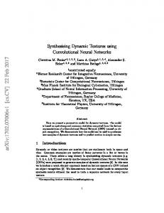
4. Experimental Results and Evaluation In Figure 1, one can see the performance over time of the reconstruction loss of the overall network. Notice how the loss approaches and then passes the loss value of 1 (which is the worst possible loss value not considering the regularization term for sparsity). Over time, the network is learning to restrict its receptive fields to spatial locations while also searching for optimal spots in the network to produce critical Ising patterns.

25

Reconstruction Loss

20

15

10

5

0

0

50

100

150 200 250 Fine Tuning Iteration

300

350

400

Figure 1: There is a steady decline and eventual convergence in the reconstruction loss for LargeNet. The parameters I used were `1 = 5 × 10−4 , minibatch size of 100, number of epochs of 400.

In Figure 2, one can see the visualization for the reconstruction by the RBM of critical point Ising models generated at T = Tc for the Ising Model. Notice that the reconstruction is very smooth, reminiscent of convolutional behavior and much simpler to encode in the RBM than a noisy pattern. It is this encoding that lies at the center of both convolutional neural nets in generation tasks [6] and transformation to variational space in statistical mechanics. 6

Reconstructed

Actual

Reconstructed

Actual

Reconstructed

Actual

Reconstructed

Actual

Figure 2: [Left] SmallNet. [Right] LargeNet reconstructions for the same two test examples show similarity in structure but differences in resolution.

In Figure 3, one can see the visualization of the neural network receptive fields for layers 0-2 for LargeNet and 0-1 for SmallNet, attempting to replicate ˆ the Qi results in [1]. More formally, the receptive field is defined as Wi = k=0 Wi , representing the feed-forward total weights of the hidden layer as calculated starting from the visible node region to that given layer. Note that in the network, the weights are defined as Wi for layer i and biases are defined as bi for layer i. In the visualization we notice that the receptive fields are not scattered and rather they tend to focus on spatial locations of the mask, particularly for LargeNet because it was trained for a much longer time than SmallNet. In summary, LargeNet is much less noisy than SmallNet thanks to training and finer resolution in convolution. Also in the visualization, notice that there is an interesting phenomenon: receptive fields do not belong to their own windows as they do in [1], but rather, multiple receptive regions are observed in a single local group of activations stemming from a single neuron. This should not be due to the fact that the network was still not fully trained because the `1 loss would have prevented the dead neurons (where there is no receptive field) from coming alive again. It is possible, however, that differences in `1 regularization magnitude (I used 5 × 10−4 instead of 2 × 10−4 as was done in [1]) led to lower ability to recover dead neurons during training and some of the other neurons had to make up for the deficit of the dead neurons in the network. Through the exercise, one may recognize several potential problems with learning receptive fields that replicate the paper. Firstly, employing `1 regularization is absolutely necessary. There are 7

Figure 3: Visualizations of receptive fields for [Top] SmallNet (using hot colormap), W0 and W1 left to right. [Bottom] LargeNet, W1 and W2 left to right. I used a prism colormap to put special emphasis on some of the patterns in the receptive fields including the fact that there are dead neurons.

several ways for the weights in the network to produce the patterns of the same Ising input, i.e. many combinations of weight matrix values work to produce the same encoding since there is information degeneracy in the network. A simple example of this is for a fully ordered Ising lattice. Multiple weight matrices (stemming from any ’on’ neuron to the visible layer) could be uniformly activated to make that pattern. However, since the `1 norm helps to enforce sparse patterns, we end up with results closer to what we would expect (mimicking receptive fields of convolutional neural networks). Secondly, training the network is rather difficult because the natural tendency for the DBN is to be lazy and set all of its reconstruction outputs close to zero (ending up with a mean-squared loss around 1). This experiment suffered from many of these issues, leading to weights that weren’t as nice as those in [1], but still showed limited receptive regions as expected for a convolutional application. Strangely, only visible nodes with Gaussian noise 8

worked (the usual binary assignments led to an exploding gradient during training), which is why we have smooth reconstruction profiles rather than discrete binary ones. The main takeaway from this exercise is that receptive fields are spatially constrained when presented with the Ising model samples, and the behavior is reminiscent of singling out blocks of spins and encoding them into simpler representations. Because the Hamiltonian of parametrized variational space is equivalent to the Boltzmann machine in that same variational space, it makes sense that this behavior continues in a stacked manner, and in every layer, we move into a new learned manifold via block renormalization with the hidden layer as our new ”visible layer.” 5. Conclusion We have demonstrated how to construct convolutional net-like structures from a deep belief network using Ising models, which shows the powerful connections of statistical mechanics theory and deep learning. Due to [1], we also have shown that there is a one-to-one mapping that allows for convolutional net-like structures to be constructed. Deep nets perform variational renormalization with every layer transformation, leading to automated evolution of structured feature design. Such new intuition suggests that deep learning and perception have applications rooted in theoretical physics ideas. Further investigation of physics renormalization groups may lead to similar revelations about other neural network structures, such as fixed point analysis of recurrent connections. There are still many answers needed such as what are the neural activations like at the end of the blocked spin funnel in the RBM? Is there an explicit symmetry breaking phenomenon during the learning process and how can we detect it? With the prospect of further investigation into our experimental results and into more neural architectures with the renormalization perspective, there is still much to learn at the interface of physics and AI. [1] P. Mehta, D. J. Schwab, An exact mapping between the variational renormalization group and deep learning, arXiv preprint arXiv:1410.3831 (2014). [2] L. P. Kadanoff, A. Houghton, M. C. Yalabik, Variational approximations for renormalization group transformations, Journal of Statistical Physics 14 (1976) 171–203. 9

[3] T. Mora, W. Bialek, Are biological systems poised at criticality?, Journal of Statistical Physics 144 (2011) 268–302. [4] P. Bak, C. Tang, K. Wiesenfeld, Self-organized criticality: An explanation of the 1/f noise, Physical review letters 59 (1987) 381. [5] U. Wolff, Collective monte carlo updating for spin systems, Physical Review Letters 62 (1989) 361. [6] J. Masci, U. Meier, D. Cire¸san, J. Schmidhuber, Stacked convolutional auto-encoders for hierarchical feature extraction, in: Artificial Neural Networks and Machine Learning–ICANN 2011, Springer, 2011, pp. 52– 59.

10