Convolutional Neural Networks on Non-Euclidean ... - Semantic Scholar

ShapeNet: Convolutional Neural Networks on Non-Euclidean Manifolds Jonathan Masci†∗

Davide Boscaini†∗

Michael M. Bronstein†

Pierre Vandergheynst‡

†

‡

Universit`a della Svizzera Italiana (USI), Lugano, Switzerland Ecole Polytechnique F´ed´erale de Lausanne (EPFL), Lausanne, Switzerland

max

...

...

Σ f1out

filter bank 2

max

...

f2out

...

...

f2in = g2

...

Σ

...

...

ξ

Σ

...

Σ

...

filter bank Q

in = g fM M

Input layer M -dim

Fully connected layer

ReLU layer

max Σ

...

...

ξ

Σ

...

Σ

...

arXiv:1501.06297v1 [cs.CV] 26 Jan 2015

f1in = g1

Σ

...

ξ

...

Σ

Nθ rotations

filter bank 1 P filters

Geodesic convolutional layer

out fQ

AMP layer

Output layer Q-dim

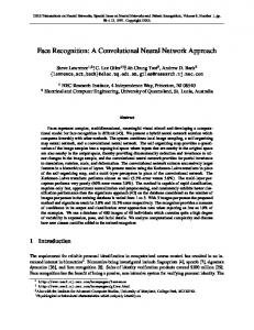
Figure 1: ShapeNet applied to M = 150-dimensional geometry vectors (input layer) of a human shape, to produce a Q = 16-dimensional feature descriptor (output layer). The neural network shown here is a simple configuration consisting of a fully connected (FC) layer, a ReLU layer applying the non-linear function ξ, a geodesic convolutional (GC) layer with Q filter banks consisting of P filters each. Convolutions are performed in local geodesic polar coordinates; each filter is applied for all Nθ possible rotations. Finally, to remove the rotation ambiguity, angular max pooling (AMP) is applied. See text for details.

Abstract

1

Feature descriptors play a crucial role in a wide range of geometry analysis and processing applications, including shape correspondence, retrieval, and segmentation. In this paper, we propose ShapeNet, a generalization of the popular convolutional neural networks (CNN) paradigm to non-Euclidean manifolds. Our construction is based on a local geodesic system of polar coordinates to extract “patches”, which are then passed through a cascade of filters and linear and non-linear operators. The coefficients of the filters and linear combination weights are optimization variables that are learned to minimize a task-specific cost function. We use ShapeNet to learn invariant shape feature descriptors that significantly outperform recent state-of-the-art methods, and show that previous approaches such as heat and wave kernel signatures, optimal spectral descriptors, and intrinsic shape contexts can be obtained as particular configurations of ShapeNet.

Feature descriptors are a ubiquitous tool in shape analysis. Broadly speaking, a feature descriptor assigns to each point (or a subset of points) on the shape a vector in some multi-dimensional descriptor space representing the local structure of the shape around that point. Local feature descriptors are used in higher-level tasks such as establishing correspondence between shapes [Ovsjanikov et al. 2012], shape retrieval [Mitra et al. 2006; Bronstein et al. 2011], or segmentation [Skraba et al. 2010]. The construction of descriptors is largely application dependent, and one typically tries to make the descriptor discriminative (capture the structures that are important for a particular application, e.g. telling apart two classes of shapes), robust (invariant to some class of transformations or noise), compact (in the sense of low dimensionality of the descriptor space), and computationally-efficient.

CR Categories: I.2.6 [Artificial Intelligence]: Learning— Connectionism and neural nets

Previous work

Keywords: Deep Learning, Convolutional Neural Networks, Shape Descriptors ∗ equal

contribution

Introduction

Early works on shape descriptors such as spin images [Johnson and Hebert 1999], shape distributions [Osada et al. 2002], integral volume descriptors [Manay et al. 2006], and multiscale features [Pauly et al. 2003] were based on extrinsic structures that are invariant under Euclidean transformations. The following generation of shape descriptors used intrinsic structures such as geodesic distances [Hamza and Krim 2003; Elad and Kimmel 2003]

or conformal factor [Ben-Chen and Gotsman 2008]. The success of image descriptors such as Harris operator [Harris and Stephens 1988], SIFT [Lowe 2004], HOG [Dalal and Triggs 2005], MSER [Matas et al. 2004], and shape context [Belongie et al. 2000] has led to several generalizations thereof to non-Euclidean domains (see e.g. [Sipiran and Bustos 2011; Zaharescu et al. 2009; Digne et al. 2010; Litman et al. 2011; Kokkinos et al. 2012], respectively). The pioneering works of [B´erard et al. 1994; Coifman and Lafon 2006; L´evy 2006; Rustamov 2007] on diffusion and spectral geometry have led to the emergence of intrinsic spectral shape descriptors that are invariant to isometric deformations of the shape and are dense, i.e. can be computed at every point of the shape. Notable examples in this family include heat kernel signatures (HKS) [Sun et al. 2009; Gebal et al. 2009], their scale-invariant version [Bronstein and Kokkinos 2010], and wave kernel signatures (WKS) [Aubry et al. 2011]. Arguing that in many cases it is hard to model invariance but rather easy to create examples of similar and dissimilar shapes, Litman and Bronstein [2014] showed that HKS and WKS can be considered as particular parametric families of transfer functions applied to the Laplace-Beltrami operator eigenvalues and proposed to learn an optimal transfer function. Their work follows the recent trends in the image analysis domain, where hand-crafted descriptors are abandoned in favor of learning approaches. The past decade in computer vision research has witnessed the re-emergence of “deep learning” and in particular, convolutional neural network (CNN) techniques allowing to learn task-specific features from examples. Though originated already in the 1980s [Fukushima 1980; LeCun et al. 1989], the availability of very large training datasets as well as computational power allowing to train deep models with many layers has enabled a breakthrough in performance in a wide range of applications such as image classification [Krizhevsky et al. 2012; Papandreou et al. 2014], segmentation [Ciresan et al. 2012], detection and localization [Sermanet et al. 2014; Simonyan and Zisserman 2014] and annotation [Fang et al. 2014; Karpathy and Fei-Fei 2014]. The main strength of CNN is the ability to learn hierarchical abstractions from large collections of data, thus requiring very little task-specific prior knowledge. Unfortunately, in the 3D shape analysis community, deep learning methods are practically unused, with a few recent exceptions such as application of random forests for shape correspondence [Shotton et al. 2013; Rodol`a et al. 2014] and learning of bag-of-word descriptors by supervised sparse coding [Litman et al. 2014]. In the signal processing community, there have been several recent works on performing learning on graphs [Rustamov and Guibas 2013; Thanou et al. 2014]. One of the key reasons that so far have precluded the adoption of CNNs and similar methods in shape analysis is that unlike images that can be modeled as shift-invariant spaces, 3D shapes are typically represented as Riemannian manifolds (surfaces) on which there is no shift invariance, and hence the notion of convolution does not exist in the classical sense. In a recent work, Bruna et al. [2014] proposed a spectral formulation of CNNs on graphs using the notion of generalized (non shift-invariant) convolution. Their formulation relies on the analogy between the classical Fourier transform and the Laplace-Beltrami eigenbasis, and the fact that the convolution operator is diagonalized by the Fourier transform (or in other words, convolution in space corresponds to multiplication in frequency) [Shuman et al. 2013]. The main drawback of this approach is that while it allows to extend CNNs to a non-Euclidean domain, it does not allow applying the same model across different domains, since the convolution coefficients are expressed in a specific basis that is domain-dependent. As a result, a CNN that is trained on one shape cannot be applied to another shape, which limits the practical

applicability of such a method in the shape analysis field. In this paper, we propose ShapeNet, an extension of convolutional neural networks to non-Euclidean manifolds, and show its use in the construction of invariant shape descriptors. ShapeNet uses a local system of geodesic polar coordinates [Kokkinos et al. 2012] to extract “patches”, which are then passed through a cascade of filters and linear and non-linear operators. The parameters of these filters are optimization variables that are learned to minimize a task-dependent loss function. The framework is extremely flexible and by combining several layers with different configurations one can obtain different descriptors depending on the application in mind. Contribution

We see the following main contributions of our paper: first, in the domain of shape analysis, to the best of our knowledge, ShapeNet is the first extension of the CNN paradigm to non-Euclidean domains that is generalizable, i.e., it can be trained on one set of shapes and then applied to another one (as opposed to [Bruna et al. 2014]). Second, we show that HKS [Sun et al. 2009], WKS [Aubry et al. 2011], optimal spectral descriptors [Litman and Bronstein 2014], and intrinsic shape context [Kokkinos et al. 2012] can be obtained as particular configurations of ShapeNet; therefore, our approach is a generalization of previous approaches. Third, we show that ShapeNet descriptors achieve state-of-the-art performance on several challenging synthetic and real datasets. Fourth, while polar patches and the use of Fourier transform magnitude to obtain rotational invariance have been explored for the construction of hand-crafted image descriptors [Kokkinos and Yuille 2008], this has never been done before in the context of deep learning. The rest of the paper is organized as follows. In Section 2, we overview the basics of harmonic analysis on manifolds and the construction of popular spectral shape descriptors. Section 3 is dedicated to our construction of convolutional neural networks on manifolds. Section 4 presents experimental results. Section 5 discusses the limitations and possible extensions of our approach and concludes the paper. Organization

2 2.1

Background Main notions

We model a 3D shape as a connected smooth compact two-dimensional manifold (surface) X, possibly with a boundary ∂X. Locally around each point x the manifold is homeomorphic to a two-dimensional Euclidean space known as the tangent plane and denoted by Tx X. A mapping between the manifold and the tangent plane is established by the exponential map expx : Tx X → X. A Riemannian metric is an inner product h·, ·iTx X : Tx X ×Tx X → R on the tangent space depending smoothly on x. Manifold

We denote by L2 (X) the space of square-integrable real functions on X and by hf, giL2 (X) = R f (x)g(x)dx the standard inner product on L2 (X), where dx X is the infinitesimal area element induced by the Riemannian metric. Given a smooth function f ∈ L2 (X), we can define a function f ◦ expx : Tx X → R on the tangent plane. The Laplace-Beltrami operator (LBO) is a positive semidefinite operator ∆X : L2 (X) → L2 (X) defined as Laplace-Beltrami operator (LBO)

∆X f (x)

=

∆(f ◦ expx )(0),

(1)

where ∆ is the Euclidean Laplacian operator on the tangent plane.1 The LBO is intrinsic, i.e., expressible entirely in terms of the Riemannian metric. As a result, it is invariant to isometric (metricpreserving) deformations of the manifold. The LBO of a compact manifold admits an eigendecomposition ∆X φk = λk φk with a countable set of real eigenvalues 0 = λ1 ≤ λ2 ≤ . . . and the corresponding eigenfunctions φ1 , φ2 , . . . form an orthonormal basis on L2 (X). This basis is a generalization of the Fourier basis to non-Euclidean domains:2 given a function f ∈ L2 (X), it can be represented as the Fourier series X f (x) = hf, φk iL2 (X) φk (x), (2) Spectral analysis on manifolds

k≥1

where the analysis αk = hf, φk iL2 (X) can P be regarded as the forward Fourier transform and the synthesis k≥1 αk φk (x) is the inverse one; the eigenvalues {λk }k≥1 play the role of frequencies. The generalized convolution of f and g on the manifold can be defined by analogy to the classical case [Shuman et al. 2013] as the inverse transform of the product of forward transforms, X (f ? g)(x) = hf, φk iL2 (X) hg, φk iL2 (X) φk (x), (3) k≥1

and is in general non-shift-invariant (in the classical case, shift invariance is the result of associativity of the product of complex exponential functions). Heat diffusion on manifolds

is governed by the diffusion equa-

tion,  ∆X +

∂ ∂t

 u(x, t) = 0; u(x, 0) = u0 (x),

(4)

where u(x, t) denotes the amount of heat at point x at time t, u0 (x) is the initial heat distribution, and if the manifold has a boundary, appropriate boundary conditions must be added. The solution of (4) is obtained by applying the heat operator H t = e−t∆X to the initial condition, Z u(x, t) = H t u0 (x) = u0 (x0 )ht (x, x0 )dx0 , (5) X 0

In the discrete setting, the surface X is sampled at N points x1 , . . . , xN . On these points, we construct a triangular mesh (V, E, F ) with vertices V = {1, . . . , N }, in which each interior edge ij ∈ E is shared by exactly two triangular faces ikj and jhi ∈ F , and boundary edges belong to exactly one triangular face. The set of vertices {j ∈ V : ij ∈ E} directly connected to i is called the 1-ring of i. Discretization

A real function f : X → R on the surface is sampled on the vertices of the mesh and can be identified with an N -dimensional vector f = (f (x1 ), . . . , f (xN ))> . The discrete version of the LBO is given as an N × N matrix L = A−1 W, where   (cot Pαij + cot βij )/2 ij ∈ E; − k6=i wik i = j; wij = (7)  0 else; αij , βij denote the angles ∠ikj, ∠jhi of the triangles P sharing the edge ij, and A = diag(a1 , . . . , aN ) with ai = 31 jk:ijk∈F Aijk being the local area element at vertex i and Aijk denoting the area of triangle ijk [Pinkall and Polthier 1993; Meyer et al. 2003]. The first K ≤ N eigenfunctions and eigenvalues of the LBO operator are computed by performing the generalized eigendecomposition WΦ = AΦΛ, where Φ = (φ1 , . . . , φK ) is an N × K matrix containing as columns the discretized eigenfunctions and Λ = diag(λ1 , . . . , λK ) is the diagonal matrix of the corresponding eigenvalues.

2.2

Spectral descriptors

Sun et al. [2009] and Gebal et al. [2009] proposed a construction of intrinsic dense descriptors by considering the diagonal of the heat kernel, X −tλ 2 ht (x, x) = e k φk (x), (8) Heat Kernel Signature (HKS)

k≥0

also known as the autodiffusivity function. The physical interpretation of autodiffusivity is the amount of heat remaining at point x after time t. Geometrically, autodiffusivity is related to the Gaussian curvature K(x) by virtue of the Taylor expansion 1 ht (x, x) = 4πt + K(x) + O(t). Sun et al. [2009] defined the heat 12π kernel signature (HKS) of dimension Q at point x by sampling the autodiffusivity function at some fixed times t1 , . . . , tQ ,

where ht (x, x ) is known as the heat kernel. Since H t has the same eigenfunctions as ∆X with the eigenvalues {e−tλk }k≥1 , we can express the solution of (4) in the Fourier domain as X u(x, t) = H t u0 (x) = hu0 , φk iL2 (X) e−tλk φk (x) (6) k≥1

Z = X

u0 (x0 )

X

e−tλk φk (x)φk (x0 ) dx0 ,

k≥1

|

{z

ht (x,x0 )

}

allowing to interpret the heat kernel as the impulse response to a delta function at x0 . Furthermore, note that (6) has the generalized convolution form (3), where τ (λ) = e−tλ plays the role of a transfer function corresponding to a low-pass filter sampled at frequencies {λk }k≥1 . 1 Note

that contrary to many references, we consider the Laplacian with negative sign to have it positive semi-definite. 2 It is easy to verify that the classical Fourier basis functions eiωx are d2 iωx eigenfunctions of the Euclidean Laplacian operator − dx = ω 2 eiωx . 2e

f (x)

=

(ht1 (x, x), . . . , htQ (x, x))> .

(9)

The HKS has become a very popular approach in numerous applications due to several appealing properties. First, it is intrinsic and hence invariant to isometric deformations of the manifold by construction. Second, it is dense. Third, the spectral expression (8) of the heat kernel allows efficient computation of the HKS by using the first few eigenvectors and eigenvalues of the Laplace-Beltrami operator. At the same time, a notable drawback of HKS stemming from the use of low-pass filters is poor spatial localization (by the uncertainty principle, good localization in the Fourier domain results in a bad localization in the spatial domain). Aubry et al. [2011] considered a different physical model of a quantum particle on the manifold, whose behavior is governed by the Schr¨odinger equation,   ∂ i∆X + ψ(x, t) = 0, (10) ∂t Wave Kernel Signature (WKS)

where ψ(x, t) is the complex wave function capturing the particle behavior. Assuming that the particle oscillates at frequency λ drawn from a probability distribution π(λ), the solution of (10) can be expressed in the Fourier domain as X iλ t ψ(x, t) = e k π(λk )φk (x). (11) k≥1

The probability of finding the particle at point x is given by Z T X 2 p(x) = lim |ψ(x, t)|2 dt = π (λk )φ2k (x), (12) T →∞

0

k≥1

and depends on the initial frequency distribution π(λ). Aubry et al. [2011] considered a log-normal frequency distribution πν (λ) =
λ exp log ν−log with mean frequency ν and standard deviation σ. 2σ 2 They defined the Q-dimensional wave kernel signature (WKS) f (x)

=

(pν1 (x), . . . , pνQ (x))> ,

(13)

where pν (x) is the probability (12) corresponding to the initial log-normal frequency distribution with mean frequency ν, and ν1 , . . . , νQ are some logarithmically-sampled frequencies. While resembling the HKS in its construction and computation, WKS is based on log-normal transfer functions that act as band-pass filters and thus exhibits better spatial localization. Litman and Bronstein [2014] considered a generic Q-dimensional spectral descriptor given by a bank X f (x) = τ (λk )φ2k (x) (14) Optimal spectral descriptors (OSD)

2.3

Convolutional neural networks

In the field of computer vision, convolutional neural networks have become in the recent years one of the most powerful tools for image recognition and processing and have set a de-facto standard in the academia and industry on a variety of application. While many variants of CNNs have been proposed [Fukushima 1980; Riesenhuber and Poggio 1999] during the years, the most popular model is the one pioneered by LeCun et al. [1989], which allows gradientbased learning. The key ingredient of this successful model is the alternation of convolutional layers (applying a bank of filters on the input image), max-pooling layers (non-linear averaging operation) and fully connected layers (performing linear combination of inputs followed by a non-linear activation function acting as dimensionality reduction to the desired output dimension) to create a deep hierarchical processing pipeline. Thinking of an image as a function defined on the plane, due to shiftinvariance the convolution can be thought of as passing a template across the plane and recording the correlation of the template with the function at that location. The convolutional layer is parametrized by the coefficients of these templates (typically small e.g. 32 × 32 patches). One of the major problems in applying the CNN paradigm to non-Euclidean domains is the lack of shift-invariance, making it impossible to think of convolution as correlation with a fixed template: the template now has to be location-dependent.3 In an attempt to overcome this difficulty, Bruna et al. [2014] used the spectral generalization (3) of convolution. In this approach, the convolutional layer is specified in the Fourier domain,

Spectral CNN

k≥0

fqout (x)

>

of transfer functions τ (λ) = (τ1 (λ), . . . , τQ (λ)) . Both HKS and WKS can be considered as particular instances thereof: the former is obtained by using a family of low-pass transfer functions, while the latter is a family of band-pass ones. Litman and Bronstein [2014] use parametric transfer functions expressed as τq (λ)

=

M X

aqm βm (λ)

in some fixed (e.g. B-spline) basis β1 (λ), . . . , βM (λ), where aqm (q = 1, . . . , Q, m = 1, . . . , M ) are the parametrization coefficients. Plugging (15) into (14) one can express the qth component of the spectral descriptor as =

X k≥0

τq (λk )φ2k (x) =

M X m=1

aqm

X

βm (λk )φ2k (x),(16)

k≥0

|

P XX

αk,qp hfpin , φk iL2 (X) φk (x),

(17)

k≥1 p=1

where f in (x) = (f1in (x), . . . , fPin (x)) denotes the P -dimensional out layer input, f out (x) = (f1out (x), . . . , fQ (x)) is the Qdimensional layer output, and {αk,qp }k≥1 are the coefficients representing in the Fourier domain the pth filter in the qth filter bank.

(15)

m=1

fq (x)

=

{z

gm (x)

While allowing to extend CNNs to non-Euclidean domains, this formulation does not allow applying the model across different domains. The reason is that the filter spectral representation {αk }k≥1 is done with respect to the Laplace-Beltrami eigenbasis {φk }k≥1 , which is specific for the manifold X. Given another shape Y with a possibly different basis {ψk }k≥1 , the coefficients {αk }k≥1 learned on X cannot be applied on Y anymore. Thus, the Spectral CNN model cannot generalize to new, previously unseen shapes, making it impractical in shape analysis applications.

}

where g(x) = (g1 (x), . . . , gM (x))> is a vector-valued function referred to as geometry vector, dependent only on the intrinsic geometry of the shape. Thus, (14) is parametrized by the Q × M matrix A = (alm ) and can be written in matrix form as f (x) = Ag(x). The main idea of [Litman and Bronstein 2014] is to learn the optimal parameters A by minimizing a task-specific loss. Given a training set consisting of a pair of geometry vectors g, g+ representing knowingly similar points (positives), and g, g− representing knowingly dissimilar points (negatives), one tries to find A such that kf − f + k = kA(g − g+ )k is as small as possible and kf − f − k = kA(g − g− )k is as large as possible. The authors show that the problem boils down to a simple Mahalanobis-type metric learning.

3 3.1

Deep learning on manifolds Geodesic convolution

In this paper, we use a different notion of convolution on nonEuclidean domains that follows the ‘correlation with template’ idea by employing a local system of geodesic polar coordinates constructed at point x shown in Figure 2. The radial coordinate is constructed as ρ-level sets {x0 : dX (x, x0 ) = ρ} of the geodesic (shortest path) distance function for ρ ∈ [0, ρ0 ]; we call ρ0 the radius 3 If the manifold has continuous isometry group, e.g. rotation symmetry, it is still possible to think of convolution as passing a template; however, in practical applications shapes rarely have any continuous symmetry.

1

2

Nθ

3 4

x

Γ(x, θ)

θ x

8 5 7

6

vθ

vρ

Figure 2: Construction of local geodesic polar coordinates on a manifold. Left: examples of local geodesic patches, center and right: example of angular and radial weights vθ , vρ , respectively (red denotes larger weights). of the geodesic disc. 4 The angular coordinate is constructed as a set of geodesics Γ(x, θ) emanating from x in direction θ; such rays are perpendicular to the geodesic distance level sets. Note that the choice of the origin of the angular coordinate is arbitrary. For boundary points, the procedure is very similar, with the only difference that instead of mapping into a disc we map into a half-disc. Let Ω(x) : Bρ0 (x) → [0, ρ0 ] × [0, 2π) denote the bijective map from the manifold into the local geodesic polar coordinates (ρ, θ) around x, and let (D(x)f )(ρ, θ) = (f ◦ Ω−1 (x))(ρ, θ) be the patch operator interpolating f in the local coordinates. We can regard D(x)f as a ‘patch’ on the manifold and use it to define what we term the geodesic convolution (GC), (f ? a)(x) =

X

a(θ + ∆θ, r)(D(x)f )(r, θ),

(18)

θ,r

where a(θ, r) is a filter applied on the patch. Due to angular coordinate ambiguity, the filter can be rotated by arbitrary angle ∆θ. Patch operator

Kokkinos et al. [2012] construct the patch opera-

tor as Z (D(x)f )(ρ, θ)

vρ,θ (x, x0 )f (x0 )dx0 ,

=

(19)

X

where vρ,θ (x, x0 )

0

=

R

0

vρ (x, x )vθ (x, x ) v (x, x0 )vθ (x, x0 )dx0 X ρ

(20)

are interpolation weights. The radial weight is a Gaussian 0 2 2 vρ (x, x0 ) ∝ e−(dX (x,x )−ρ) /σρ of the geodesic distance from x, centered around ρ (see Figure 2, right). The angular weight is a 2 0 2 Gaussian vθ (x, x0 ) ∝ e−dX (Γ(x,θ),x )/σθ of the point-to-set dis0 tance dX (Γ(x, θ), x ) = minx00 ∈Γ(x,θ) dX (x00 , x0 ) to the geodesic Γ(x, θ) (see Figure 2, center). We stress this is only one possibility of constructing local coordinates and our model is not limited to this specific construction. 4 Rigorously speaking, only if the radius ρ of the geodesic ball 0 Bρ0 (x) = {x0 : dX (x, x0 ) ≤ ρ0 } is sufficiently small w.r.t the local convexity radius of the manifold, then the resulting ball is guaranteed to be a topological disc [Leibon and Letscher 2000]. Empirically, we see that choosing a sufficiently small ρ0 , e.g. 1% of the geodesic diameter diam(X) = maxx,x0 ∈X dX (x, x0 ) of the shape, produces valid topological discs. For larger values of ρ0 , at the points where the geodesic ball is not disc-like the radius can be reduced adaptively, or such points can be simply ignored. In the following, we tacitly assume Bρ0 (x) to be disc-like.

Figure 3: Construction of local geodesic polar coordinates on a triangular mesh. Shown clock-wise: division of 1-ring of vertex xi into Nθ equi-angular bins; propagation of a ray (bold line) by unfolding the respective triangles (marked in green). On triangular meshes, the construction of local geodesic patches is done according to [Kokkinos et al. 2012]. A discrete local system of coordinates has Nθ angular and Nρ radial bins. Starting with a vertex i, we first partition the 1-ring of i by Nθ rays into equi-angular bins, aligning the first ray with one of the edges (Figure 3). Next, we propagate the rays into adjacent triangles using an unfolding procedure resembling one used in [Kimmel and Sethian 1998], producing poly-lines that form the angular bins (see Figure 3). Radial bins are created as level sets of the geodesic distance function computed using fast marching [Kimmel and Sethian 1998]. Discrete patch operator

The discrete patch operator can be represented as a large matrix of size Nθ Nρ N × N applied to a function defined on the mesh vertices and producing the patches at each vertex. The matrix is very sparse since the values of the function at a few nearby vertices only contribute to each local geodesic polar bin, and thus the extraction of patches is computationally efficient and scales up to large meshes.

3.2

ShapeNet architecture

Using the notion of geodesic convolution, we are now ready to extend CNNs to manifolds. Our construction, referred to as ShapeNet, consists of several layers that are applied subsequently, i.e. the output of the previous layer is used as the input into the subsequent one (see Figure 1). The model is said to be deep if there are multiple “hidden” layers between the input and the output layers. We distinguish between the following types of layers: layer typically follows the input layer and precedes the output layer to adjust the input and output dimensions by means of a linear combination, Fully-connected (FC)

fqout (x)

=

P X

wqp fpin (x); q = 1, . . . , Q,

(21)

p=1

using notation as in (17). P Q coefficients wqp parametrize the FC layer. is a fixed layer applying the ReLU non-linear function ξ(t) = max{0, t} to each input dimension, ReLU

fpout (x)

=

ξ(fpin (x)); p = 1, . . . , P = Q.

(22)

layer replaces the convolutional layer used in classical Euclidean CNNs. Note that because of the angular coordinate ambiguity, we compute the geodesic convolution result for all Nθ rotations of the filters, Geodesic convolution (GC)

out f∆θ,q (x)

P X (fp ? a∆θ,qp )(x), q = 1, . . . , Q, (23)

=

p=1

where a∆θ,qp (θ, r) = aqp (θ + ∆θ, r) are the coefficients of the pth 2π θ −1) filter in the qth filter bank rotated by ∆θ = 0, N , . . . , 2π(N , Nθ θ and the convolution is understood in the sense of (18). The GC layer is parametrized by the coefficients of P Q filters, a total of Nθ Nρ P Q parameters. is a fixed layer used in conjunction with the GC layer, that computes the maximum over the filter rotations, Angular max-pooling (AMP)

fpout (x)

in max f∆θ,p (x), p = 1, . . . , P = Q,

=

∆θ

(24)

layer is another fixed layer that applies the patch operator to each input dimension, followed by Fourier transform w.r.t. the angular coordinate and absolute value, X out −iωθ in fp (ρ, ω) = e (D(x)fp (x))(ρ, θ) , (25) Fourier transform magnitude (FTM)

θ

p = 1, . . . , P = Q. The Fourier transform translates rotational ambiguity into complex phase ambiguity, which is removed by taking the absolute value [Kokkinos and Yuille 2008; Kokkinos et al. 2012].

Learning

The training of ShapeNet is implemented as a siamese neural network [Bromley et al. 1994; Hadsell et al. 2006], a popular architecture that has been widely used in metric learning problems [SimoSerra et al. 2014]. A siamese network is composed of two identical copies of the same model which share the same parameterization and are fed by pairs of knowingly similar or dissimilar samples. In our implementation, we minimize the following loss `(Θ) = (1 − γ)`+ (Θ) + γ`− (Θ),

(26)

where γ ∈ [0, 1] is a parameter trading off between the positive and negative losses, `+ (Θ)

`− (Θ)

=

=

|T+ | 1X i kFΘ (gi ) − FΘ (g+ )k2 , 2 i=0

3.4

(27)

|T− | 1X i max{0, µ − kFΘ (gi ) − FΘ (g− )k}2 ,(28) 2 i=0

FΘ denotes the ShapeNet model parameterized by Θ (all the parami eters in the GC and FC layers), and T± = {(gi , g± )} denote the sets of positive and negative pairs, respectively. The term (27) tries to map positive pairs as close as possible in the output space, while the term (28) pulls negative samples at a margin µ. Starting with a random set of parameters Θ, learning is performed by minimizing (26), making the ShapeNet learn the descriptor model

Relation to previous approaches

We note that several previous descriptors can be implemented as particular configurations of ShapeNet applied on geometry vectors input. HKS [Sun et al. 2009] and WKS [Aubry et al. 2011] descriptors are obtained by using a fixed FC layer configured to produce lowor band-pass filters, respectively. OSD [Litman and Bronstein 2014] is obtained by using an FC layer, whose parameters are learned. Intrinsic shape context [Kokkinos et al. 2012] is obtained by using a fixed FC layer configured to produce HKS or WKS descriptors, followed by a fixed FTM layer.

4 4.1

in where f∆θ,p is the output of the GC layer (23).

3.3

from the training data. After Θ is learned, the descriptors are computed by applying FΘ to input data. Given the exponential growth of the negative set, training of a siamese network is generally done on-line, using stochastic sampling methods to produce the input training pairs. We adopt the same strategy to train our ShapeNet.

Results Experiments setup

In this section, we evaluate the capability of ShapeNet in extracting feature descriptors following nearly-verbatim the experimental setup of [Litman and Bronstein 2014] so the reader can easily compare our results with previous works. The code of ShapeNet will be made available after the publication of the paper. We used three public-domain datasets: FAUST [Bogo et al. 2014] and SCAPE [Anguelov et al. 2005] datasets, containing scanned human shapes in different poses; and TOSCA [Bronstein et al. 2008] containing synthetic models of humans and animals in a variety of near-isometric deformations. For the latter we limited the evaluation to human shapes only to better compare with the other benchmarks. Amongst the three, the FAUST dataset is particularly challenging given a high variability of non-isometric deformations as well as significant variability between different human subjects. The meshes in TOSCA and SCAPE were resampled, respectively to 10K, 12.5K vertices whereas for FAUST we used the registration meshes without further pre-processing. We scaled all shapes to unit geodesic diameter. In FAUST and SCAPE datasets, groundtruth point-wise correspondence between the shapes was known; in TOSCA datasets, correspondence was known only between different poses of the same shape but not across shapes. Since we consider intrinsic descriptors, in all our evaluations we ignore intrinsic symmetry. Datasets

We compared the performance of the proposed ShapeNet to HKS [Sun et al. 2009], WKS [Aubry et al. 2011], and OSD [Litman and Bronstein 2014] using the code and settings provided by the respective authors. Laplace-Beltrami operators were discretized using the cotangent formula [Pinkall and Polthier 1993; Meyer et al. 2003]; K = 300 eigenfunctions were computed using MATLAB eigs function. To make the comparison fair, all the descriptors were Q = 16-dimensional as in [Litman and Bronstein 2014]. ShapeNet and OSD were trained on M = 150-dimensional geometry vectors computed according to (15)–(16) using B-spline bases. Methods and Settings

ShapeNet was implemented in Theano [Bergstra et al. 2010; Bastien et al. 2012] in two configurations: SN1 (150-dimensional input, FC layer with 16-dimensional output, ReLU layer, GC layer with 16-dimensional output, followed by AMP), and SN2 (same as SN1 with an additional ReLU layer, FTM layers, followed by a FC layer with 16-dimensional output); an example of intermediate computations in SN1 are shown in Figure 1. Local geodesic patches were

Near-isometric deformation

Non-isometric deformation

HKS

Topological noise

WKS

Geometric noise

Uniform Non-uniform subsampling subsampling

OSD

Missing parts

ShapeNet

Figure 4: Top: different shape transformations, shown left to right: two FAUST shapes in different poses, FAUST shape of a different person, SCAPE shape, TOSCA shape, topological noise (glued hands), additive Gaussian noise, uniform downsampling by 40%, non-uniform downsampling (the head, torso, and legs regions are downsampled by a different factor), missing parts. Bottom: 2D visualization (left to right) of the HKS, WKS, OSD, and ShapeNet descriptor space using t-SNE. Each point corresponds to a descriptor at a point on the shape marked in the respective color (ideally, points of same colors should form clusters that are as tight and as far apart as possible). generated using the code and settings of [Kokkinos et al. 2012]. The interpolation coefficients for all the points were pre-computed and stacked into an Nθ Nρ N × N sparse matrix; multiplication by such a matrix is efficient and scales up to very large meshes. Unless stated otherwise, the radius ρ0 of the geodesic patches was chosen as 1% of the geodesic shape diameter. Training Each dataset was split into disjoint training, validation, and test sets. On the FAUST dataset, we used subjects 1–7 for training, subject 8 for validation, and subject 9–10 for testing. On SCAPE, we used shapes 20–29 and 50–70 for training, five random shapes from the remaining ones for validation, and the rest for testing. On TOSCA, we test on all the deformations of the victoria shape.

The positive and negative sets of vertex pairs required for training were generated on the fly, having this way a very low memory and computational footprint, which makes feasible the usage of large scale datasets. Given that we have one-to-one correspondence between most of the shapes, the training pairs were constructed as follows: first, sample two shapes, then form the positive set with all corresponding points, and finally, form the negative set with first shape vertices and a random permutation of the ones of the second shape. This strategy differs from [Litman and Bronstein 2014] who considered only points on the same shape. The advantage of our sampling strategy is that it allows learning invariance also across several poses and subjects. We trained ShapeNet for a maximum of 2.5K updates (each update considering all points in the input shapes) using Adadelta [Zeiler 2012], which we found to converge much quicker than simple stochastic gradient descent with momentum. Typical training times on FAUST shapes were approximately 30 and 50 minutes for SN1 and SN2 models, respectively. Once trained, the application of a ShapeNet model to compute feature descriptors is very efficient: 75K and 45K vertices/sec for the SN1 and SN2 models, respectively. Timing

4.2

Descriptor performance

Figure 4 shows a two-dimensional visualization of ShapeNet descriptors computed at three points (knee, groin, and shoulder) across different shape transformations obtained using t-SNE dimensionality reduction [Van der Maaten and Hinton 2008]. An additional example of how the ShapeNet descriptors look like appears in Figure 1 (output layer). Descriptor visualization

Figures 5–6 (compare to Figure 2 in [Litman and Bronstein 2014]) depicts the Euclidean distance in the descriptor space between the descriptor at a selected point and the rest of the points on the same shape as well as its transformations. ShapeNet descriptors manifest both good localization (better than HKS) and discriminativity (less spurious minima than WKS and OSD), as well as robustness to different kinds of noise (isometric and non-isometric deformations, geometric and topological noise, different sampling, and missing parts). Similarity map

Descriptor evaluation Following [Litman and Bronstein 2014], we evaluated the descriptor performance using the cumulative match characteristic (CMC) and the receiver operator characteristic (ROC). The CMC evaluates the probability of a correct correspondence among the k nearest neighbors in the descriptor space. The ROC measures the percentage of positives and negatives pairs falling below various thresholds of their distance in the descriptor space (true positive and negative rates, respectively). Figure 7 shows the performance of different descriptors in terms of CMC and ROC characteristics on the FAUST and SCAPE datasets. We observe that ShapeNet descriptors significantly outperform other descriptors, and that the more complex model (SN2) further boosts performance. Table 1 reports the equal error rate (EER), defined as the intersection point of the false positive and false negative rate curves. Lower values indicate better discriminativity of the descriptors.

Heat kernel signature (HKS)

Wave kernel signature (WKS)

Optimal spectral descriptor (OSD)

ShapeNet

Figure 5: Normalized Euclidean distance between the descriptor at a reference point on the shoulder (marked in white circle) and HKS, WKS, OSD and ShapeNet descriptors (first to fourth rows, respectively) computed at the rest of the points on different transformations of the leftmost shape. Transformations are the same as in Figure 4. Cold and hot colors represent small and large distances, respectively; for visualization purpose, the distances are saturated at the median distance. Train Test HKS WKS OSD SN1 SN2 FAUST FAUST 12.02 12.46 8.74 5.21 4.04 SCAPE SCAPE 6.43 17.94 12.22 3.43 3.34 FAUST TOSCA 4.18 8.98 8.91 6.63 5.61 Table 1: Equal error rate (EER %) performance of the various descriptors on intra- and inter-dataset (transfer) matches. Note that HKS and WKS are not learned descriptors.

In order to test the generalization capability of the learned descriptors, we applied OSD and ShapeNet learned on the FAUST dataset to TOSCA shapes. Figure 8 visualizes the respective ROC and CMC curves. We see that the learned model transfers well to a new dataset and that ShapeNet outperforms other descriptors. Generalization capability

positive and negative pairs in the training set, with larger values of γ resulting in a better localization. Finally, using a larger patch radius ρ0 improves performance, however, at the expense of having a denser patch operator matrix, which impacts the training times.

4.3

Correspondence

In our final set of experiments, we use the descriptors to find correspondence between shapes. We stress that these results should by no means be compared to state-of-the-art correspondence methods, but rather considered as a way of assessing the quality of feature descriptors and to show that ShapeNet allows obtaining high-quality correspondence even when used in a na¨ıve way. In this evaluation, each point is assigned to its nearest neighbor in the descriptor space, thus avoiding bias towards a particular matching method (only the quality of the raw descriptors is considered). Figure 10 evaluates the resulting correspondence using the Princeton protocol [Kim et al. 2011], plotting the percentage of matches that are at most r-geodesically distant from the groundtruth correspondence. ShapeNet (used in the SN2 configuration) achieves the best performance among the Nearest-neighbor correspondence

To test the influence of different parameters, we used the SN1 configuration of ShapeNet with different values of training parameters γ and µ, and different geodesic patch radii ρ0 . Figure 9 shows the performances evaluation on the FAUST dataset. Higher margin µ results in better performance, however, the effect is not very significant. Varying γ allows to trade off between Influence of parameters

Heat kernel signature (HKS)

Wave kernel signature (WKS)

Optimal spectral descriptor (OSD)

ShapeNet

Figure 6: Normalized Euclidean distance between the descriptor at a reference point on the groin (marked in white circle) and HKS, WKS, OSD and ShapeNet descriptors (first to fourth rows, respectively) computed at the rest of the points on different transformations of the leftmost shape. Transformations are the same as in Figure 4. Cold and hot colors represent small and large distances, respectively; for visualization purpose, the distances are saturated at the median distance. compared descriptors. We repeat the experiment of Litman and Bronstein [2014], in which each of one hundred points sampled on one shape are matched to 20 nearest candidate points on the other shape using the Euclidean distance in the descriptor space; the resulting affinity matrix is then fed into the spectral correspondence algorithm [Leordeanu and Hebert 2005] to obtain a point-to-point correspondence between the shapes. Figure 11 shows “good” correspondences (falling within a geodesic ball of radius equal to 10% of the geodesic shape diameter around the groundtruth corresponding point) obtained by spectral matching based on different descriptors (compare to to Figure 3 in [Litman and Bronstein 2014]). We observe that ShapeNet produces the largest number of good correspondences. Spectral matching

Functional correspondence Following [Ovsjanikov et al. 2012], we estimate a linear operator T : L2 (X) → L2 (Y ) representing the functional correspondence between shapes X and Y in the Fourier domain,

Tf =

K X p,q=1

cpq hf, φp iL2 (X) ψq ,

(29)

from a set of knowingly corresponding functions on X and Y . In our case, we used K = 20 and sampled fifty points on X using farthest point sampling [Hochbaum and Shmoys 1985] and found the corresponding points on Y using the closest matches in the descriptor space; the indices of the corresponding points are denoted by i1 , . . . , i50 and j1 , . . . , j50 , respectively. By solving the linear system of equations ψq (yjl )

=

K X

cpq φp (xil ), l = 1, . . . , 50

(30)

p=1

in the least-squares sense, the K × K matrix C = (cpq ) translating the Fourier coefficients between the bases {φk }k≥1 and {ψk }k≥1 is recovered, allowing to map a function from X to Y according to (29). Figure 12 shows examples of functional correspondence obtained using OSD and ShapeNet (in SN2 configuration) descriptors; the proposed method results in a significantly better correspondence.

5

Conclusions

In this paper, we presented ShapeNet, a generalization of convolutional neural networks allowing to learn hierarchical task-specific

FAUST-FAUST

FAUST-FAUST 1

0.9

0.9

0.8

0.8

0.7

0.7

True Positive Rate

1

Hit rate

0.6 0.5 0.4

0.6 0.5 0.4 0.3

0.3 HKS WKS OSD SN1 SN2

0.2 0.1

0.1 0 10 -3

0 0

10

20

30

40

50

60

70

80

90

HKS WKS OSD SN1 SN2

0.2

100

Number of matches

10 -2

SCAPE-SCAPE

10 0

SCAPE-SCAPE 1

0.9

0.9

0.8

0.8

0.7

0.7

True Positive Rate

1

0.6

Hit rate

10 -1

False Positive Rate

0.5 0.4 0.3

0.6 0.5 0.4 0.3

HKS WKS OSD SN1 SN2

0.2 0.1

0.1

0 0

10

20

30

40

50

60

70

80

90

HKS WKS OSD SN1 SN2

0.2

0 10 -3

100

Number of matches

10 -2

10 -1

10 0

False Positive Rate

Figure 7: Performance of different descriptors measured using the CMC (left) and ROC (right) on FAUST (top) and SCAPE (bottom) datasets. In both cases, training and testing were performed on disjoint sets of the same datasets. ShapeNet (red and blue curves) significantly outperforms other descriptors. FAUST-TOSCA

FAUST-TOSCA 1

0.9

0.9

0.8

0.8

0.7

0.7

True Positive Rate

1

Hit rate

0.6 0.5 0.4 0.3

0.6 0.5 0.4 0.3

HKS WKS OSD L1 L2

0.2 0.1

0.1

0 0

10

20

30

40

50

60

Number of matches

70

80

90

HKS - eer=4.18% WKS - eer=8.98% OSD - eer=8.91% L1 - eer=6.63% L2 - eer=5.61%

0.2

100

0 10 -3

10 -2

10 -1

10 0

False Positive Rate

Figure 8: Example of generalization of descriptors learned on FAUST shapes and tested on TOSCA. Performance is measured using the CMC (left) and ROC (right) characteristics. (HKS and WKS are not learned descriptors and are shown here for reference only).

1

0.9

0.9

0.8

0.8

0.7

0.7

0.6

0.6

Hit rate

Hit rate

1

0.5 µ=1, γ=0.75, ρ0 =1% µ=5, γ=0.25, ρ0 =1%

0.4

0.3

µ=5, γ=0.75, ρ0 =1% µ=50, γ=0.75, ρ0 =1%

0.2

0.2

µ=5, γ=0.75, ρ0 =2% µ=5, γ=0.75, ρ0 =10%

0.1

0.5 0.4

µ=5, γ=0.50, ρ0 =1%

0.3

FAUST

HKS WKS OPT SN2

0.1 0

0 0

10

20

30

40

50

60

70

80

90

0

100

0.05

0.1

0.15

0.2

0.25

Geodesic Radius

Number of matches

1

0.8

0.9

0.7

SCAPE

0.8

0.5 0.6

Hit rate

True Positive Rate

0.6 0.7

0.5 µ=1, γ=0.75, ρ0 =1% µ=5, γ=0.25, ρ0 =1% µ=5, γ=0.50, ρ0 =1%

0.4 0.3 0.2 0.1 0 10 -3

0.4

0.3

µ=5, γ=0.75, ρ0 =1%

0.2

µ=50, γ=0.75, ρ0 =1% µ=5, γ=0.75, ρ0 =2%

0.1

HKS WKS OPT SN2

µ=5, γ=0.75, ρ0 =10% 0 10 -2

10 -1

10 0

0

0.05

0.1

Figure 9: Influence of the parameters (geodesic disc radius ρ0 , margin µ, and positive/negative loss weight γ) on ShapeNet performance tested on the FAUST dataset. Shown are CMC (top) and ROC (bottom) plots. features on non-Euclidean manifolds. The model is very generic and flexible, and can be made arbitrarily complex by stacking multiple layers. Furthermore, our model generalizes several previous shape descriptor methods (HKS, WKS, optimal spectral descriptors, and intrinsic shape contexts) and achieves better performances than any of these descriptor we tested in our experiments. Speaking more broadly, we believe that our work shows the power of deep learning methods on manifolds, and we hope it will lead to followup works exploring other successful learning models. Our current ShapeNet implementation uses a construction of local geodesic coordinates that is specific for triangular meshes, hence our experiments were so far limited to meshes only. However, the model itself is rather generic, and can be applied to other shape representations such as point clouds; provided an alternative local charting technique. In future works, we plan to explore other more generic constructions of local coordinates that can be used not only on surfaces but also on graphs. Furthermore, in this paper we considered geometric descriptors where the input to the network is constituted of intrinsic spectral properties of the shape (in particular, we used geometry vectors). However, ShapeNet can be applied on any function defined on the manifold, and it would Limitations and Extensions

0.15

0.2

0.25

Geodesic Radius

False Positive Rate

Figure 10: Evaluation of nearest neighbor matching based on different descriptors using the Princeton protocol (shown is the percentage of matches falling within a geodesic ball of increasing radius around the groundtruth match).

HKS (16)

WKS (43)

OSD (46)

ShapeNet (64)

Figure 11: Spectral shape matching based on (left to right) HKS, WKS, OSD, and ShapeNet descriptors. Shown in green lines are “good” correspondences with geodesic error below 10% of shape diameter (the number of good correspondences appears in parenthesis).

be particularly natural to use it to construct descriptors of textured surfaces.

References A NGUELOV, D.,

ET AL .

2005. SCAPE: Shape completion and

C IRESAN , D. C., G IUSTI , A., G AMBARDELLA , L. M., AND S CHMIDHUBER , J. 2012. Deep neural networks segment neuronal membranes in electron microscopy images. In Proc. NIPS. C OIFMAN , R. R., AND L AFON , S. 2006. Diffusion maps. Applied and Computational Harmonic Analysis 21, 1, 5–30. OSD

DALAL , N., AND T RIGGS , B. 2005. Histograms of oriented gradients for human detection. In Proc. CVPR, vol. 1, 886–893. D IGNE , J., M OREL , J.-M., AUDFRAY, N., AND M EHDI -S OUZANI , C. 2010. The level set tree on meshes. In Proc. 3DPVT, vol. 2. E LAD , A., AND K IMMEL , R. 2003. On bending invariant signatures for surfaces. PAMI 25, 10, 1285–1295.

ShapeNet

Figure 12: Functional correspondence between a reference shape (leftmost column) and a few of its deformations using OSD (top) and ShapeNet (bottom) descriptors. Similar colors represent corresponding points. Third, fifth, and seventh columns depict the absolute value of matrices C of correspondence coefficients in the Fourier domain (brighter colors represent values closer to zero).

animation of people. TOG 24, 3, 408–416. AUBRY, M., S CHLICKEWEI , U., AND C REMERS , D. 2011. The wave kernel signature: A quantum mechanical approach to shape analysis. In Proc. ICCV, 1626–1633. BASTIEN , F., ET AL . 2012. Theano: new features and speed improvements. In Proc. Workshop on Deep Learning and Unsupervised Feature Learning. B ELONGIE , S., M ALIK , J., AND P UZICHA , J. 2000. Shape context: A new descriptor for shape matching and object recognition. In Proc. NIPS. B EN -C HEN , M., AND G OTSMAN , C. 2008. Characterizing shape using conformal factors. In Proc. 3DOR. B E´ RARD , P., B ESSON , G., AND G ALLOT, S. 1994. Embedding riemannian manifolds by their heat kernel. Geometric & Functional Analysis 4, 4, 373–398. B ERGSTRA , J., ET AL . 2010. Theano: a CPU and GPU math expression compiler. In Proc. SciPy.

FANG , H., ET AL . 2014. From captions to visual concepts and back. arXiv:1411.4952. F UKUSHIMA , K. 1980. Neocognitron: A self-organizing neural network model for a mechanism of pattern recognition unaffected by shift in position. Biological Cybernetics 36, 4, 193–202. G EBAL , K., B ÆRENTZEN , J. A., A NÆS , H., AND L ARSEN , R. 2009. Shape analysis using the auto diffusion function. CGF 28, 5, 1405–1413. H ADSELL , R., C HOPRA , S., AND L E C UN , Y. 2006. Dimensionality reduction by learning an invariant mapping. In Proc. CVPR. H AMZA , A. B., AND K RIM , H. 2003. Geodesic object representation and recognition. In Proc. DGCI. H ARRIS , C., AND S TEPHENS , M. 1988. A combined corner and edge detector. In Proc. Alvey Vision Conf. H OCHBAUM , D. S., AND S HMOYS , D. B. 1985. A best possible heuristic for the k-center problem. Mathematics of Operations Research 10, 2, 180–184. J OHNSON , A. E., AND H EBERT, M. 1999. Using spin images for efficient object recognition in cluttered 3D scenes. PAMI 21, 5, 433–449. K ARPATHY, A., AND F EI -F EI , L. 2014. Deep visual-semantic alignments for generating image descriptions. arXiv:1412.2306. K IM , V. G., L IPMAN , Y., AND F UNKHOUSER , T. 2011. Blended intrinsic maps. TOG 30, 4, 1–12. K IMMEL , R., AND S ETHIAN , J. A. 1998. Computing geodesic paths on manifolds. PNAS 95, 15, 8431–8435.

B OGO , F., ROMERO , J., L OPER , M., AND B LACK , M. J. 2014. FAUST: Dataset and evaluation for 3D mesh registration. In Proc. CVPR.

KOKKINOS , I., AND Y UILLE , A. 2008. Scale invariance without scale selection. In Proc. CVPR.

B ROMLEY, J., ET AL . 1994. Signature verification using a “Siamese” time delay neural network. In Proc. NIPS.

KOKKINOS , I., B RONSTEIN , M. M., L ITMAN , R., AND B RON STEIN , A. M. 2012. Intrinsic shape context descriptors for deformable shapes. In Proc. CVPR.

B RONSTEIN , M. M., AND KOKKINOS , I. 2010. Scale-invariant heat kernel signatures for non-rigid shape recognition. In Proc. CVPR.

K RIZHEVSKY, A., S UTSKEVER , I., AND H INTON , G. E. 2012. ImageNet classification with deep convolutional neural networks. In Proc. NIPS.

B RONSTEIN , A. M., B RONSTEIN , M. M., AND K IMMEL , R. 2008. Numerical Geometry of Non-Rigid Shapes. Springer.

L E C UN , Y., ET AL . 1989. Backpropagation applied to handwritten zip code recognition. Neural Computation 1, 4, 541–551.

B RONSTEIN , A. M., B RONSTEIN , M. M., G UIBAS , L. J., AND OVSJANIKOV, M. 2011. Shape Google: Geometric words and expressions for invariant shape retrieval. TOG 30, 1, 1.

L EIBON , G., AND L ETSCHER , D. 2000. Delaunay triangulations and Voronoi diagrams for Riemannian manifolds. In Proc. Symp. Computational Geometry.

B RUNA , J., Z AREMBA , W., S ZLAM , A., AND L E C UN , Y. 2014. Spectral networks and locally connected networks on graphs. In Proc. ICLR.

L EORDEANU , M., AND H EBERT, M. 2005. A spectral technique for correspondence problems using pairwise constraints. In Proc. ICCV.

L E´ VY, B. 2006. Laplace-Beltrami eigenfunctions towards an algorithm that “understands” geometry. In Proc. SMI.

RODOL A` , E., ET AL . 2014. Dense non-rigid shape correspondence using random forests. In Proc. CVPR.

L ITMAN , R., AND B RONSTEIN , A. M. 2014. Learning spectral descriptors for deformable shape correspondence. PAMI 36, 1, 170–180.

RUSTAMOV, R., AND G UIBAS , L. 2013. Wavelets on graphs via deep learning. In Proc. NIPS.

L ITMAN , R., B RONSTEIN , A. M., AND B RONSTEIN , M. M. 2011. Diffusion-geometric maximally stable component detection in deformable shapes. Computers & Graphics 35, 3, 549–560. L ITMAN , R., B RONSTEIN , A., B RONSTEIN , M., AND C ASTEL LANI , U. 2014. Supervised learning of bag-of-features shape descriptors using sparse coding. CGF 33, 5, 127–136. L OWE , D. G. 2004. Distinctive image features from scale-invariant keypoints. IJCV 60, 2, 91–110. M ANAY, S., ET AL . 2006. Integral invariants for shape matching. PAMI 28, 10, 1602–1618. M ATAS , J., C HUM , O., U RBAN , M., AND PAJDLA , T. 2004. Robust wide-baseline stereo from maximally stable extremal regions. Image and Vision Computing 22, 10, 761–767. ¨ M EYER , M., D ESBRUN , M., S CHR ODER , P., AND BARR , A. H. 2003. Discrete differential-geometry operators for triangulated 2-manifolds. Visualization&Mathematics, 35–57. M ITRA , N. J., G UIBAS , L. J., G IESEN , J., AND PAULY, M. 2006. Probabilistic fingerprints for shapes. In Proc. SGP. O SADA , R., F UNKHOUSER , T., C HAZELLE , B., AND D OBKIN , D. 2002. Shape distributions. TOG 21, 4, 807–832.

RUSTAMOV, R. M. 2007. Laplace-Beltrami eigenfunctions for deformation invariant shape representation. In Proc. SGP. S ERMANET, P., ET AL . 2014. OverFeat: Integrated Recognition, Localization and Detection using Convolutional Networks. In Proc. ICLR. S HOTTON , J., ET AL . 2013. Real-time human pose recognition in parts from single depth images. Comm. ACM 56, 1, 116–124. S HUMAN , D. I., R ICAUD , B., AND VANDERGHEYNST, P. 2013. Vertex-frequency analysis on graphs. arXiv:1307.5708. S IMO -S ERRA , E., ET AL . 2014. Fracking deep convolutional image descriptors. arXiv:1412.6537. S IMONYAN , K., AND Z ISSERMAN , A. 2014. Very deep convolutional networks for large-scale image recognition. arXiv:1409.1556. S IPIRAN , I., AND B USTOS , B. 2011. Harris 3D: a robust extension of the harris operator for interest point detection on 3D meshes. Visual Computer 27, 11, 963–976. S KRABA , P., OVSJANIKOV, M., C HAZAL , F., AND G UIBAS , L. 2010. Persistence-based segmentation of deformable shapes. In Proc. NORDIA.

OVSJANIKOV, M., ET AL . 2012. Functional maps: a flexible representation of maps between shapes. TOG 31, 4, 1–11.

S UN , J., OVSJANIKOV, M., AND G UIBAS , L. J. 2009. A concise and provably informative multi-scale signature based on heat diffusion. CGF 28, 5, 1383–1392.

PAPANDREOU , G., C HEN , L.-C., AND Y UILLE , A. 2014. Modeling image patches with a generic dictionary of mini-epitomes. In Proc. CVPR.

T HANOU , D., D. I S HUMAN , AND F ROSSARD , P. 2014. Learning parametric dictionaries for signals on graphs. Trans. Signal Processing 62, 15, 3849–3862.

PAULY, M., K EISER , R., AND G ROSS , M. 2003. Multi-scale feature extraction on point-sampled surfaces. CGF 22, 3, 281–289.

VAN DER M AATEN , L., AND H INTON , G. 2008. Visualizing data using t-SNE. JMLR 9, 2579–2605, 85.

P INKALL , U., AND P OLTHIER , K. 1993. Computing discrete minimal surfaces and their conjugates. Experimental Mathematics 2, 1, 15–36.

Z AHARESCU , A., B OYER , E., VARANASI , K., AND H ORAUD , R. 2009. Surface feature detection and description with applications to mesh matching. In Proc. CVPR.

R IESENHUBER , M., AND P OGGIO , T. 1999. Hierarchical models of object recognition in cortex. Nature Neuroscience 2, 1019–1025.

Z EILER , M. D. 2012. ADADELTA: An adaptive learning rate method. arXiv:1212.5701.