We deal with preparations under Feulgen stain where chromatin takes a ... with other preparations, Feulgen stain can provide useful information to the.
Multiscale Convolutional Neural Networks for Vision–based Classification of Cells Pierre Buyssens, Abderrahim Elmoataz, Olivier L´ezoray Universit´e de Caen Basse–Normandie GREYC UMR CNRS 6072 ENSICAEN – Image Team 6 Bd. Ma´echal Juin, F–14050, Caen, France {pierre.buyssens,abderrahim.elmoataz-billah,olivier.lezoray}@unicaen.fr
Abstract. We present a Multiscale Convolutional Neural Network (MCNN) approach for vision–based classification of cells. Based on several deep Convolutional Neural Networks (CNN) acting at different resolutions, the proposed architecture avoid the classical handcrafted features extraction step, by processing features extraction and classification as a whole. The proposed approach gives better classification rates than classical state–of–the–art methods allowing a safer Computer–Aided Diagnosis of pleural cancer.
1
Introduction
Computer–Aided Diagnosis (CAD) through image processing [1] [2] is a domain of ever increasing interest. Indeed, automatic salient feature extraction by a computer can save time to a pathologist, and with the ever–increasing amount of virtual biomedical data, CAD has now become a crucial point for enabling safer and faster diagnosis. Our work deals with cytological pleural cancer cells analysis. Body fluids obtained by needle aspiration can be examined as liquid–based preparations or cytospin preparations under a microscope. The aim of our study is to provide pathologists with an automatic classification of cells. This will help them to distinguish abnormal and dystrophic mesothelial cells that are very important in the early diagnosis of cancers due to asbestos [3]. We deal with preparations under Feulgen stain where chromatin takes a stochiometric pink color while cytoplasm is not colored or few. In conjunction with other preparations, Feulgen stain can provide useful information to the cytopathologist for establishing a diagnosis. Classification of cells under Feugen stain has already been studied in [4]. Our work proposes to deal with whole virtual slides scanned with a Leica SCN400 scanner 40× resolution, rendering at full resolution images of size 80000 × 90000. Fluids contain several types of cells that may take different chromatin spatial arrangements [3]. The aim of an automatic processing tool is to classify cells contained in a virtual slide into predefined classes: malignant cells, dystrophic cells,
2
Pierre Buyssens, Abderrahim Elmoataz and Olivier L´ezoray
normal mesothelials, macrophages and all the inflammatory cells such as polynuclears or lymphocytes. Indeed, the analysis of chromatin distribution over a cell is critical to distinguish between malignant, dystrophic and normal mesothelials. A fully automatic virtual slides processing scheme is typically decomposed into 3 steps: – Segmentation and extraction of the cells contained in a virtual slide, – Feature extraction from the detected cells, – and Classification of the cells according to the extracted features. In this paper, we propose a vision–based method for the classification of cells. The last two steps are merged by the use of deep neural networks that performs features extraction and classification as a whole. Moreover, a multiscale approach is proposed that uses different networks at each scale, and fuse their outputs. The rest of the paper is organized as follows: Section 2 describes the proposed Multiscale Convolutional Neural Network (MCNN) approach, while experiments and results are detailed in Section 3. We discuss the proposed approach and the results in Section 4 and draw some conclusions in Section 5.
2
Multiscale CNN
Convolutional Neural Networks (CNNs) are multi–layered neural networks that are specialized in pattern recognition tasks [5], [6]. They are well–known for robustness to small inputs variations, minimal pre–processing and do not require any specific feature extractor choice. The proposed architecture relies on several deep neural networks that alternate convolutional and pooling layers. These deep neural networks belong to a wide class of models generally termed Multi–stage architectures reminiscent Hubel and Wiesel’s 1962 work on the cat’s primary visual cortex [7]. This architecture of convolution interlaced with pooling layers is dedicated to the automatic feature extraction. The final classification is performed by some classical fully connected layers stacked on top. 2.1
Convolution layer
A convolution layer C i (layer i of the network) is parametrized by its number N of convolution maps Mji (j ∈ {1, . . . , N }), the kernels size Kx × Ky (often squares) and the connection scheme to previous layer Li−1 . Each map Mji is the result of a sum of convolution of previous layer’s maps Mji−1 by their respective kernel. A bias bij is added and the result is passed through a non–linear squashing function φ(x) = 1.7159 tanh( 32 x) [6]. In the case of a full connected convolution map, the result is computed as ! N X i i i−1 i M j = φ bj + Mn ∗ Kn n=1
Multiscale Convolutional Neural Networks
2.2
3
Max–pooling layer
In classical CNNs, convolution layers are followed by a subsampling layer. This layer reduces the effective maps size, and introduces some invariance to distorded or shifted inputs. A max–pooling layer is a variant which has shown some merit in the litterature [8]. The output of a max–pooling layer is given by the maximum activation over non–overlapping regions of size Kx × Ky , instead of averaging the inputs as in a classical subsampling layer. A bias is added to the resulting pooling and the output map is passed through the squashing function φ defined above. 2.3
Classification layer
Parameters of convolution and pooling layers are chosen such that output maps of the last convolutional layer are downsampled to 1 pixel per map, resulting in a 1D vector of attributes. Classical feed-forward fully connected layers are then added to perform the classification. The last layer, in the case of supervised learning, contains as many neurons as the number of classes. In our work, this last layer contains 6 neurons, and a softmax activation function is used to turn outputs into probabilities. 2.4
Multiscale CNN (MCNN)
It is well admitted that human vision is a multiscale process. In this work, we create N CNNs with different retina sizes. A given input pattern is rescaled N times to fit the retina of the CNNs. The question of optimizing the outputs of classifiers is a recurrent question in the pattern recognition field. For handwritten digits, it was shown [9] that a simple average gives better classification results than a linear combination whose weights learned over a cross–validation set [10]. However, in [9] there was no reason to weight the classifiers since they act at the same resolution and only differ from the distorsions applied to the training set. In our case, a reasonable hypothesis is that the classifier at the lowest resolution may be less salient than the one at full resolution. Final outputs are then computed as a linear combination of the outputs of the N CNNs. The overall architecture of the MCNN is shown in Figure 3.
3
Experiments
In this section, we detail the conducted experiments. In order to compare the performances of our approach to other classification schemes (where features are mainly handcrafted), we first proceed to a manual segmentation of the cells. 3.1
Data acquisition and segmentation
We manually acquire a database of annotated cells (samples shown at the first row of Figure 1) composed of :
4
Pierre Buyssens, Abderrahim Elmoataz and Olivier L´ezoray
– – – – – –
215 abnormal mesothelials (noted C1 in the rest of the paper), 209 dystrophic mesothelials (C2 ), 201 normal mesothelials (C3 ), 195 macrophages (C4 ), 198 polynuclears (C5 ), and 196 lymphocytes (C6 ).
This database (and the segmentation of each cell) is made available for research purposes1 . It contains some difficulties and maybe some annotation errors. Figure 6 shows some difficult cases where cells belonging to different classes look similar.
Fig. 1. Samples of the database: First row: abnormal mesothelials (C1 ), second row: dystrophic mesothelials (C2 ), third row: normal mesothelials (C3 ), fourth row: macrophages (C4 ), fifth row: polynuclear (C5 ), and sixth row: lymphocyte (C6 ).
A manual segmentation of the cells of the database is performed that separates foreground pixels belonging to the cell and background pixels. The original color images vary in size and are not necessarily square. After a visual inspection of the database, we retain the size of 80 × 80 as a base size for the inputs. The images are padded with background pixels equally distributed on each side, such that the cell appears in the center of the image. Background pixels are then set to 127.5 to ensure they will be close to 0 in the further preprocessing step. 1
http://www.greyc.ensicaen.fr/∼pbuyssen/feulgendb.html
Multiscale Convolutional Neural Networks
3.2
5
Networks architectures
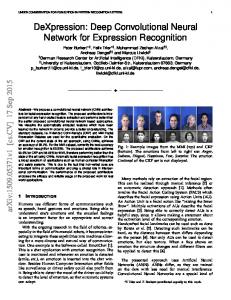
We construct 4 different CNNs that act at different resolutions. The size of the images at full resolution is 80 × 80. This size is successively divided by a factor √ √ 2 √ 3 2, 2 and 2 along each dimension giving images of size 56 × 56, 40 × 40 and 28 × 28 respectively. The constructed CNNs, named CNN80 , CNN56 , CNN40 and CNN28 , are built in a similar way. They differ essentially from the size of their respective retinas and convolution masks. The detailed architecture of the full resolution CNN is shown in Figure 2. The architectures of the other CNNs are summarized in Table 1.
Input 80x80
C1:6@74x74
Convolution 7x7
P2:6@37x37
C3:16@32x32
Convolution 6x6
Max-pooling 2x2
P4:16@8x8
C5:16@1x1
Max-pooling Convolution 8x8 4x4
Feature extraction
F6:20
Fully connected layers
Classification
Fig. 2. Architecture of the CNN80 .
Input
F7:6
Output
80x80
56x56
40x40 Final output
28x28
Fig. 3. Overall architecture of the proposed MCNN approach.
6
Pierre Buyssens, Abderrahim Elmoataz and Olivier L´ezoray Table 1. CNNs architectures. In each cell: Top: kernel size, Bottom: map size. CNN80 Retina size 80 × 80 7×7 C1 74 × 74 2×2 P2 37 × 37 6×6 C3 32 × 32 4×4 P4 8×8 8×8 C5 1×1
3.3
CNN56 56 × 56 7×7 50 × 50 2×2 25 × 25 6×6 20 × 20 4×4 5×5 5×5 1×1
CNN40 40 × 40 5×5 36 × 36 2×2 18 × 18 5×5 14 × 14 2×2 7×7 7×7 1×1
CNN28 28 × 28 5×5 24 × 24 2×2 12 × 12 5×5 8×8 2×2 4×4 4×4 1×1
Existing state–of–the–art approaches
Classical approaches in the litterature for the classification of cells rely on the extraction of shape, photometric and texture features from cells. Shape features include surface, perimeter, compacity or stretching [11]. Photometric features include mean and standard deviation of the color according to a chosen spectrum. Integral Optical Density (IOD) is also an important feature designed to reflect specific visual criteria usually used by cytopathologists [11]. It is computed as: IOD =
X
OD(x, y) ∀x, y ∈ Cell
x,y
where OD denotes the Optical Density defined as � � I(x, y) OD(x, y) = − log I0 with I0 the mean background color value, and (x, y) belonging to the cell. Finally, texture analysis aims to extract important texture features, especially features concerning the chromatin distribution contained into the cell, which indicates a possible abnormal cell. Such analysis includes morphologic features [4], wavelet features [1], shape and photometric features computed on sub–regions [11], and hierachical texture models [12] based on textons [13]. For comparison purposes with the state–of–the–art, we implemented most of these features, and extracted them from all the cells of the database at full resolution. Some of these features are computed on the whole cell, while others are computed on parts of it. Some auxiliary images used to compute these features are shown at Figure 4. We especially compute some photometric features on images of partitions (Figures 4(c) and 4(f)) to reflect the chromatin distribution within the cell: for an abnormal mesothelial, chromatin indeed tends to concentrate near the border of the cell. Cells have then been divided into concentric
Multiscale Convolutional Neural Networks
7
rings (Figure 4(c)) or into graph-based geodesic regions (Figure 4(f)) via a Region Adjacency Graph (RAG, Figure 4(e)) computed according to a watersheded version of the cell (Figure 4(d)).
(a)
(b)
(c)
(d)
(e)
(f)
Fig. 4. (a) Extracted cell, (b) textons image, (c) concentric rings image, (d) partition image, (e) part of the computed RAG, and (f) part of the graph–based concentric partition image.
A ten–fold cross validation is then processed on these features via a SVM carefully tuned with a Gaussian kernel. The final classification error rate obtained with this method is shown in Table 2. A similar ten–fold cross validation is also processed via a simple feed–forward neural network (NN), containing 103 inputs (the size of a feature vector), 80 neurons on the hidden layer, and 6 neurons as outputs (one per class). The classification error rate are reported in Table 2. Finally, these features are also classified via a Multi–Kernel SVM (MKL) approach [14]. This classification scheme aims at simultaneously learning a kernel per feature (or group of features) and weighting them. The MKL classification error rates are also reported in Table 2. 3.4
Classification results
Prior to the training of the CNNs, the images are preprocessed (First row at Figure 5). Since the complementary color of the pink colored cells is green, only this channel is kept. Pixel values are then normalized such that they lie in the range [−1, 1] (background pixel values are then close to 0). Images are then resized to fit the CNNs retina sizes. A ten–fold cross validation is processed to test the MCNN. Since the classification has to be rotation invariant, the training set is augmented with rotated images with a angle step of 10 degrees (second row at Figure 5). The training sets are then composed of about 39000 images. Initial weights of the networks
8
Pierre Buyssens, Abderrahim Elmoataz and Olivier L´ezoray
(a)
(e)
(b)
(f)
(c)
(g)
(d)
(h)
(i)
Fig. 5. First row: An abnormal mesothelial at increasing resolution. Second row: artificial rotations of a cell.
are initialized at random with small values, and we apply a stochastic learning with an annealing learning step and second order methods to speed up the training. Training ends when the error on a small subset of the training set does not decrease anymore (usually after 50 epochs). Classification results for each CNN are shown in Table 2. The error rates for the CNNs decrase while the resolution of the inputs increase since they are able to capture more information. We tested also two merging scheme of the outputs of the CNNs: – The simplest one (MCNN in Table 2) averages the outputs of each CNN; – A weighted fusion scheme (w MCNN in Table 2). For this last scheme, the weights are computed for each CNN as: w(CN Nx ) =
mean(crx ) std(crx )
where crx is the classification rate of the CNNx . This weighting gives a low weight to a CNN which has a low classification rate and/or a big standard deviation of its results. The weights indeed increases with the resolution giving more saliency to the highest resolution. A majority voting scheme (MV) has also been tested and error rate is reported in Table 2. The best combination is found without considering results of CNN28 . The lowest error rate has finally been found with the second weighting scheme (see above) without considering the results of CNN28 . The fusion of CNNs outputs (with or without CNN28 ) gives an error rate that is lower or equal to the state–of–the–art considered approaches. Table 3 shows the confusion matrix for the best approach (w MCNN /w CNN28 ). One can see that misclassified cells are mainly confused with their surrounding classes (non zeros values of the confusion matrix close to its diagonal). The good classification rate of the abnormal mesothelials (class C1 ),
Multiscale Convolutional Neural Networks
9
Table 2. Evaluation of the different methods (Standard deviation in parenthesis). Method CNN28 CNN40 CNN56 NN SVM CNN80 MV /w CNN28 MKL MCNN w MCNN w MCNN /w CNN28
Error rate 9.04% (1.07) 8.02% (1.02) 8.01% (0.98) 7.85% (0.98) 7.75% (0.95) 7.55% (0.89) 6.13% (0.84) 6.12% (0.83) 6.02% (0.82) 5.90% (0.80) 5.74% (0.79)
that are the most important for establishing a diagnosis of pleural cancer, are encouraging. The worst classification rate is for the normal mesothelials (class C3 ). Misclassified examples are mainly detected as dystrophic mesothelials (C2 ) or macrophages (C4 ). Differences between these three classes may indeed be very mild, see Figure 6 for some examples of such difficult cases.
4
Discussion
This approach avoid the design and/or the extraction of handcrafted features. Classical approaches are typically confronted to difficult tasks such as: – The design of robust and easy–to–compute features, – The evaluation of these features for their class separability capacities, – and the more general problem of features selection. Our Convolutional Neural Network approach bypasses these issues by avoiding the step related to the features. Table 3. Confusion matrix of the classification (in percentage) for the best method. In row: real class, in column: found class.
C1 C2 C3 C4 C5 C6
C1 97.41 2.39 1.24 0.14 0 0
C2 0.90 93.75 12.58 0 0 0
C3 0.77 3.85 80.22 2.56 0 0
C4 0.90 0 5.94 97.15 0.42 0.28
C5 C6 0 0 0 0 0 0 0.14 0 99.14 0.42 1.82 97.89
10
Pierre Buyssens, Abderrahim Elmoataz and Olivier L´ezoray
The approach of a committee of Convolutional Neural Networks has already been studied in [9]. The basic idea is to have multiple CNN that learn different features from the same dataset. To ensure such a learning, authors of [9] applied different distorsions to the training set for each CNN. We cannot use this approach in this work, since applying distorsions to cells may change their size or their chromatin distribution, which is not acceptable for the classification. A simple way to have more information from a simple cell is then to apply some multiresolution transformations and to build CNNs accordingly. A not–so–easy problem is also the need of a robust segmentation tool, since handcrafted features are mostly computed on a masked version of the cell. For example, if a cell is poorly segmented and its mask contains some pixels belonging to the background, the computed surface will be higher. In this case, a simple normal mesothelial could be confused with a dystrophic mesothelial or worse with an abnormal mesothelial. The segmentation has also to be fast since a virtual slide at full resolution can contain hundreds of thousands cells. For the purposes of this work, a relatively small number of cells have been manually segmented by a cytopathologist. A further work will be to extend this MCNN approach to cells that have not been segmented so as to avoid the segmentation step and replace it by a simpler cell detection module.
Abnormal Abnormal Dystrophic Dystrophic Abnormal Mesothelial Mesothelial Mesothelial Mesothelial Mesothelial Mesothelial Mesothelial
Dystrophic Macrophage Normal Normal Macrophage Dystrophic Mesothelial Mesothelial Mesothelial Mesothelial
Fig. 6. In columns, some visually similar cells belonging to different classes. Class name below each cell.
5
Conclusion
This paper presents a Multiscale Convolutional Neural Networks (MCNN) approach for a vision–based classification of cells. Relying on several CNNs acting at different resolution that do not need any handcrafted features, the proposed
Multiscale Convolutional Neural Networks
11
architecture achieves better classification rates than classical state–of–the–art approaches. Further work will involve a vision–based cell detection module in order to avoid the segmentation step. Moreover, an implemenation of MCNN on a Graphics Processing Unit (GPU) will fasten the whole process in order to approach a real–time diagnosis.
References 1. Malek, J., Sebri, A., Mabrouk, S., Torki, K., Tourki, R.: Automated breast cancer diagnosis based on gvf-snake segmentation, wavelet features extraction and fuzzy classification. J. Signal Process. Syst. 55 (2009) 49–66 2. Puls, J.H., Dytch, H.E., Roman, M.R.: Automated screening for cervical cancer using image processing techniques. In: Proceedings of 1980 FPS Users Group Meeting. (1980) 3. Churg, A., Cagle, P.T., Roggli, V.L.: Tumors of the Serosal Membrane. AFIP Atlas of Tumor Pathology – Series 4, American Registry of Pathology (2006) 4. Zarzycki, M., Schneider, T.E., Meyer-Ebrecht, D., B¨ ocking, A.: Classification of cell types in feulgen stained cytologic specimens using morphologic features. In: Bildverarbeitung f¨ ur die Medizin. (2005) 410–414 5. Nebauer, C.: Evaluation of convolutional neural networks for visual recognition. IEEE Transactions on Neural Networks 9 (1998) 685–696 6. LeCun, Y., Bottou, L., Bengio, Y., Haffner, P.: Gradient-based learning applied to document recognition. Proceedings of IEEE 86 (1998) 2278–2324 7. Hubel, D.H., Wiesel, T.: Receptive fields, binocular interaction and functional architecture in the cat’s visual cortex. Physiol 160 (1962) 106–154 8. Scherer, D., M¨ uller, A., Behnke, S.: Evaluation of pooling operations in convolutional architectures for object recognition. In: ICANN. (2010) 92–101 9. Meier, U., Ciresan, D.C., Gambardella, L.M., Schmidhuber, J.: Better digit recognition with a committee of simple neural nets. In: ICDAR, IEEE (2011) 1250–1254 10. Ueda, N.: Optimal linear combination of neural networks for improving classification performance. PAMI 22 (2000) 207–215 11. Rodenacker, K.: A feature set for cytometry on digitized microscopic images. Cell. Pathol 25 (2001) 1–36 12. Wolf, G., Beil, M., Guski, H.: Chromatin structure analysis based on a hierarchic texture model. Analytical and quantitative cytology and histology 17 (1995) 25–34 13. Julesz, B.: Textons, the elements of texture perception, and their interactions. Nature 290 (1981) 91–97 14. Rakotomamonjy, A., Bach, F., Canu, S., Grandvalet, Y.: SimpleMKL (2008)