Samuels [42] in 1959. ...... [51] D. Whitley and T. Starkweather, âGENITOR II: A distributed genetic algorithm,â J. Experimental Theoretical Artificial. Intelligence ...
1
Cooperative coevolutionary methods Nicol´as Garc´ıa-Pedrajas, C´esar Herv´as-Mart´ınez, and Domingo Ortiz-Boyer Abstract This chapter presents Covnet a cooperative coevolutionary model for evolving artificial neural networks. This model is based on the idea of coevolving subnetworks that must cooperate to form a solution for a specific problem, instead of evolving complete networks. The combination of this subnetworks is part of a coevolutionary process. The best combinations of subnetworks must be evolved together with the coevolution of the subnetworks. Several subpopulations of subnetworks coevolve cooperatively and genetically isolated. The individual of every subpopulation are combined to form whole networks. This is a different approach from most current models of evolutionary neural networks which try to develop whole networks. Covnet places as few restrictions as possible over the network structure, allowing the model to reach a wide variety of architectures during the evolution and to be easily extensible to other kind of neural networks. The performance of the model in solving three real problems of classification is compared with a modular network, the adaptive mixture of experts, and with the results presented in the literature. Covnet has shown better generalization and produced smaller networks than the adaptive mixture of experts, and has also achieved results, at least, comparable with the results in the literature. Keywords Neural networks automatic design, cooperative coevolution, evolutionary computation, genetic algorithms, evolutionary programming.
I. Introduction In the area of neural networks [1] design one of the main problems is finding suitable architectures for solving specific problems. The election of such architecture is very important, as a network smaller than needed would be unable to learn and a network larger than needed would end in over-training. The problem of finding a suitable architecture and the corresponding weights of the network is a very complex task (for a very interesting review of the matter the reader can consult [2]). Modular systems are often used in machine learning as an approach for solving these complex problems. Moreover, in spite of the fact that small networks are preferred because they usually lead to better performance, the error surfaces of such networks are more rugged and have few good solutions [3]. In addition, there is much neuropsychological evidence showing that the brain of humans and other animals consists of modules, which are subdivisions in identifiable parts, each one with its own purpose and function [4]. The objective of this chapter is showing how Cooperative Coevolution, a recent paradigm within the field of Evolutionary Computation, can be used to design of such modular neural networks. Evolutionary computation [5] [6] is a set of global optimization techniques that have been widely used in late years for training and automatically designing neural networks (see Section III). Some efforts have been made in designing modular [7] neural networks with these techniques(e.g. [8]), but in almost all of them the design of the networks is helped by methods outside evolutionary computation, or the application area for those models is limited to very specific architectures. This chapter is organised as follows: Section II explains the paradigm of cooperative coevolution; Section III shows an application of cooperative coevolution to automatic neural network design; Section IV describes the experiments carried out; and finally Section V states the conclusions of this chapter. II. Cooperative coevolution Cooperative coevolution [9] is a recent paradigm in the area of evolutionary computation focused on the evolution of coadapted subcomponents without external interaction. In cooperative coevolution a number of species are evolved together. The cooperation among the individuals is encouraged by rewarding the individuals based on how well they cooperate to solve a target problem. The work on this paradigm has shown The authors are with the Department of Computing and Numerical Analysis of the University of C´ ordoba. e-mail: {npedrajas, chervas, dortiz}@uco.es
2
that cooperative coevolutionary models present many interesting features, such as specialization through genetic isolation, generalization and efficiency [10]. Cooperative coevolution approaches the design of modular systems in a natural way, as the modularity is part of the model. Other models need some a priori knowledge to decompose the problem by hand. In many cases, either this knowledge is not available or it is not clear how to decompose the problem. This chapter describes a cooperative coevolutionary model called Covnet [11]. This model develops subnetworks instead of whole networks. These modules are combined forming ensembles that constitute a network. As M. A. Potter and K. A. De Jong [10] have stated, “to apply evolutionary algorithms effectively to increasingly complex problems explicit notions of modularity must be introduced to provide reasonable opportunities for solutions to evolve in the form of interacting coadapted subcomponents”. The most distinctive feature of Covnet is the coevolution of modules without the intervention of any agent external to the evolutionary process and without an external mechanism for combining subnetworks. Also, the use of an evolutionary algorithm for the evolution of both the weights and the architecture allows the model to be applied to tasks where there is no error function that could be defined (e.g.: game playing [12] or control [13]) in order to apply an algorithm based on the minimisation of that error, like the backpropagation learning rule, or the derivatives of that error function cannot be obtained. The most important contribution of Covnet are the following. First, it forms modular artificial neural networks using cooperative coevolution. Every module must learn how to combine with the other modules of the evolved network to be useful. Introducing the combination of nodules into the evolutionary process enforces the cooperation among the modules, as independently evolved modules are less likely to combine well after the evolutionary process have finished. Second, it develops a method for measuring the fitness of cooperative subcomponents in a coevolutionary model. This method, based on three different criteria, could be applied to other cooperative coevolutionary models not related to the evolution of neural networks. The current methods are based, almost exclusively, on measuring the fitness of the networks where the module appears. Third, it introduces a new hybrid evolutionary programming algorithm that puts very few restrictions in the subnetworks evolved. This algorithm produces very compact subnetworks, and even the evolved subnetworks alone achieved very good performance in the test problems, as it will be shown in the experimental section. III. Automatic design of artificial neural networks by means of cooperative coevolution The automatic design of artificial neural networks has two different approaches: parametric learning and structural learning. In structural learning, both architecture and parametric information must be learned through the process of training. Basically, we can consider three models of structural learning: Constructive algorithms, destructive algorithms, and evolutionary computation. Constructive algorithms [14] [15] [16] start with a small network (usually a single neuron). This network is trained until it is unable to continue learning, then new components are added to the network. This process is repeated until a satisfactory solution is found. These methods are usually trapped in local minima [17] and tend to produce large networks. Destructive methods, also known as pruning algorithms [18], start with a big network, that is able to learn but usually ends in over-fitting, and try to remove the connections and nodes that are not useful. A major problem with pruning methods is measuring the relevance of the structural components of the network in order to decide whether a connection or node must be removed. Both methods, constructive and destructive, limit the number of available architectures, thus introducing constraints in the search space of possible structures that may not be suitable to the problem. Although these methods have been proved useful in simulated data [19] [20], their application to real problems has been rather unsuccessful [21] [22] [23]. Evolutionary computation has been widely used to evolve neural network architectures and weights. There have been many applications for parametric learning [24] and for both parametric and structural learning [25] [17] [26] [27] [28] [29] [8] [30]. These works fall in two broad categories of evolutionary computation: genetic algorithms and evolutionary programming. Genetic algorithms are based on a representation independent of the problem, usually the representation is a string of binary, integer or real numbers. This representation (the genotype) codifies a network (the
3
phenotype). This is a dual representation scheme. The ability to create better solutions in a genetic algorithm relies mainly on the operation of crossover. This operator forms offspring by recombining representational components from two members of the population. The benefits of crossover come from the ability of forming connected substrings of the representation that correspond to above-average solutions [5]. This substrings are called building blocks. Crossover is not effective in environments where the fitness of an individual of the population is not correlated with the expected ability of its representational components [31]. Such environments are called deceptive [32]. Deception is a very important feature in most representations of neural networks, so crossover is usually be avoided in evolutionary neural networks [17]. One of the most important forms of deception arises from the many-to-one mapping from genotypes in the representation space to phenotypes in the evaluation space. The existence of networks functionally equivalent and with different encodings makes the evolution inefficient, and it is unclear whether crossover would produce more fitted individuals from two members of the population. This problem is usually termed as the permutation problem [33] [34] or the competing conventions problem [35]. Evolutionary programming [36] is, for many authors, the most suited paradigm of evolutionary computation for evolving artificial neural networks [17]. Evolutionary programming uses a representation natural for the problem. Once the representation scheme has been chosen, mutation operators specific to the representation scheme are defined. Evolutionary programming offers a major advantage over genetic algorithms when evolving artificial neural networks, the representation scheme allows manipulating networks directly, avoiding the problems associated with a dual representation. The use of evolutionary learning for designing neural networks dates from no more than two decades (see [2] or [35] for reviews). However, a lot of work has been made in these two decades, with many different approaches and working models, for instance, [25], [37], or [8]. Evolutionary computation has been used for learning connection weights and for learning both architecture and connection weights. The main advantage of evolutionary computation is that it performs a global exploration of the search space avoiding to become trapped in local minima as usually happens with local search procedures. G. F. Miller et al. [38] proposed that evolutionary computation is a very good candidate to be used to search the space of topologies because the fitness function associated with that space is complex, noisy, non-differentiable, multi-modal and deceptive. Almost all the current models try to develop a global architecture, which is a very complex problem. Although, some attempts have been made in developing modular networks [39] [40], in most cases the modules are combined only after the evolutionary process has finished and not following a cooperative coevolutionary model. Few authors have devoted their attention to the cooperative coevolution of subnetworks. Some authors have termed this kind of cooperative evolution (where the individuals must cooperate to achieve a good performance) symbiotic evolution [41]. More formally, we should speak of mutualism, that is, the cooperation of two individuals from different species that benefits both organisms. R. Smalz and M. Conrad [26] developed a cooperative model where there are two populations: a population of nodes, divided into clusters, and a population of networks that are combinations of neurons, one from each cluster. Both populations are evolved separately. B. A. Whitehead and T. D. Choate [29] developed a cooperative-competitive genetic model for Radial-Basis Function (RBF) neural networks. In this work there is a population of genetically encoded neurons that evolves both the centers and the widths of the radial basis functions. There is just one network that is formed by the whole population of RBF’s. The major problem, as in our approach, is to assign the fitness to each node of the population, as the only performance measure available is for the whole network. This is well known as the “credit apportionment problem”1 [26] [9]. The credit assignment used by Whitehead and Choate is restricted to RBF-like networks and very difficult to adapt to other kind of networks. D. W. Opitz and J. W. Shavlik [43] developed a model called ADDEMUP (Accurate anD Diverse Ensemble Maker giving United Predictions). They evolved a population of networks by means of a genetic algorithm 1
This problem can be traced back to the earliest attempts to apply machine learning to playing the game of checkers by Arthur Samuels [42] in 1959.
4
and combined the networks in an ensemble with a linear combination. The competition among the networks is encouraged with a diversity term added to the fitness of each network. D. E. Moriarty and R. Miikkulainen [30] [41] developed an actual cooperative model, called SANE, that had some common points with R. Smalz and M. Conrad [26]. In this work they propose two populations: one of nodes and another of networks that are combinations of the individuals from the population of nodes. Zhao et al. [44] proposed a framework for cooperative coevolution, and applied that framework to the evolution of RBF networks. Nevertheless, their work, more than a finished model, is an open proposal that aims at the definition of the problems to be solved in a cooperative environment. S-B. Cho and K. Shimohara [4] developed a modular neural network evolved by means of genetic programming. Each network is a complex structure formed by different modules which are codified by a tree structure. X. Yao and Y. Liu [45] use the final population of networks developed using the EPNet [8] model to form ensembles of neural networks. The combination of these networks produced better results than any isolated network. Nevertheless, the cooperation among the networks takes place only after the evolutionary process has finished. So, the model is neither cooperative nor coevolutionary. A. Covnet: A Cooperative coevolutionary model Covnet is a cooperative coevolutionary model, that is, several species are coevolved together. Each species is a subnetwork that constitutes a partial solution of a problem; the combination of several individuals from different species constitutes the network that must be applied to the specific problem. The population of subnetworks, that are called nodules, is made up by several subpopulations2 that evolve independently. Each one of these subpopulations constitutes a species. The combination of individuals from these different subpopulations that coevolve together is the key factor of our model. The evolution of coadapted subcomponents must address four major issues: problem decomposition, interdependence among subcomponents, credit assignment and maintenance of diversity. Cooperative coevolution gives a framework where these issues could be faced in a natural way. The problem decomposition is intrinsic in the model. Each population will evolve different species that must cooperate in order to be rewarded with high fitness values. There is no need to any a priori knowledge to decompose the problem by hand. The interdependence among the subcomponents comes from the fact that the fitness of each individual depends on how well the individual works together with the members of other species. A nodule is made up of a variable number of nodes with free interconnection among them (see Figure 1), that is, each node could have connections from input nodes, from other nodes of the nodule, and to output nodes. More formally a nodule could be defined as follows: Definition 1: (Nodule) A nodule is a subnetwork formed by: a set of nodes with free interconnection among them, the connection of these nodes from the input and the connections of the nodes to the output. It cannot have connections with any node belonging to another nodule. The input and output layers of the nodules are common, they are the input and output layers of the network. It is important to note that the genotype of the nodule has a one-to-one mapping to the phenotype, as the many-to-one mapping between them is one of the main sources of deception and the permutation problem [17]. In the same way we define a network as a combination of nodules. The definition more formally is as follows: Definition 2: (Network) A network is the combination of a finite number of nodules. The output of the network is the sum of the outputs of all the nodules that constitute the network. In practice all the networks of a population must have the same number of nodules, and this number, N , is fixed along the evolution. Some parameters of the nodule are given by the problem and for that reason they are common to all the nodules: 2 Each subpopulation evolves independently, so we can talk of subpopulations or species indistinctly, as each subpopulation will constitute a different species.
5
Fig. 1. Model of a nodule. As a node has only connections to some nodes of the nodule, the connections that are missing are represented with dashed lines. The nodule is composed by the hidden nodes and the connections of these nodes from the input and to the output.
Number of inputs Number of outputs Input vector Transfer function of the output layer these parameters are fixed for all nodules. The rest of the parameters depend on each nodule: h Number of (hidden) nodes of the nodule f i Transfer function of node i pi Partial output of node i (see explanation below) yi Output of the node i wi Weight vector of node i As the node has a variable number of connections we have considered, for simplicity, that the connections that are not present in the node have weight 0, so we can use a weight vector of fixed length for all nodes. A node could have connections from input nodes, from other nodes and to output nodes. The weight vector is ordered as follows: n m x = (1, x1 , . . . , xn ) f output
bias
input
hidden
}| { z }| { z}|{ z wi = (wi,0 , wi,1 , . . . , wi,n , wi,n+1 , . . . , wi,n+h , output
z }| { wi,n+h+1 , . . . , wi,n+h+m )
(1)
As there is no restriction in the connectivity of the nodule the transmission of the impulse along the
6
connections must be defined in a way that avoids recurrence as the aim of these work is the cooperative coevolution of feed-forward neural networks. The transmission has been defined in three steps: Step 1. Each node generates its output as a function of only the inputs of the nodule (that is, the inputs of the whole network): n X wi,j xj , pi = f i (2) j=0
this value is called partial output. Step 2. These partial outputs are propagated along the connections. Then, each node generates its output as a function of all its inputs: h n X X wi,n+j pj . wi,j xj + (3) yi = f i j=1
j=0
Step 3. Finally, the output layer of the nodule generates its output: ! h X output wi,n+h+j yi . oj = f
(4)
i=1
These three steps are repeated over all the nodules. The actual output vector of the network is the sum of the output vectors generated by each nodule. Defined in this way a nodule is equivalent to a subnetwork of two hidden layers with the same number of nodes in both layers. This equivalent model is shown on Figure 2. So, the nodule of Figure 1 could be seen as the genotype of a nodule whose phenotype is the subnetwork shown on Figure 2. This difference is important, as the model of Figure 1 considered as a phenotype would be a recurrent network. In this representation, the mapping from genotype to phenotype is one-to-one, so the deception problem above mentioned does not appear.
Fig. 2. Equivalent model with two hidden layers. Every connection from an input node represents two connections, as the input value is used in two steps (see Equations 2 and 3). Every connection from another node of the nodule represents a connection between the first and second hidden layer (see Equation 3).
7
As the nodules must coevolve to develop different behaviors we have Ns independent subpopulations of nodules3 that evolve separately. The network will always have Ns nodules, each one from one different subpopulation of nodules. Our task is not only developing cooperative nodules but also obtaining the best combinations. For that reason we have also a population of networks. This population keeps track of the best combinations of nodules and evolves as the population of nodules evolves. The whole evolutionary process is shown in Figure 3. Species creation is implicit, the subpopulations must coevolve complementary behaviors in order to get useful networks, as the combination of several nodules with the same behavior when they receive the same inputs would not produce networks with a good fitness value. So, there is no need to introduce a mechanism for enforcing diversity that can bias the evolutionary process. In the next two sections we will explain in depth the two populations and their evolutionary process. A.1 Nodule population The nodule population is formed by Ns subpopulations. Each subpopulation consists of a fixed number of nodules codified directly as subnetworks, that is, we evolve the genotype of Figure 1 that is a one-toone mapping to the phenotype of Figure 2. The population is subject to the operations of replication and mutation. Crossover is not used due to its disadvantages in evolving artificial neural networks [17]. With these features the algorithm falls in the class of evolutionary programming [36]. There is no limitation in the structure of the nodule or in the connections among the nodes. There are only one restriction to avoid unnecessary complexity in the resulting nodules, there can be no connections to an input node or from an output node. The algorithm for the generation of a new nodule subpopulation is similar to other models proposed in the literature, such as GNARL [17], EPNet [8], or the genetic algorithm developed by G. Bebis et al. [37] The steps for generating the subpopulations are the following: • The nodules of the initial subpopulation are created randomly. The number of nodes of the nodule, h, is obtained from a uniform distribution: 0 ≤ h ≤ hmax . Each node is created with a number of connections, c, taken from a uniform distribution: 0 ≤ c ≤ cmax . The initial value of the weights is uniformly distributed in the interval [wmin , wmax ]. • The new subpopulation is generated replicating the best P % of the former population. The remaining (100 − P )% is removed and replaced by mutated copies of the best P %. An individual of the best P % is selected by roulette selection and mutated. This mutated copy substitutes one of the worst (100 − P )% individuals. • There are two types of mutation: parametric and structural. The severity of the mutation is determined by the relative fitness, Fr , of the nodule. Given a nodule ν its relative fitness is defined as: Fr = e−αF (ν) .
(5)
where F (ν) is the fitness value of nodule ν. Parametric mutation consists of a local search algorithm in the space of weights, a simulated annealing algorithm [46]. This algorithm performs random steps in the space of weights. Each random step affects all the weights of the nodule. For every weight, wij , of the nodule the following operation is carried out: wij = wij + ∆wij ,
∀wij ∈ ν,
(6)
where ∆wij ∈ N (0, βFr (ν)).
(7)
where β is a positive value that must be set by the user in order to avoid large steps in the space of weights. The value of β used in all our experiments has been β = 0.75, anyway Covnet is quite robust regarding this parameter. 3
In order to maintain a coherent nomenclature we talk of one population of networks and another population of nodules. The population of nodules is divided into Ns genetically isolated subpopulations that coevolve together.
8
Fig. 3. Evolutionary process of both populations. The generation of a new population for both populations, networks and nodules, is shown in detail.
Then, the fitness of the nodule is recalculated and the usual simulated annealing criterion is applied. Being ∆F the difference in the fitness function before and after the random step: • If ∆F ≥ 0 the step is accepted. • If ∆F < 0 then the step is accepted with a probability P (∆F ) = e−
∆F T
,
where T is the current temperature. T starts at an initial value T0 and it is updated at every step, T (t + 1) = γT (t), 0 < γ < 1. The number of steps of the algorithm that are carried out on each parametric mutation is very low. Performing many steps is computationally very expensive. Parametric mutation is always carried out after structural mutation, as it does not modify the structure of the network.
9
Structural mutation is more complex because it implies a modification of the structure of the nodule. The behavioral link between parents and their offspring must be enforced to avoid generational gaps that produce inconsistency in the evolution. There are four different structural mutations: Addition of a node without connections, deletion of a node, addition of a connection with 0 weight, and deletion of a connection. The nodes are added with no connections to enforce the behavioral link with its parent. As many authors have stated, [8] [17], maintaining the behavioral link between parents and their offsprings is of the utmost importance to get a useful algorithm. All the above mutations are made in the mutation operation on the nodule. For each mutation there is a minimum value, ∆m , and a maximum value, ∆M . The number of elements (nodes or connections) involved in the mutation is calculated as follows: ∆ = ∆m + Fr (ν)(∆M − ∆m ).
(8)
So, before making a mutation the number of elements, ∆, is calculated, if ∆ = 0 the mutation is not actually carried out. There is no migration among the subpopulations. So, each subpopulation must develop different behaviors of their nodules, that is, different species of nodules, in order to compete with the other subpopulations for conquering its own niche and to cooperate to form networks with high fitness values. A.2 Network population The network population is formed by a fixed number of networks. Each network is the combination of one nodule of each subpopulation of nodules. So the networks are strings of integer numbers of fixed length. The value of the numbers is not significant as they are just labels of the nodules. The relationship between the two populations can be seen in Figure 4. It is important to note that, as the chromosome that represents the network is ordered, the permutation problem we have discussed cannot appear.
Fig. 4. Populations of networks and nodules. Each element of the network is a reference to, or a label of, an individual of the corresponding subpopulation of nodules. So the network is a vector where the first component refers to a nodule of subpopulation 1, the second component to a nodule of subpopulation 2, and so on.
The network population is evolved using the steady-state genetic algorithm [47] [48]. This term may lead to confusion as it has been proved that shows higher variance [49] and is a more aggressive and selective selection strategy [50] than the standard genetic algorithm. This algorithm is selected because we need a population of networks that evolves more slowly than the population of nodules, as the changes in the population of
10
networks have a major impact in the fitness of the nodules. The steady-state genetic algorithm avoids the negative effect that this drastic modification of the population of networks could have over the subpopulations of nodules. As the two populations evolve in synchronous generations, the modifications in the population of networks are less severe than the modifications in the subpopulations of modules. It has been also shown by some works in the area [51] [52] that the steady-state genetic algorithm produces better solutions and is faster than the standard genetic algorithm. In a steady-state genetic algorithm one member of the population is changed at a time. In the algorithm we have implemented the offspring generated by crossover replaces the two worst individuals of the population instead of replacing its parents. The algorithm allows adding mutation to the model, always at very low rates. Crossover is made at nodule level, using a standard two-point crossover. So the parents exchange their nodules to generate their offspring. Mutation is also carried out at nodule level. When a network is mutated one of its nodules is selected and is substituted by another nodule of the same subpopulation selected by means of a roulette algorithm. During the generation of the new nodule population some nodules of every population are removed and substituted. The removed nodules are also substituted in the networks. This substitution has two advantages: first, poor performing nodules are removed from the networks and substituted by potentially better ones; second, the new nodules have the opportunity to participate in the networks immediately after their creation. A.3 Fitness assignment The assignment of fitness to networks is straightforward. Each network is assigned a fitness in function of its performance in solving a given problem. If the model is applied to classification, the fitness of each network is the number of patterns of the training set that are correctly classified; if it is applied to regression, the fitness is the sum of squared errors, and so on. Assigning fitness to the nodules is a much more complex problem. In fact, the assignment of fitness to the individuals that form a solution in cooperative evolution is one of its key topics. The performance of the model highly depends on that assignment. A discussion of the matter can be found in the Introduction of [9]. A credit assignment must fulfill the following requirements to be useful: • It must enforce competition among the subpopulations to avoid two subpopulations developing similar responses to the same features of the data. • It must enforce cooperation. The different subpopulations must develop complementary features that together could solve the problem. • It must measure the contribution of a nodule to the fitness of the network, and not only the performance of the networks where the nodule is present. A nodule in a good network must not get a high fitness if its contribution to the performance of the network is not significant. Likewise, a nodule in a poor performing network must not be penalized if its contribution to the fitness of the network is positive. Otherwise, a good nodule that is temporarily assigned to poor rated networks could be lost in the evolution of the subpopulations of nodules. Some methods for calculating the fitness of the nodules have been tried. The best one consists of the weighted sum of three different criteria. These criteria, for obtaining the fitness of a nodule ν in a subpopulation π, are: Substitution (σ) k networks are selected using an elitist method, that is, the best k networks of the population. In these networks the nodule of subpopulation π is substituted by the nodule ν. The fitness of the network with the nodule of the population π substituted by ν is measured. The fitness assigned to the nodule is the averaged difference in the fitness of the networks with the original nodule and with the nodule substituted by ν. This criterion enforces competition among nodules of the same subpopulation, as it tests if a nodule could achieve better performance than the rest of the nodules of its subpopulation. The interdependencies among nodules could be a major drawback in the substitution criterion, but it does not mean that this criterion is useless. In any case, the criterion has two important features: – It encourages the nodules to compete within the subpopulations, rewarding the nodules most compatible with the nodules of the rest of the subpopulation. This is true even for a distributed representation, because
11
it has been shown that such representation is also modular. Moreover, as the nodules have no connection among them, they are more independent than in a standard network. – As many of the nodules are competing with their parents, this criterion allows to measure if an offspring is able to improve the performance of its parent. In addition, the neuropsychological evidence showing that certain parts of the brain consist of modules, that we discussed above, would support this objective. Difference(δ) The nodule is removed from all the networks where it is present. The fitness is measured as the difference in performance of these networks. This criterion enforces competition among subpopulations of nodules preventing more than one subpopulation from developing the same behavior. If two subpopulations evolve in the same way, the value of this criterion in the fitness of their nodules will be near 0 and the subpopulations will be penalized. Best k (βk ) The fitness is the mean of the fitness values of the best k networks where the nodule ν is present. Only the best k are selected because the importance of the worst networks of the population must not be significant. This criterion rewards the nodules in the best networks, and does not penalize a good nodule if it is in some poor performing networks. Considered independently none of these criteria is able to fulfill the three desired features above mentioned. Nevertheless, when the weighted sum of all of them is used they have proved to give a good performance in the problems used as tests. Typical values of the weights of the components of the fitness used in our experiment are (λδ ≃ 2λσ ≃ 60λβn ). The values of these coefficients must not only weight the importance of each criteria but also correct the differences in range of them. In order to encourage small nodules we have included a regularization term in the fitness of the nodule. Being nn the number of nodes of the nodule and nc the number of connections, the effective fitness4 , fi′ , of the nodule is calculated following: fi′ = fi − ρn nn − ρc nc .
(9)
The values of the coefficients must be in the interval 0 < ρn , ρc