Computational Intelligence and Bioinformatics Researh Group
Technical Report October
A cooperative coevolutionary algorithm for instance selection for instance-based learning Nicol´ as Garc´ıa-Pedrajas
[email protected]
Juan A. Romero del Castillo
[email protected]
Domingo Ortiz-Boyer
[email protected]
Computational Intelligence and Bioinformatics Research Group University of C´ ordoba Spain (http://cib.uco.es/)
Abstract This paper presents a cooperative evolutionary approach for the problem of instance selection for instance based learning. The presented model takes advantage of one of the most recent paradigms in the field of evolutionary computation: cooperative coevolution. This paradigm is based on an approach similar to the philosophy of divide and conquer. In our method, the set of instances is divided into several subsets that are searched independently. A population of global solutions relates the search in the different subsets and keeps track of the best combinations obtained. The proposed model has the advantage over standard methods that it does not rely on any specific distance metric or classifier algorithm. Most standard methods are specifically designed to k-NN classifiers, however our proposal can be used with any classifier and may benefit from any specific bias of that classifier. Additionally, the fitness function of the individuals considers both storage requirements and classification accuracy, and the user can balance both objectives depending on his/her specific needs, assigning different weights to each one of these two terms. The proposed model is favourably compared with some of the most successful standard algorithms, namely IB3, ICF and DROP3, and with a genetic algorithm using the CHC philosophy. The comparison shows a large advantage of the proposed algorithm in terms of storage requirements, and is, at least, as good as any of the other methods in terms of generalisation error. A large set of 50 problems from the UCI Machine Learning Repository is used for the comparison. Additionally, a study of the effect of instance label noise is carried out, showing the robustness of the proposed algorithm. Keywords: Instance selection; Evolutionary algorithms c
2006 CIBRG.
1
CIBRG TR-01-2006
1. Introduction The overwhelming amount of data that is available nowadays in any field of research poses new problems for data mining and knowledge discovery methods. This huge amount of data makes most of the existing algorithms inapplicable to many real-world problems. Two approaches have been used to face this problem: scaling up data mining algorithms Provost and Kolluri (1999) and data reduction. Nevertheless, scaling up a certain algorithm is not always feasible. Data reduction consists of removing from the data missing, redundant, and/or erroneous data to get a tractable amount of data. Data reduction techniques use different approaches: feature selection Liu and Motoda (1998), feature-value discretisation Hussain et al. (1999), and instance selection Blum and Langley (1997). This paper deals with instance selection for instance based learning. Instance selection Liu and Motoda (2002) consists of choosing a subset of the total available data to achieve the original purpose of the data mining application as if the whole data is used. Different variants of instance selection exists. Many of the approaches are based on some form of sampling Cochran (1977) Kivinen and Mannila (1994). However, there are other methods that are based on different principles. Our aim is focused on instance selection for instance-based learning. We can distinguish two main models Cano et al. (2003): instance selection as a method for prototype selection for algorithms based on prototypes (such as k-Nearest Neighbours) and instance selection for obtaining the training set for a learning algorithm that uses this training set (such as classification trees or neural networks). Although the proposed model is used for the former approach, it can be used for the latter without any significant modification. The problem of instance selection for instance based learning can be defined as Brighton and Mellish (2002) “the isolation of the smallest set of instances that enable us to predict the class of a query instance with the same (or higher) accuracy than the original set”. It has been shown that different groups of learning algorithms need different instance selectors in order to suit their learning/search bias Brodley (1995). This may render many instance selection algorithm useless, if their philosophy of design is not suitable for the problem at hand. Our algorithm does not assume any structure of the data or any behaviour of the classifier, adapting the instance selection to the performance of the classifier. The proposed method for instance selection for instance based learning is based on cooperative coevolution. Cooperative coevolution is a recent paradigm within the field of evolutionary computation that focuses on the cooperative evolution of coadapted subcomponents Moriarty and Miikkulainen (1996). The basic idea underlying cooperative coevolution is the evolution of partial solutions to complex problems that can cooperate to make up a global solution. In this way, our model divides the problem of instance selection into different subproblems, easier to be efficiently solved. Evolutionary computation (EC) Goldberg (1989) Michalewicz (1994) is a set of global optimisation techniques that have been widely used in the last few years for almost every problem within the field of Artificial Intelligence. In evolutionary computation a population (set) of individuals (solutions to the problem faced) are codified following a code similar to the genetic code of plants and animals. This population of solutions is evolved (modified) over a certain number of generations (iterations) until the defined stop criterion is fulfilled.
2
Cooperative instance selection
Each individual is assigned a real value that measures its ability to solve the problem, which is called its fitness. In each iteration new solutions are obtained combining two or more individuals (crossover operator) or randomly modifying one individual (mutation operator). After applying these two operators a subset of individuals is selected to survive to the next generation, either by sampling the current individuals with a probability proportional to their fitness, or by selecting the best ones (elitism). The repeated processes of crossover, mutation and selection are able to obtain increasingly better solutions for many problems of Artificial Intelligence. Within the field of EC there is a paradigm that focuses on approaching complex tasks by dividing them into simpler subproblems. This paradigm is Cooperative Coevolution (CC). In CC each individual is not the solution to a problem, but just a partial solution. Different individuals must be combined to obtain a solution. In this way, modularity is an intrinsic aspect of the methodology. The proposed model is based on CC. Brighton and Mellish Brighton and Mellish (2002) argued that the structure of the classes formed by the instances can be very different, thus, an instance selection algorithm can have a good performance in a problem and be very inefficient in another problem. They state that the instance selection algorithm must gain some insight to the structure of the classes to perform an efficient instance selection. However, this insight is usually not available or very difficult to acquire, especially in real-world problems with many variables and complex boundaries between the classes. In such a situation, an approach based on EC may be of help. The approaches based on EC do not assume any special form of the space, the classes or the boundaries between the classes, they are only guided by the ability of each solution to solve the task. In this way, the algorithm learns from the data the relevant instances without imposing any constraint in the form of the classes or the boundaries between them. In a first approach our method shares some of the ideas underlying stratified random sampling Liu and Motoda (2002). In stratified random sampling a setPof N instances is divided into k nonoverlapping subsets of sizes N1 , N2 , . . . , Nk , where i Ni = N . Each subset is called a stratum. Then a random sample is extracted from each stratum. In our approach the set of instances is stratified and each stratum is assigned to evolve following a genetic algorithm. In this way, the initial populations are constructed by stratified random sampling. The evolution of the individuals in each population optimises the classification and storage requirements within the stratum. The main contribution of our method is the use of cooperative coevolution to promote collaboration among the strata. In this way, another population is created that keeps track of the best combination of individuals so far and enforces the cooperation among the individuals that evolve using instances of each stratum. The model allows the interaction among the simpler searches that are carried out in each stratum, instead of performing a large search in the whole set. This paper is organised as follows: Section 2 reviews some related work; Section 3 presents the proposed model for instance selection based on cooperative coevolution; Section 4 states the experimental setup; Section 5 shows the results of the experiments; and Section 6 states the conclusions of our work and future research lines.
3
CIBRG TR-01-2006
2. Related work Genetic algorithms have been used before for instance selection, considering this task a search problem. The application is easy and straightforward. Each individual is a binary vector that codes a certain sample of the training set. The evaluation is usually made considering both data reduction and classification accuracy. Examples of applications of genetic algorithms to instance selection can be found in Kuncheva (1995), Ishibuchi and Nakashima (2000) and Reeves and Bush (2001). One of the most interesting advantages of the application of evolutionary computation to instance selection is that evolutionary approaches do not depend on specific classifiers, and can be used with any instance based classifier. This is in contrast with most standard algorithms that are specifically designed for k-NN classifiers. For instance, Reeves and Bush Reeves and Bush (2001) used a genetic algorithm to select instances for RBF neural networks. Cano et al. Cano et al. (2003) performed a comprehensive comparison of the performance of different evolutionary algorithms for instance selection. They compared a generational genetic algorithm Goldberg (1989), a steady-state genetic algorithm Whitley (1989), a CHC genetic algorithm Eshelman (1990), and a population based incremental learning algorithm Baluja (1994). They found that evolutionary based methods were able to outperform classical algorithms in both classification accuracy and data reduction. Among the evolutionary algorithms, CHC was able to achieve the best overall performance. The major problem addressed when applying genetic algorithms to instance selection is the scaling of the algorithm. As the number of instances grows, the time needed for the genetic algorithm to reach a good solution increases exponentially, making it totally useless for large problems. Recently, Cano et al Cano et al. (2005) Cano et al. (2006) have proposed a stratified approach to alleviate this difficulty. To the best of our knowledge there is no previous application of cooperative coevolution to instance selection for instance based learning.
3. Instance selection by cooperative coevolution In cooperative coevolution a number of species are evolved together. Cooperation among individuals is encouraged by rewarding the individuals for their join effort to solve a target problem. The work in this paradigm has shown that cooperative coevolutionary models present many interesting features, such as specialisation through genetic isolation, generalisation and efficiency Potter and de Jong (2000). Cooperative coevolution approaches the design of modular systems in a natural way, as the modularity is part of the model. Other models need some a priori knowledge to decompose the problem by hand. In many cases, either this knowledge is not available or it is not clear how to decompose the problem. The cooperative coevolutionary model offers a very natural way for modelling the evolution of cooperative parts. Our model is inspired on a stratified approach. It is obvious that if we could perform independent searches within each stratum, the task would be simplified. However, this is not possible as the nearest neighbours of each instance can be in any stratum. Considering only the instances in the stratum will yield to erroneous evaluation of the neighbours. So, we
4
Cooperative instance selection
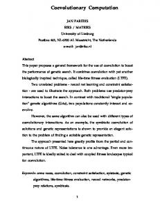
Figure 1: Distribution of the dataset among the different subpopulations of instances and representation of an individual.
develop a model that combines a search in independent stratum together with a method of combining those independent searches in such a way that the results are useful and efficient. Our cooperative model, called Cooperative Coevolutionary Instance Selection (CCIS) algorithm, is based on two separate populations that evolve cooperatively.1 These two populations are: • Population of selectors. This population is made up of Ns independent subpopulations. The whole training set is divided into Ns approximately equal parts and each part is assigned to a subpopulation. Each individual of a subpopulation is a subset of instances for the corresponding subset of training instances (see Figure 1). Every subpopulation is evolved using a standard genetic algorithm. The individuals of these subpopulations will be called throughout the paper selectors. We will use the term population of selectors when referring to all the subpopulations of selectors as a whole. • Population of combinations of instances sets. Each member of the population of combinations is the combination of an individual from every subpopulation. The population of combinations keeps track of the best combinations of selectors for different subsets of instances, selecting the combinations that are promising for the final global selector selection of the whole dataset. The individuals of this population will be called throughout the paper combinations. The individuals of the populations of selectors are subject to two operations: crossover and mutation. The crossover operator is the Half Uniform Crossover (HUX) Eshelman (1990). This operator generates two offspring from two parents. Each offspring inherits 1. A model sharing some of these basic ideas has already been successfully applied to the evolution of modular neural networks Garc´ıa-Pedrajas et al. (2002) and ensembles of neural networks Garc´ıa-Pedrajas et al. (2005).
5
CIBRG TR-01-2006
Figure 2: Populations of selectors and combinations. Each element of the population of combinations is a reference to an individual of the corresponding subpopulation of selectors.
the matching bits of the two parents, and half of the non-matching bits from each parent alternately. Mutation operator takes two forms: random mutation and local search mutation. Random mutation randomly modifies some of the bits of an individual. Local search mutation performs a local search algorithm to help the genetic algorithm to fine tune a good solution.2 The local search algorithm is a Reduced Nearest Neighbour Gates (1972) algorithm considering only the patterns in the stratum assigned to the subpopulation. This algorithm is fast enough and greatly improves the performance of CCIS. The two populations evolve cooperatively. Each generation of the whole system consists of N generations of the combination population followed by M generations of the selector population. The relationship between the two populations can be seen in Figure 2. The second basis of our model is the use of multiple criteria in the evaluation of the fitness of the individuals of the population of selectors and combinations. The evaluation of several objectives for each selector allows the model to encourage cooperation, rewarding the selectors not only for their performance in solving the given problem, but also for other aspects, such as whether they are different from other selectors, whether they are useful in the combinations or anything else considered relevant by the designer. Each individual in the population of selectors is evaluated combining three different criteria. Each criterion is intended to evaluate the individual in a different aspect. We must note that the fitness of the selectors is not directly measurable within the problem framework as they constitute only a partial solution. These three criteria are:
2. The use of a local search algorithm is common in evolutionary computation as these kinds of algorithms usually find it difficult to converge to an optimal solution.
6
Cooperative instance selection
Error. (ǫ) Training accuracy when applying a 1-NN learning rule3 using the instances selected by the individual, and only considering the instances in the subset assigned to the subpopulation. It is only an estimation of the ability of the individual as the instances of the other subpopulations are not considered. Reduction. (ρ) Percentage of reduction of the individual. It is measured as the number of instances of the individual, that the number of bits set to 1, divided by the size of the instance subset. Difference. (δ) The individual is removed from all the combinations where it is present, and the performance of such combinations with the individual removed is measured. The value of this criterion is measured as the difference in performance of these combinations with and without the individual. This criterion enforces competition among subpopulations of selectors preventing subpopulations with few useful instances to harm the storage reduction of the algorithm. If a subpopulation does not contain useful instances, the value of this criterion in the fitness of their individuals will be near 0 and only a few instances will be included in the final solution. The fitness of the individuals is measured using a weighted sum of these three criteria. In this way, the fitness of individual i, fi , is given by: fi = wǫ (1 − ǫ) + wρ ρ + wδ δ,
(1)
where wǫ , wρ , and wδ , must be fixed by the user. We chose these weights with the constraint wǫ + wρ + wδ = 1. The evaluation of the combinations is made considering two criteria: reduction of storage, ρ, and classification accuracy, ǫ, using a 1-NN learning rule. The fitness of individual j, Fj , is given by: Fj = w(1 − ǫ) + (1 − w)ρ,
(2)
where 0 ≤ w ≤ 1. The weight w is needed to avoid a negative effect that may occur due to the asymmetry of the two values of the fitness function: the reduction value can be made arbitrarily high, until the maximum value 1, by just removing more instances. To avoid this effect w must be small, so that if the reduction is too large, the accuracy will be negatively affected and the fitness of the individual penalised. The generation of a new population of combinations is made using a steady-state genetic algorithm Whitley and Kauth (1988) Whitley (1989).4 This algorithm is chosen due to the fact that we need a population of combinations that evolves more slowly than the population of selectors, as the changes in the population of combinations have a major impact on the fitness of the selectors. The steady-state genetic algorithm avoids the negative effect that this drastic modification of the population of combinations may have over the subpopulations of selectors. It has also been shown by some papers in the area Whitley 3. Modifying the classifier used in this criterion we can use our model in any learning environment, not just for a k-NN learning rule. 4. It is important to note that the specific evolution of both populations is not relevant to the success of the model. It is the cooperative coevolution of the two populations that is the key aspect of the method.
7
CIBRG TR-01-2006
and Starkweather (1990) Syswerda (1991) that the steady-state genetic algorithm produces better solutions than the standard genetic algorithm. The steady-state algorithm has three features that are different from the standard genetic algorithm: • The crossover generates just one individual. Two parents are chosen by means of a roulette selection algorithm. One of the two offspring is selected randomly. • The selected offspring replaces the worst individual of the population instead of replacing one of its parents. • Fitness is assigned to the members of the population in function of their rank and not as their absolute fitness value. The algorithm allows adding mutation to the model, always at very low rates. Usually mutation rate ranges from 1% to 5%. In our model we have modified this standard algorithm allowing the replacement of the n worst individuals instead of replacing just the worst one. In our experiments n = 2. We also selected the two offspring of the crossover operator, instead of just one. Crossover is made at selector level, using a standard two-point crossover. Thus the parents exchange their selectors to generate their offspring. Mutation is also carried out at selector level. When a combination is mutated, one of its selectors is randomly chosen and substituted by another one of the same subpopulation selected by means of a roulette algorithm. During the generation of the new selector subpopulation, some selectors of every subpopulation are removed and substituted by new ones. The removed selectors are also substituted in the combinations. This substitution has two advantages: first, poor performing selectors are removed from the combinations and substituted by potentially better ones; second, new selectors have the opportunity to participate in the combinations immediately after their creation. The complete algorithm is detailed in Algorithm 1. Mutation in the population of combinations is performed with probability Pmutation . In the subpopulations of instance sets random mutation is performed with probability Prandom . Once a selector is chosen for mutation, each bit is flipped with a probability Pbit . RNN mutation is performed with probability Prnn . The key aspect of our work is the use of two separate populations that cooperate in solving the instance selection problem. This architecture has the following advantages over other approaches: • The cooperative method approaches the problem of instance selection by means of an automatic decomposition in simpler problems. The cooperation among the individuals that solve those simple problems provides a global solution to the problem. • Unlike other approaches that are specifically designed for k-NN classifiers, our algorithm can be used with any classifier. In this way, the model can be used for any instance based classifier, such as a neural network, a tree or a support vector machine. 8
Cooperative instance selection
Algorithm 1: Cooperative coevolutionary instance selection (CCIS). Data : A training set S = {(x1 , y1 ), . . . , (xn , yn )}, a number of nearest neighbours k, and the number of iterations N, M . Result : The reduced training set: S ′ ⊂ S. 1 Initialise population of combinations 2 Initialise subpopulations of selectors while Stopping criterion not met do for N iterations do 3 Evaluate population of combinations 4 Select two individuals by roulette selection and perform two point crossover 5 Offspring substitutes two worst individuals 6 Perform mutation with probability Pmutation
7 8 9 10 11 12
end for M iterations do Evaluate subpopulations of selectors Copy Elitism% to new subpopulation Fill (1-Elitism)% by HUX crossover Apply random mutation with probability Prandom Apply RNN mutation with probability Prnn Evaluate population of combinations end end
9
CIBRG TR-01-2006
• The flexibility of the weight of classification accuracy and storage requirements in the fitness of the individuals provide a way to adjust the algorithm to the special needs of any task. Therefore, if we are interested either in a large storage reduction or in a good classification accuracy we can adjust the weights accordingly. • The proposed method can be distributed with a few modifications. Then next section shows how the distribution can be carried out. Section 5.1 shows the performance of the decoupled version of the algorithm that can be implemented in a distributed/parallel architecture. 3.1 Distributed implementation One major drawback of our proposed algorithm is that a distributed implementation is problematic due to the coupled evolution of combinations and selectors. Although the evaluation of selectors of different subpopulations can be performed separately, the need to evaluate all the combinations after each modification of the subpopulations (line 12 in Algorithm 1) prevents any efficient distributed implementation of the algorithm. Thus, the main problem with a distributed implementation is the coupling of the evolution of the M generations of the population of combinations and the N generations of the subpopulations of selectors. We propose an alternative implementation where the evaluation of the combinations is made only after the N generations of the subpopulations of selectors. The general evolution is shown in Algorithm 2. We call this implementation the decoupled version of the algorithm. The main drawback of this version is that during the inner loop (line 7 to 11) the evaluation of the selectors is only approximate, as the population of combinations is not reevaluated until line 12. Nevertheless, Section 3.1 presents results that show that this decoupled implementation is able to achieve almost as good a performance as the original one in terms of storage reduction. This version allows the distribution of the evaluation and evolution of the different subpopulations of selectors. This is the most computationally expensive part of the algorithm. Additionally, the evaluation of the combinations can be made in parallel, without any modification of the algorithm. 3.2 Evaluating instance selection algorithms The evaluation of a certain instance selection algorithm is not a trivial task. We can distinguish two basic approaches: direct and indirect evaluation Liu and Motoda (2002). Direct evaluation evaluates a certain algorithm based exclusively on the data. The objective is to measure at which extent the selected instances reflect the information present in the original data. Some proposed measures are entropy Cover and Thomas (1991), moments Smith (1998), and histograms Chaudhuri et al. (1998). Indirect methods evaluate the effect of the instance selection algorithm on the task at hand. So, if we are interested in classification we evaluate the performance of the used classifier when using the reduced set obtained after instance selection as learning set. Therefore, when evaluating instance selection algorithms for instance learning, the most usual way of evaluation is estimating the performance of the algorithms on a set of bench10
Cooperative instance selection
Algorithm 2: Decoupled cooperative coevolutionary instance selection (D–CCIS). Data : A training set S = {(x1 , y1 ), . . . , (xn , yn )}, a number of nearest neighbours k, and the number of iterations N, M . Result : The reduced training set: S ′ ⊂ S. 1 Initialise population of combinations 2 Initialise subpopulations of selectors while Stopping criterion not met do for N iterations do 3 Evaluate population of combinations 4 Select two individuals by roulette selection and perform two point crossover 5 Offspring substitutes two worst individuals 6 Perform mutation with probability Pmutation
7 8 9 10 11
12
end for M iterations do Evaluate subpopulations of selectors Copy Elitism% to new subpopulation Fill (1-Elitism)% by HUX crossover Apply random mutation with probability Prandom Apply RNN mutation with probability Prnn end Evaluate population of combinations end
11
CIBRG TR-01-2006
mark problems. In those problems several criteria can be considered, such as Wilson and Martinez (2000): storage reduction, generalisation accuracy, noise tolerance, and learning speed. Speed considerations are difficult to measure, as we are evaluating not only an algorithm but also a certain implementation, so we do not consider speed in our evaluation. We will test our algorithm and other four algorithms on several datasets and evaluate their data reduction ability and generalisation accuracy. Section 5.2 is concerned with to the study of the noise tolerance of each algorithm.
4. Experimental setup In order to make a fair comparison between the standard algorithms and our proposal we have selected a large set of 50 problems from the UCI Machine Learning Repository Hettich et al. (1998). For estimating the storage reduction and generalisation error we used a k-fold cross-validation method. In this method the available data is divided into k approximately equal subsets. Then, the method is learned k times, using in turn each one of the k subsets as testing set, and the remaining k − 1 subsets as training set. The estimated error is the average testing error of the k subsets. A fairly standard value for k is k = 10. A summary of these data sets is shown in Table 1. The table shows the generalisation error of a 1-NN classifier, that can be considered as a baseline measure of the error of each dataset. These datasets can be considered representative of problems from small to medium size. The use of t-tests Anderson (1984) for the comparison of several classification methods has been criticised in several papers Dietterich (1998). This test can provide an accurate evaluation of the probability of obtaining the observed outcomes by chance, but it has limited ability to predict relative performance even on further data set samples from the same domain, let alone on other domains. Moreover, as more data sets and classification algorithms are used, the probability of type I error, a true null hypothesis incorrectly rejected, increases dramatically. Multiple comparison tests can be used in order to circumvent this last problem, but these tests are usually not able to establish differences among the algorithms.
12
Cooperative instance selection
Table 1: Summary of data sets. The features of each data set can be C(continuous), B(binary) or N(nominal). The Inputs column shows the number of inputs, as it depends not only on the number of input variables but also on their type. Data set abalone anneal audiology autos balance breast-cancer cancer card dermatology ecoli gene german glass glass-g2 heart heart-c hepatitis horse hypothyroid ionosphere iris kr vs. kp labor led24 liver lrs lymphography new-thyroid optdigits page-blocks pendigits 1 phoneme pima post-operative primary-tumor promoters satimage segment sick sonar soybean texture tic-tac-toe vehicle vote vowel waveform wine yeast zoo
Cases 4177 898 226 205 625 286 699 690 366 336 3175 1000 214 163 270 302 155 364 3772 351 150 3196 57 200 345 531 148 215 5620 5473 10992 5404 768 90 339 106 6435 2310 3772 208 683 5500 958 846 435 990 5000 178 1484 101
Features C B 7 6 14 61 15 4 4 3 9 6 4 1 1 7 6 3 9 9 13 6 3 6 13 7 2 7 20 33 1 4 34 8 3 24 6 101 3 9 5 64 10 16 5 8 1 14 36 19 7 20 60 16 40 18 16 10 40 13 8 1 15
N 1 18 8 6 6 5 32 60 11 4 13 2 2 5 6 7 3 57 2 19 9 -
Classes
Inputs
1-NN error
29 5 24 6 3 2 2 2 6 8 3 2 6 2 2 2 2 3 4 2 3 2 2 10 2 10 4 3 10 5 10 2 2 3 22 2 6 7 2 2 19 11 2 4 2 11 3 3 10 7
10 59 93 72 4 15 9 51 34 7 120 61 9 9 13 22 19 58 29 34 4 38 29 24 6 101 38 5 64 10 16 5 8 20 23 114 36 19 33 60 82 40 9 18 16 10 40 13 8 16
0.8034 0.0157 0.3273 0.3300 0.2226 0.3714 0.0479 0.2174 0.0472 0.2060 0.2647 0.3120 0.2952 0.2000 0.2333 0.2400 0.1933 0.3667 0.0692 0.1314 0.0467 0.0828 0.0600 0.5350 0.3794 0.1887 0.1929 0.0333 0.0256 0.0362 0.0066 0.0952 0.3013 0.4889 0.6515 0.2500 0.0927 0.0355 0.0430 0.1550 0.0779 0.0105 0.0779 0.2929 0.0675 0.2919 0.2860 0.0353 0.4689 0.0600
13
CIBRG TR-01-2006
To avoid these problems we perform, in a first approach, a single significance test for every pair of algorithms. This test is a sign test on the win/draw/loss record of the two algorithms across all datasets. If the probability of obtaining the observed results by chance, the p-value of the sign test, is below 5% we conclude that the observed performance is indicative of a general underlying advantage to one of the algorithms with respect to the type of learning task used in the experiments. Nevertheless, the comparison using sign tests has two potential problems: Firstly, the differences between the two algorithms compared must be very marked for the test to find significant differences Demˇsar (2006); secondly, on some occasions the p-value of the test can be above or below the critical value due to a single modification of the outcome of one experiment, making the result of the test less reliable. So, as an additional test we have used the Wilcoxon test for comparing pairs of algorithms. This test is chosen because it was found to be the best one for comparing pairs of algorithms in a recent paper Demˇsar (2006). The formulation of the test Wilcoxon (1945) is the following: Let di be the difference between the error values of the methods on i-th dataset. These differences are ranked according to their absolute values; in case of ties an average rank is assigned. Let R+ be the sum of ranks for the datasets on which the second algorithm outperformed the first, and R− the sum of ranks where the first algorithm outperformed the second. Ranks of di = 0 are split evenly among the sums: R+ =
X
rank(di ) +
X
rank(di ) +
di >0
and, R− =
1X rank(di ), 2
(3)
di =0
di