Cooperative Multisite Production Re-scheduling Jaime Lloret1, Jose P. Garcia-Sabater2, and Juan A. Marin-Garcia3 1
Department of Communications
[email protected] 2,3 Department of Enterprise Organization Camino Vera s/n, 46022, Valencia, Spain
[email protected],
[email protected]
Abstract. One of the main issues in cooperative enterprise planning and scheduling is how to re-assign tasks without involving too many components of every enterprise and implying too many changes in the whole system. We propose a new system that is able to re-schedule tasks in cooperative multisite production automatically avoiding one of the main problems that have schedule programmers that are in charge of two or more cooperative enterprises. The system is based on making virtual groups of machines that perform the same tasks and establishes links between machines from different groups. We will describe the algorithm in detail and we will validate it using a case of study. Results show that our proposal gives better performance. Keywords: Scheduling, Cooperative decision making, Supply chain, cooperative-group-based model.
1 Introduction Customer requirements have changed drastically over the past decades: customers want lower costs, higher quality and so on [1]. In order to meet this wide range of customer requirements, and due to narrow profit margins and order-driven production, optimal and flexible operation is becoming more and more important in all areas of industry from a strategic perspective as a way to achieve a competitive advantage [1; 2]. Nowadays, most machine lines in manufacturing plants are shared resources. Hence, the same machines are used to produce different product types, with a set-up involved when production is switched from one product type to another [1]. Planning is one of the major issues in today’s competitive marketplace where all operations of the jobs resulting from customer orders must be executable in the technological sequences on the machines within the planned and contracted delivery time and all necessary tools must be available [3]. Short-term production planning is a challenging task because it poses a complex machine/job loading, sequencing and scheduling problem. Effective production planning can result in reduction of manpower, work-in-process inventory cost, and other production costs by minimizing machine idle time and increase the number of on-time job deliveries [3]. During the recent years, the performance of computers and optimization software has reached a point where it has become feasible to use dynamic Y. Luo (Ed.): CDVE 2008, LNCS 5220, pp. 156–163, 2008. © Springer-Verlag Berlin Heidelberg 2008
Cooperative Multisite Production Re-scheduling
157
information to optimize the production plans [2]. Machine loading is one of the process planning and scheduling problems that involves assigning a set of part types on a set of machines to optimize some predefined measures of productivity [3]. Several characteristics and restrictions regarding the manufacturing activities need to be scheduled [1; 4]: Some tasks need to be performed consecutively, others are disjunctive; some have to be done concurrently, and some bear simple precedence relationships. The performance of any single activity block cannot be split among multiple jobs. However, for certain activities, more than one job is (simultaneously or sequentially) needed. Each product requires a sequence of operations in a certain order. It is different for each product. Each order is defined by product, quantity, delivery time and place to deliver it. A single product can be processed by only one machine at each assembly stage, the practice of pre-empting it from one machine to get it completed on another not being viable. Each product type undergoes the assembly process in the same sequence as others, being allowed to skip one assembly stage whenever specific components are not required. The problem of the supply chain department can now be defined as follows: For given customer orders (product, quantity, due date and place) for the planning horizon, a machine loading plan must be determined which minimizes the number of delays and minimize the cost. We consider an automotive supplier group of firms. Each plant consists of several work centers, each of them with similar machines that have to meet a regular demand for different products with a limited number of stages. The aim of this research is to develop a Machine Loading Sequencing model to improve the production efficiency. The proposed production scheduling system will take into account the quality of product and service, inventory holding cost, and machine utilization. The remainder of this paper is structured as follows. Section 2 shows the related works. Section 3 describes the re-scheduling algorithm operation and the parameters needed to run. In order to validate our proposal we present a study case in section 4. Section 5 concludes the paper
2 Related Works Flexible flow lines (they are flow lines with several parallel machines on some or all production stages) can be found in a vast number of industries. They are especially common in the process industry. Numerous examples are given in the literature, including the chemical industry, electronics manufacturing and so on [5;6]. Scheduling for machining parts and planning for assembly operations have been studied independently. However, these problems should be treated simultaneously [7]. Scheduling is an important phase in short-term production planning. A scheduling procedure determines an exact production time and a machine assignment for each operation. Scheduling flexible flow lines comprises three sub-problems: Batching, loading and sequencing. Batching occurs only if setup costs or times are not negligible and several jobs of the same product type have to be produced. In this case, it might be advantageous to batch multiple jobs of the same product type and produce them with just a single setup in the beginning. A batching sub-procedure has to decide how many units to produce consecutively, i.e. to calculate the batch-sizes. Only a few
158
J. Lloret, J.P. Garcia-Sabater, and J.A. Marin-Garcia
studies explicitly consider setup times between jobs. Most studies assume that either no setup has to be performed or that setup times are sequence-independent and there is only a single unit of each product type. In this case, a job’s setup time may be added to its process time and does not have to be considered explicitly. However, if setup times are sequence-dependent or if several jobs of the same product type have to be produced, setups have to be considered explicitly. The loading sub-problem refers to the allocation of operations to machines. For each operation of a job, one of the parallel machines has to be selected. If batch-sizes have been calculated, the loading sub-problem is to assign the batches to machines. When all loading decisions have been made, the routes through the system are determined. Thus, the remaining sequencing sub-problem is essentially a job shop scheduling problem. The sequencing sub-problem is to order the jobs being assigned to a machine, i.e. to calculate a production sequence for all machines. Rescheduling, just as its name implies, means to schedule the jobs again, together with a set of new jobs. There are several references on rescheduling approaches. Most of them consider only one machine rescheduling. Wu et al. [8] consider the problem of rescheduling a job shop after a disruption to minimize the make span and the disruption from the original schedule.
3 Re-scheduling Algorithm 3.1 Parameters Definition In order to describe our proposal, first we have to give some definitions about the elements taken into account in the algorithm and define several parameters that will be used in the operation of the algorithm. A node in our proposal will be any element, machine, device or automatic machine that will be used in the schedule. A site could be a factory, a production plant, or even an area of a production plant where the nodes are placed. All the nodes in the same site are interconnected through a physical data network, so they are communicated. A virtual group (from now we will call them just “group”) is form by nodes that can be placed in the same site or in different sites, but what they have in common is that they can perform the same tasks. There could be nodes that can perform different tasks, so the can be in different groups at the same time. To simplify our explanation we will suppose that all nodes can perform only one task because it usually happens. There is a link between a pair of nodes when a piece of a first node placed in a first group will be sent to the second node placed in a second group to produce a new piece. In our explanations links have only one direction, but we could modify to be bidirectional. First, we are going to define several identifiers that will be used in the algorithm. They are shown in table 1. Each node has a unique identifier in the group and each group has a unique identifier. We define λ as the capacity parameter. Every node has its λ parameter. It is used to determine the best node in a group to assign a task. The more capacity has a node in of a group, better is the element to be chosen to do a task. It depends on the cost, the production, the product quality, the grade of saturation, the maximum links and the available links. λ parameters from different groups are not comparable, because λ
Cooperative Multisite Production Re-scheduling
159
parameter is calculated by some parameters that depend on the type of the machines, so machines from different groups give different ranges of values. The descriptions of the parameters used to calculate λ parameter are shown in table 2. Table 1. Identifiers that will be used in the algorithm Name
Description
SiteID
It is the site identifier. A site could be an enterprise or factory. The first time a node joins a site, there is a computer in the network that assigns it the SiteID, but it could be assigned manually. It is the group identifier. It is assigned manually depending on the tasks the node is able to do. There will be as much groups as processes or tasks for the production of the pieces. All groups have a unique groupID and all nodes in the same group have the same groupID. It is an identifier of a node in the site. It is unique for each node of the same group. It can be assigned manually or acquired automatically by a computer when the node joins the first time a group.
GroupID
NodeID
Table 2. Parameters taken into account for λ calculation Name
Parameter
Product FTTi Quality (First Time Through) Grade of S Saturation
Expression U − R − D − scrap FTT = U
S = 100·∑ i ,l
Cost
Ci
q C = il pi
Production
Pi
-
q i ,l pi ·d l
Description It gives the quality of the product i. It is the percentage of units that finish the production process and satisfy the quality rules when the machine starts. It gives the saturation of the node. It depends on the time of response and on the response at time. It is measured in %. It gives the cost of a product i for that node at a certain order.
It gives the capacity of a node to produce a product i. It is measured in pieces per minute. Maximum Max_Links It is the maximum number of simultaneous links incoming links that it has with nodes from other groups. Available Ava_Links It is the available number of incoming links links that it has with nodes from other groups. Note: Where U is the quantity of units entering the process is the number of pieces that enter the process, R is the number of units with defects that are repaired inside the process (reworks), D is the quantity of units that have defects that can be repaired at the end of the process, scrap is the quantity of units that can not be repaired, qi,l is the demanded quantity of product i at order l, pi is the production rate of i (units per minut) and dl is the deadline in hours for order l.
Every node has a λ parameter. It is dynamic, so they vary along the time. Parameters C, P, FTT and Max_Links are given manually for every node for the type of piece it is producing. Ava_links depends on its links with nodes from other groups and S parameter is calculated every new incoming order for that node. λ parameter is defined by equation 1.
λ=
P· FTT · Ava _ Links 2 C·Max _ Links ·(S + 1)
(1)
160
J. Lloret, J.P. Garcia-Sabater, and J.A. Marin-Garcia
Where 0 ≤ Ava_Links ≤ Max_Links. Saturation is greater or equal than 0. A Saturation bigger than 100% indicates that the node is overloaded. λ=0 when Ava_Links=0. Figure 1 shows λ parameter values for different grades of saturation (between 10% and 90%) as a function of the available incoming links of the node when the node is able to produce 2 pieces per minute with a FTT of 95% with a symbolic price of 10. We have fixed the maximum number of incoming links from other nodes in a value of 10. Taking into account the graph shown in figure 1, a node of saturation of 90%, although it has 10 available links, will be preferred to have a link with it only if all others have a saturation higher than 30 and just one available link. Figure 2 shows the repercution of the saturation in the λ parameter. Nodes more saturated will be less probable to be chosen to have a link with them. 0,18 0,16 0,14
S=10%
S=20%
S=30%
S=40%
S=50%
S=60%
S=70%
S=80%
0,18
Aval_links=0 Aval_links=6
0,16
Aval_links=2 Aval_links=8
Aval_links=4 Aval_links=10
0,14
S=90%
0,12
0,12
λ
λ
0,1
0,1
0,08
0,08
0,06
0,06
0,04
0,04
0,02
0,02 0
0
0
1
2
3
4
5
6
7
8
9
10
Ava_Links
Fig. 1. λ parameter for different grades of saturation
10
30
50
70
90
Saturation
Fig. 2. λ parameter for different values of available links to other nodes
3.2 Algorithm Operation Every site has a computer and all computers are interconnected through a telematic network (it could be through a private network or through Internet). The computers of the sites share a database with the nodeID of the nodes and their groupIDs of the whole network. The way computers build and update the database is not so much important in this work, but in order to have quick searches we propose as much tables and groupIDs. Each table will have all nodeIDs in the group and their respective λ parameters. The information can be exchanged and updated using the Shortest Path First protocol. Every site has a local area network that interconnects all nodes of the site with the computer of the site. When a new node joins a site, depending on the tasks the node is able to do, it will send its groupID to the computer of the site, then, the computer assigns it a nodeID based on the next available nodeID in the database and sends the update to the rest of the computer of the sites. When a schedule is required, the multisite operation runs taking into account the links established by nodes, using the λ parameter to define the supplier of the node, to one group from the previous one. Let’s suppose there is a new order. This order will come with a list of materials. It has the sequence of the processes to have the final product. Each process in the list of materials can be done by any node of the same group. A process in the list involves a group in the production of the product. This list has to be sent to one of the computers of the network. When the computer receives the list, it looks for the last process, so it will know which group is the one that has to obtain the final product. Then, it will search for the node with highest λ parameter in this group. This will be the last node of the production of the product.
Cooperative Multisite Production Re-scheduling
161
Now, links between nodes from the groups involved in the list of materials have to be established. The computer searches for the nodes with higest λ parameter of the groups in the next level of the hierarchy in the list of materials and it will establish links between the node that obtains the final product and the elected nodes of the groups. This process is repeated until the all the groups in the list of materials are linked. Every time a node is involved in a process, the computer calculates its λ. Figure 3 shows an example of a list of materials. In order to make it more understandable visually, let us suppose that there is a computer responsible for each group and all nodes in a site form a group. Figure 4 shows an example of a network with links between nodes from different groups taking into account the list of materials of figure 3. Lines formed by black points indicate the connections between the computers of the network. Lines formed by red points indicate the network connections between the nodes of the group and the computer. The solid black directions indicate the links between nodes. Once the λ parameter has been calculated, its values have to be corrected by the transport costs. In order to do that, we have supposed that all transport costs are equal. In the case of different transport costs, we propose λ as it is shown in equation 2. ⎛
λ with _ transport = λ ⎜⎜1 − k 1 · ⎝
⎞ transport _ cos t ⎟ most _ exp ensive _ transport _ cos t ⎟⎠
(2)
Where k1