International Journal of Control, Automation, and Systems (2010) 8(2):314-327 DOI 10.1007/s12555-010-0218-4
http://www.springer.com/12555
Cooperative Object Manipulation with Contact Impact Using Multiple Impedance Control S. Ali A. Moosavian and Evangelos Papadopoulos Abstract: Impedance Control imposes a desired behavior on a single manipulator interacting with its environment. The Multiple Impedance Control (MIC) enforces a designated impedance on both a manipulated object, and all cooperating manipulators. Similar to the standard impedance control, one of the benefits of this algorithm is the ability to perform both free motions and contact tasks without switching control modes. At the same time, the potentially large object inertia and other forces are taken into account. In this paper, the general formulation for the MIC algorithm is developed for distinct cooperating manipulators, and important issues are detailed. Using a benchmark system, the response of the MIC algorithm is compared to that of the Object Impedance Control (OIC). It is shown that in the presence of flexibility, the MIC algorithm results in an improved performance. Next, a system of two cooperating two-link manipulators is simulated, in which a Remote Centre Compliance is attached to the second end-effector. As simulation results show, the response of the MIC algorithm is smooth, even in the presence of an impact due to collision with an obstacle. It is revealed by both error analysis and simulation that under the MIC law, all participating manipulators, and the manipulated object exhibit the same designated impedance behavior. This guarantees good tracking of manipulators and the object based on the chosen impedance laws which describe desired error dynamics, in performing a manipulation task. Keywords: Cooperating manipulators, force control, impedance control, object manipulation.
1. INTRODUCTION The control of mechanical manipulators is a demanding task, in part due to the strong nonlinearities in the equations of motion. To control the interaction forces or the dynamic behavior of the manipulator during tasks involving contact, force and impedance control laws have been proposed before. A Hybrid Position/ Force Algorithm has been suggested to control endeffector position in some directions, and contact forces in the remaining directions, [1]. The Operational Space Formulation presents a control architecture with slow computation of dynamics, and a fast servo level to compute the control command, [2]. The mechanics of coordinated object manipulation by multiple robotic arms, taking the object dynamics into consideration, has been discussed in [3]. Various control schemes has been proposed for simultaneous control of the object’s position/orientation as well as the internal forces induced in the system during a cooperative object manipulation __________ Manuscript received July 14, 2008, revised November 30, 2008, and July 17, 2009, accepted November 3, 2009. Recommended by Editorial Board member Dong Hwan Kim under the direction of Editor Jae-Bok Song. S. Ali A. Moosavian is with the Department of Mechanical Engineering, K. N. Toosi Univ. of Technology, #19 Pardis Alley, Sadra Street, Vanak Square, Tehran, Iran, P. O. Box 19395-1999 (e-mail:
[email protected]). Evangelos Papadopoulos is with the Department of Mechanical Engineering, National Technical University of Athens, 15780 Athens, Greece (e-mail:
[email protected]). © ICROS, KIEE and Springer 2010
task, [4-6]. Some control schemes have been proposed that do not require measurement of forces and moments at contact points, [7,8]. A framework for implementing coordinated object manipulation on industrial robots by taking advantage of the object-based reference frame has been presented in [9]. Real-time trajectory modification and distributed control allow each robot to execute its own native low-level code, without the need for inter robot communication as the trajectories are executing, where a compliant controller around the basic motion is implemented. For a single manipulator in dynamic interaction with its environment, Impedance Control has been proposed that regulates the relationship between end-effector position and interacting force, [10]. An adaptive scheme aiming at making impedance control capable of tracking a desired contact force, a main shortcoming of impedance control in the presence of an unknown environment, has been proposed in [11]. This strategy has been extended for contact tasks involving multiple manipulators, [12,13]. Planning issues for compliant motions have been studied in [14], while using Fuzzy models for the interacting environment to choose the desired compliance has been also reported, [15]. A learning control scheme for impedance control of robotic tasks in the presence of a soft and deformable environment or other uncertainties, like unknown tool mass, has been presented in [16]. A Cartesian impedance controller has been presented for dexterous to overcome the main problems encountered in fine manipulation, namely: effects of the friction (and unmodeled dynamics)
Cooperative Object Manipulation with Contact Impact Using Multiple Impedance Control
on robot performances and occurrence of singularity conditions, [17]. Experimental and simulation investigations into the performance of impedance control implemented on geared manipulators, [18], and hydraulic robots, [19], Master and Slave Teleoperation, [20], Elastic Joints, [21], have shown the benefits of using this control strategy in compensating any undesirable effects. The Object Impedance Control (OIC), an extension of impedance control, has been developed for multiple robotic arms manipulating a common object, [22]. The OIC enforces a designated impedance not for an individual manipulator end-point, but for the manipulated object itself, by a combination of feedforward and feedback loops. It has been realized that applying the OIC to the manipulation of a flexible object may lead to instability, [23]. Based on the analysis of a representative system, it was suggested that in order to solve the instability problem, one should either increase the desired mass parameters or filter and lower the frequency content of the estimated contact force. To manipulate an object by multi-arm robotic systems, the Multiple Impedance Control (MIC) has been presented and applied to terrestrial and space free-flying robots, [24-27]. The MIC enforces a desired reference impedance on both the manipulator end-points, and the manipulated object, and hence, an accordant motion of the manipulators and payload is achieved. In this article, the MIC algorithm is developed for distinct cooperating manipulators, and important issues are detailed. First, basic definitions and fundamental concepts are introduced. Next, the dynamics equations of each participating manipulator and the manipulated object are obtained. The general formulation for the MIC algorithm is presented, and the resulting tracking errors are studied. A simple model of a robotic arm manipulating an object is used to compare the performance of the MIC to those of other algorithms. Finally, a system of two cooperating two-link manipulators is simulated, in which a Remote Centre Compliance is attached to the second end-effector. It is shown that the performance of the MIC algorithm is stably precise, even in the occurrence of an impact due to collision with an obstacle. These results reveal the merits of the proposed algorithm. 2. CONCEPTUAL ANALYSIS The difference between various control strategies (i.e. Position, Force, and Impedance Control) can be observed considering a simple spring, see Fig. 1. Imposing force F1 at the free end A of a linear spring, will determine the displacement x1 upon the value of its constant k, and vice versa (i.e., imposing displacement x1 at A will determine the required force F1). As this simple example reveals, in a mechanical system, there is no way to control both force and position along the same direction. However, we could artificially impose a simple impedance characteristics on the apparent behavior of any complicated system. In other words, a relationship between force and motion at specific point(s) of a system can be enforced. This is the aim of various Impedance
315
x F k
A
Fig. 1. A spring element.
Fig. 2. A linear model of a manipulation task. Control laws by changing the value of k. To compare alternative control strategies conceptually a simplified model of a manipulation task performed by a single manipulator is considered, see Fig. 2. A manipulation task is defined here as moving an object according to a given trajectory which may result in collision with an obstacle. Considering Fig. 2, the task is defined as moving the object m3 according to given x3des , by applying an appropriate force F1 without any damaging impacts. Position Control strategies may be applied for performing object manipulation tasks, where the goal is providing a good tracking of either end-effector position, x2, (to result in a good tracking of the object position, x3) or the object position itself. However, since there is no awareness of contact between the object and an obstacle, if such contacts occur, developed forces may cause serious damage on some parts of the system. Force (Regulation) Control can be also applied, by supplying proper end-effector force, Fe, computed based on the desired object trajectory and assuming that the object is rigid. Nevertheless, since x2 is not controlled (when controlling Fe) some tracking errors of x3 are expected. To investigate this point, note that Fe = b2 ( x!2 − x!3 ) + k2 ( x2 − x3 ),
(1)
where b2 and k2 are the object damping and stiffness coefficients, respectively. Assuming negligible inertia forces for the end-effector, Fe is equal to the measured force at wrist. According to (1), controlling the endeffector force Fe does not yield a good tracking of x3, since Fe is also a function of x2. For further investigation, consider the equation of motion for the object m3 !! x3 = Fo ( x3 , x!3 ) + Fe + Fc ,
(2)
where m3 is the object mass, Fo includes all potential, frictional, and similar effects, and Fc is the external (contact) force applied on the object. Now, assuming that Fe is controlled to be equal to Fedes = m3 !! x3des − Fo ( x3des , x!3des )
(3)
the corresponding error in Fe, ef , is e f = m3 ( !! x3des − !! x3 ) − Fo ( x3des , x!3des ) + Fo ( x3 , x!3 ) + Fc , (4)
S. Ali A. Moosavian and Evangelos Papadopoulos
316
A well-designed force controller can guarantee that ef goes to zero. However, as (4) reveals, this does not necessarily yield zero tracking error for the object position, e3 ?
e f = 0 ⇒ e3 = x3des − x3 = 0.
(5)
If no contact with the obstacle occurs, i.e., Fc = 0, from ef it may be concluded that !x!3 is close to !x!3des . Even so, any small deviation in acceleration will result in a considerable tracking error with time. At the time of hitting an obstacle, the contact force Fc appears with a sharp jump from zero, and a sudden change occurs in ef which demands applying large actuator forces. Impedance Control, although formulated for performing tasks which require direct interaction between the end-effector and its environment, still can be applied for object manipulation tasks. In so doing, enforcing a relationship between x2 (or x!2 ) and Fe would be aimed, though the objective is a good tracking of x3. However, implementing impedance law at this level, does not provide compensation for the object's inertia forces. This yields unacceptable results, when the object is massive or experiences some large accelerations. It should be noted that in this case, there is no provision for computation of the external (contact) forces applied on the object, Fc. Instead, the measured force at wrist (which, under the assumption of negligible inertia forces for the end-effector, is equal to Fe) is adapted in the impedance law. However, considering the object motion, equation (2), yields Fe = m3 !! x3 − Fo ( x3 , x!3 ) − Fc ,
object level. Therefore, object inertia effects are compensated for in the impedance law, and at the same time, the end-effector(s) tracking errors are controlled. This means both the manipulator end-effector(s) and the manipulated object are controlled to respond as a designated impedance in reaction to any disturbing external force on the object. For mobile manipulators, such as space free-flyers, the MIC algorithm can be applied so that all participating manipulators, the freeflying spacecraft (base), and the manipulated object exhibit the same impedance behavior, as implied by “multiple” in the MIC name. This major difference between MIC and OIC, allows proper trajectory planning for end-effector(s), based on the desired trajectory for the object and the grasp condition. Note that in the case of a redundant system, the end-effector(s) trajectory can be planned so as to optimize the performance. Also, admitting a difference between contact force and other external forces which are applied on the object, and some improvements in the contact force estimation are few minor differences between MIC and OIC. Next, a brief review on manipulator and object dynamics is presented. 3. DYNAMICS MODELLING 3.1. System dynamics modeling The dynamics equations of each participating manipulator in performing a cooperative manipulation task, as shown in Fig. 3, can be obtained in terms of joint space variables as !!(i ) + C(i ) (q (i ) , q! (i ) ) = Q(i ) , H (i ) (q (i ) ) q
(6)
which shows the difference between the measured force, Fe, and the real contact force, Fc. Therefore, implementing impedance law at the manipulator level, ignores the object's inertia effects, while it may be important. Furthermore, even for negligible object's inertia, a relationship between x2 and Fe is enforced (with no feedback of the object motion) which according to the previous discussion does not yield a good tracking of x3, if applicable. Object Impedance Control, OIC, is a well-formulated version of the Standard Impedance Control to perform object manipulation tasks. In this strategy, an impedance relationship at the level of object, x3, is enforced through feed-forward manipulator control. To include an object's inertia effects in the Impedance Control strategy is a novel idea. However, formulating the impedance law at the object level, with no end-effector feedback, does not yield good tracking for flexible objects, for the same reason as discussed earlier on force control and on the standard impedance law. The more flexible the system is, the worse the performance of the OIC will be. As mentioned before, some attempts to alleviate this problem by controller tuning were reported in [23]. The strategy in Multiple Impedance Control is to enforce an equivalent impedance relationship at the manipulator end-effector(s) level, and at the manipulated
(7)
where the superscript “i” corresponds to the i-th manipulator, q (i ) is the vector of generalized coordinates f ,n
ω
f ,n m
,I
x
x x z, z z
x
Fig. 3. Two robotic arms performing a cooperative manipulation task.
Cooperative Object Manipulation with Contact Impact Using Multiple Impedance Control
(consisting of joint angles and displacements), H (i ) is the system mass matrix, and Q(i ) represents the vector of generalized forces in the joint space. Note that C(i ) contains all the gravity, frictional and nonlinear velocity terms, whereas in a microgravity environment (as in the case of Space Free-Flying Robots) the gravity terms are practically zero [28,29]. Assuming that each manipulator has six DOF, and using a square Jacobian J C(i ) , the end-effector speeds (x!" (i ) ) are computed in terms of the joint rates (q! (i ) ) as x!" (i ) = J C(i ) q! (i ) ,
where x! inates,
(i)
=
x(Ei )
(8) describes the output coord-
describes the i-th end-effector position, and
δ E(i ) is a set of Euler angles which describes the i-th endeffector orientation. Therefore, the dynamics equations, (7), can be expressed in task space as
" (i ) (q (i ) , q! (i ) ) = Q " (i ) , " (i ) (q (i ) )!! H x" (i ) + C
(9a)
where ! = J (i ) −T H (i ) J (i ) −1 , H C C (i ) −T (i ) (i ) " (i ) ! ! C = JC C − H JC ! (i ) = J (i ) −T Q (i ) . Q C
by Euler angles d obj , the 6×1 vector Fc describes the contact forces/torques, the 6×1 vector Fo contains external forces/torques (other than contact and endeffector ones, e.g., the object weight), Fe is a 6n×1 vector which contains all end-effector forces/torques applied on the object (Fe(i ) is a 6×1 vector corresponding to the i-th end-effector), and 03×3 mobj 13×3 M= , STobj IG Sobj 03×3 03×1 Fω = T × S [ωobj ] I G ωobj + IG S! obj δ!obj obj
(
(i) T T T (x (i) E , δE )
(i )
q" (i ) ,
(9b)
13×3 G= T (1) × S obj [re ]
(13a)
)
,
(13b)
03×3 , STobj STobj [re( n ) ]× STobj 6×6 n (13c) the matrix G will be referred to as the grasp matrix, 1 and 0 denote the identity and zero matrices, respectively. The matrix S obj is introduced in (16), and re (i ) is the 03×3
13×3
!
position vector of the i-th end-effector with respect to the object center of mass, see Fig. 3. Next, using the system dynamics model and the object dynamics equations, the MIC law is developed. 4. THE MIC LAW
Now, the vector of generalized forces in the task space, ! (i ) , can be written as Q
! (i ) = Q ! (i ) + Q ! (i ) , Q app react
(10)
! (i ) where Q react
is the reaction force/moment due to the ! (i ) is the external load on the end-effector, and Q app
applied controlling force (due to actuators) which is divided into two parts, motion-concerned and forceconcerned as ! (i ) = Q ! (i ) + Q ! (i ) , Q app m f
(11)
! (i ) is the applied control force causing motion where Q m ! (i ) is the required force to of the end-effector, while Q f
be applied on the manipulated object by the end-effector. To obtain proper expressions for these terms, the equations of motion for the manipulated object are considered next. 3.2. Object dynamics The equations of motion for a rigid object can be written as !! + Fω = Fc + Fo + GFe , Mx
317
The MIC law for space robotic systems has been presented in [27], where the MIC algorithm imposes a reference impedance to all elements of a SFFR, including its free-flying base, the manipulator end-points, and the manipulated object. Accordingly, a system of three manipulators mounted on a space free-flyer has been simulated during a planar maneuver in [27]. Here, the MIC law will be developed for a number of cooperating fixed-base manipulators to perform an object manipulation task. Then, the developed control law will be applied on two cooperating fixed-base manipulators to perform an object manipulation maneuver, i.e. the second example in the next section. 4.1. The MIC formulation To derive the MIC general formulation, a desired impedance relationship for the object motion is chosen as M des!! e + k d e! + k p e = −Fc ,
(14)
where Mdes is the object desired mass matrix, e = xdes − x is the object position/orientation error vector, and kp and kd are gain matrices, usually diagonal. Comparing (14) to (12), it can be seen that the desired impedance behavior can be obtained if
(12)
where !x! is the second time differentiation of x = T T (xTG , δ obj ) that describes the position of the object center of mass xG and the object orientation described
1 GFereq = MM −des M des !! x des + k d e! + k p e + Fc
(
) (15)
+ Fω − ( Fc + Fo ) provided that the matrix Sobj which relates the object
S. Ali A. Moosavian and Evangelos Papadopoulos
318
angular velocity, w obj , and the Euler rates, d obj , as
to be supplied by the i-th end-effector, Fe(i ) , can be req
[30] directly obtained from Fereq . This yields the force-
ω obj = Sobj δ!obj
(16)
is not singular. Clearly, this depends on the Euler angles definition. If S obj is singular, then a different Euler angle sequence can be used to avoid the representational non-physical singularity. Equation (15) can be solved for the required end-effector forces to obtain the minimum norm solution 1 Fereq = G # {MM −des (M des !! x des + k d e! + k p e + Fc )
concerned part of the applied controlling force as ! (i ) = F (i ) . Q f e
(21)
req
! (i ) is virtually canceled by the reaction Note that Q f
load on each end-effector. On the other hand, the reaction load is ! (i ) = −F (i ) , Q react e
(17)
+ Fω − (Fc + Fo )},
(22a)
where !! + Fω − (Fc + Fo )] + (1 − G #G ) Fint . Fe = G # [Mx
(22b)
#
where G is the weighted pseudoinverse of the grasp matrix G. The matrix G # is of full-rank provided that S obj is not singular, and is defined as G # = W −1G T (GW −1G T ) −1 ,
(18)
where W is a task weighting matrix which allows for relative weighing of linear and angular variables and units homogeneity. Assuming that Fo , the object mass, and geometric properties are known, computation of Fereq requires knowing the value of the contact force, Fc . Since it is not possible, in general, to measure this force, it must be estimated. Therefore, (17) is written as −1 Fereq = G # {MM des x des + k d e! + k p e + Fˆ c ) (M des !!
(19) + Fω − (Fˆ c + Fo )},
−1 Fereq = G # {MM des M des !! x des + k d e! + k p e + Fˆ c
(
(23)
i) where e! (i ) = x! (des − x! (i ) is the i-th end-effector position/
orientation error vector. Note that (23) is the same with (14), but in this case it describes the response of the i-th manipulator end-effector error e! (i ) , rather than the ! (i ) can be obtained similar to object error e. Then, Q
! (i ) , as the above derivation for Q f i) " (i ) = H " (i ) (q(i ) ) M −1 M !! " (des Q + k d e"! (i ) + k p e" (i ) + Fc m des des x
" (i ) (q(i ) , q! (i ) ) +C
(24a) or, after substituting the estimated value for the contact force i) " (i ) = H " (i ) (q(i ) ) M −1 M !! " (des + k d e!" (i ) + k p e" (i ) + Fˆ c Q m des des x
" (i ) (q(i ) , q! (i ) ). +C
) (20)
+ Fω − Fˆ c + Fo } + 1 − G # G Fint ,
) (
M des!! e" (i ) + k d e"! (i ) + k p e" (i ) = −Fc ,
m
where Fˆ c is the estimated value of the contact force (with the environment) Fc. A possible estimation procedure for contact force determination, based on endeffector forces/torques measurements and finite difference approximation of the object acceleration, is proposed in Appendix A. Depending on the grasp condition, if it is required to apply additional internal forces and moments on the object, Fint , then (19) can be modified to
(
Next, we have to obtain a proper expression for the motion-concerned part of the applied controlling force, ! (i ) . Q m As discussed earlier, through the MIC algorithm the same impedance law is imposed on the behavior of both the end-effector(s) and the manipulated object. Therefore, similar to (14), the impedance law for the i-th endeffector can be written as
)
where 1 is a 6n×6n identity matrix. Note that Fint does not affect the object motion, since the added term is in the null space of the grasp matrix G. It should be noted that in grasping objects, the internal forces should be controlled in such a way as to satisfy friction constraints and prevent slip. To control internal forces and tuning the inner object forces, it is needed to model the inner forces/torques. A model of internal forces based on physical system has been proposed which provides a realistic characterization of these forces, [31]. According to the definition of Fe, the force which has
(24b) Substituting (21) and (24) into (11), the applied controlling force is computed. Note that MIC allows for proper trajectory planning of the end-effector(s), based on the desired trajectory for the object, and the grasp condition. The desired trajectory for i) the i-th end-effector motion, x! (des , is defined based on the desired trajectory for the object motion, the object geometry, and the grasp condition. In other words, based on the grasp constraints defined as i) g (i ) (xdes , x! (des ) = 0,
i = 1, " , n
(25)
and the object desired trajectory, xdes, the desired end-
Cooperative Object Manipulation with Contact Impact Using Multiple Impedance Control
effectors trajectories and corresponding time derivatives can be determined. Therefore, satisfaction of the grasp constraints is guaranteed, as well as an impedance controlled motion of all participating end-effectors. Note that end-effector forces/torques measurements will ensure finite object internal forces due to existing small positioning error. A vigorous stability analysis of the MIC algorithm based on Liapunov Direct Method, show that a good tracking of cooperative manipulators and the manipulated object is guaranteed, [32]. Next, a tracking error analysis is presented to show that under the MIC law all participating manipulators, and the manipulated object exhibit the same designated impedance behavior.
319
m1 !! x1 + b1 ( x!1 − x!2 ) + k1 ( x1 − x2 + l1 free ) = F1 , m2 !! x2 + b1 ( x!2 − x!1 ) + b2 ( x!2 − x!3 ) + k1 ( x2 − x1
(27) − l1 free ) + k2 ( x2 − x3 + l2 free ) = 0, m3 !! x3 + b2 ( x!3 − x!2 ) + k2 ( x3 − x2 − l2 free ) = f o + f ,
where l1 free , and l2 free are the free lengths of spring k1 , and k2 , respectively, f c is the contact force, and f o is the resultant of other external forces applied on the object. State-space representation of these equations can be written as x! = A x + b u + w ,
(28) y = c x + d u,
4.2. Error analysis Following a procedure similar to that presented in [24] for space free-flying robotic systems, substituting (21), (22), and (24) into Eq. (11), and then the result into (9a), ! (i ) are positive besides noting the fact that M and H definite mass matrices, yields M des!! e" (i ) + k d e!" (i ) + k p e" (i ) + Fˆ c = 0, M des!! e + k d e! + k p e + Fˆ c = 0,
i = 1, # , n,
(26)
which means that all participating manipulators and the manipulated object exhibit the same designated impedance behavior. Therefore, the MIC algorithm imposes a consistent motion of all parts of the system. In an ideal case, where it is assumed that mass and geometric properties for the manipulated object and manipulator are known and the contact force estimation procedure yields exact value of this force, this results in a harmonic motion of different parts of the system like the motion of a multi-DOF system in its natural mode shapes. It should be noted that the MIC approach permits choosing different impedance parameters for the object dynamical behavior and the end-effectors (by selecting M des , k d , and k p in (23) different from those of (14)). However, physical intuition as well as simulation analyses indicate that the best results are achieved by choosing the same impedance model parameters. This is due to the fact that enforcing the same pre-set impedance on different parts of the system results in an accordant motion throughout the system while executing a manipulation task. A harmonious motion of the endeffectors and of the manipulated object is ensured via the same error dynamics as described by (26). 5. SIMULATION RESULTS Example 1: As the first example, for the purpose of comparison, the system depicted in Fig. 2 is simulated under the MIC and OIC laws, where the system parameters are chosen so that stability is ensured in both no contact and in contact phases. The single robotic arm manipulating an object, depicted in Fig. 2, is used here to compare the performance of the MIC and OIC algorithms. The equations of motion can be written as
where x = ( x1 , x2 , x3 , x!1 , x!2 , x!3 )T , u = F1, and the output vector, y, for each control algorithm can be chosen accordingly. The controllability matrix of the system, [33], is ! C = [b Ab A 2 b A3b A 4 b A5b]. (29) ! The determinant of C is calculated as 2 2 2 2 ! k1 k2 k1 m2 m3 + (k2 b1 − k1b1b2 )(m2 + m3 ) C = . (30) m16 m25 m33 ! ! In general, C is not zero which implies that C is a full-rank matrix. This means that the system is controllable, and that the single input actuator is able to take the system states to any desired configuration in a finite time, provided that a proper input function, u (t ), is selected. This observation for such a simple linear time invariant system, motivates further study in controlling both the manipulator and object, in a general case, as it is the subject of MIC algorithm. In the following, both OIC and MIC algorithms will be applied, to define the input function, u (t ), and control the considered system. First, to investigate the stability of the MIC compared to OIC law for this system, a root locus analysis is made. To this end, a root locus parameter has to be selected. Then, the poles of the corresponding transfer functions, GMIC ( s ) and GOIC ( s ), i.e., roots of the characteristic equation in each case, are calculated for a set of values for the chosen parameter. Here, the object stiffness coefficient k2 is selected as variable parameter, where GMIC ( s ) and GOIC ( s ), and the corresponding characteristic equations are presented in Appendix B. For a rigid system, i.e., k1 , k2 → ∞, considering (B.2)-(B.7) it is obtained
(
)
x3 = lim GMIC ( s ) = lim GOIC ( s) (31)
G ( s) = xdes3
k1 , k2 →∞
k1 , k2 →∞
(mdes s2 + kd s + k p )(mˆ1 + mˆ 2 + mˆ 3 ) =
, (mdes s2 + kw )(m1 + m2 + m3 ) + (kd s + k p )(mˆ1 + mˆ 2 + mˆ 3 )
S. Ali A. Moosavian and Evangelos Papadopoulos
320
which means that for a rigid system, both algorithms yield the same closed-loop transfer function. If the given mass parameters for control purposes are the same as true ones, i.e., mˆ i = mi , then G(s)=1.0 in free motion (k w = 0); so there is a perfect tracking. Given that the true and given mass parameters are all positive, and applying the Routh-Hurwitz criterion, all of the zeros and poles of (31) lie in the left half of the splane if and only if (32)
mdes > 0 & kd > 0 & k p > 0
and upon this condition, both algorithms are stable for a rigid system. Note that considering (B.4b) and (B.7b), the sum of the roots of characteristic equation (si) for the MIC and OIC can be written as ! For the MIC:
Fig. 4. Root locus for the MIC (left) compared to the OIC (right); (Top) In contact phase; (Down) No contact phase.
6
(33)
∑ si = i =1
− ( mˆ1m2 m3kd + mdes (m1 + m2 )m3b1 + mdes (m2 + m3 ) m1b2 ) . mdes m1m2 m3
! For the OIC: 6
− ( (m1 + m2 )m3b1 + (m2 + m3 ) m1b2 )
∑ si = i =1
.
(34)
m1m2 m3
As revealed by (34), the sum of the roots for the OIC algorithm is a function of system parameters only, and is mostly affected by the damping characteristics of the system. In other words, the controller parameters do not affect the sum of the roots for the OIC algorithm. However, it is seen that for the MIC, this sum is also a function of kd and mdes, which permits desired pole adjustment. In the presence of object flexibility, the root loci for the MIC and OIC algorithms, as a function of the object stiffness (k2) for various damping factors (b2), reveal that for a relatively well-damped object both algorithms are stable, whether or not the object is in contact with an obstacle. However, for an object with light damping, the OIC algorithm can become unstable if there is no contact, [25], while the MIC algorithm remains stable (whether or not the object is in contact with the obstacle). Note that contact between the object and an obstacle adds a feedback effect to the system, and so the dynamic behavior changes. Considering the system depicted in Fig. 2, and the parameters described in Appendix B, it is assumed that the exact value of the contact force, f c , is available to the controllers, to focus on the structural behavior of these algorithms. Fig. 5 compares the simulated performance of the MIC and OIC algorithms during the free motion and contact phase. To see the effect of actuator saturation limits on the performance of the two algorithms, it is assumed that −80 ≤ F1 ≤ 80 N . These results are comparable to those presented in [25] with no
Fig. 5. Performance of the MIC (left) compared to the OIC (right); (Top) Object tracking error, (Middle) The applied force, (Down) The contact force. actuator saturation. Root locus analysis shows that both OIC and MIC are stable in both the “no contact” and the “in contact” phases. It should be noted that depending on the system parameters the OIC may go unstable in at least one of these phases. For instance, if the object damping coefficient is zero, b2=0, as shown in Fig. 4 the system will go unstable in both phases under the OIC law, while remain stable for the MIC. However, for the simulation purposes the parameters as described before are chosen such that the OIC remains stable in both phases. As shown in Fig. 5, under the OIC law the system oscillates reaching a limit-cycle, while the MIC algorithm yields a good response, and the object comes into contact with the obstacle at t ≈ 3.0 S.
Cooperative Object Manipulation with Contact Impact Using Multiple Impedance Control
321
y
x
x
Fig. 7. Two robotic arms, performing a cooperative manipulation task on a plane.
Fig. 6. Performance of the MIC (left) compared to the OIC (right); (Top) Object tracking error, (Middle) The applied force, (Down) The contact force. Applying the OIC law results in an oscillatory error, Fig. 5. This is due to the presence of flexibility between the end-effector and the object. Note that the OIC is formulated at the object level, with no feedback of the end-effector’s motion. The sustained oscillatory error demands an oscillating input force, which in turn results in a persistent impact force due to the contact with the obstacle, Fig. 5. Fig. 6 compare the result of choosing kp=1000. As it is seen, the resulting oscillations due to applying the OIC law get worse (the amplitudes have been increased), while the MIC algorithm yields a lower-damped response (compared to kp=100) which is expected. Note that root locus analysis shows that both OIC and MIC are stable in both phases, while it seems so that OIC goes unstable. In general, an on-off type nonlinear system may go unstable or experience a limit cycle, while it is switching between two linear stable systems. Longer simulation shows that the OIC is just experiencing a limit cycle, like previous cases. It can be shown that by choosing larger damping gains, kd, the resulting oscillations for the OIC do not disappear, though the amplitudes may decrease. By choosing larger kp’s, the oscillations get worse (the amplitudes increase), while the MIC still results in a good response. Based on these simulation results, it is concluded that the MIC algorithm yields improved performance over the OIC. Next, the performance of Multiple Impedance Control of a system of two cooperating two-link manipulators, in which a Remote Centre Compliance (RCC), [34], is attached to the second end-effector is simulated. Example 2: Fig. 7 shows a robotic system in planar motion, performing a cooperative manipulation task, i.e.,
moving an object with two manipulators according to predefined trajectories. One of the two end-effectors is equipped with an RCC. The task is to move an object based on a given trajectory which for illustration purposes passes through an obstacle. The object has to come to a smooth stop at the obstacle shown schematically in the upper right corner of Fig. 7. Initially, the object has been grabbed with a pivoted grasp condition, i.e. no torque can be exerted on the object by the two end-effectors. Therefore, both the translational and rotational motions of the object are controlled by end-effector forces. It is assumed that no torque is developed at the contact surface (i.e., a point contact occurs). The system dynamics model can be represented as T
(Q! (1)app −fe(1) ) , T (2) ! (2) ""(2) + C(2) = Q(2) = J C(2) ( Q H (2) q app −f e ) , ""(1) + C(1) = Q(1) = J C(1) H (1) q
(35)
xG =fc +f o +fe(1) +fe(2) , mobj "" IG ω" = nc + n o + re(1) × fe(1) + re(2) × fe(2) ,
where different terms have been already defined, and geometric parameters are depicted in Fig. 6. In planar motion ω = θ! kˆ , where θ describes the object orientation with respect to xy-axis. So, the last equation can be written along z-axis, kˆ , as
IGθ!!= nc + no
+
(re(1) ×fe(1) ) ⋅ kˆ + (re(2) ×fe(2) ) ⋅ kˆ ,
(36)
where nc = nc kˆ , and no = no kˆ . Note that the first two equations of (31) describe manipulators motion, and can be derived using Lagrangian approach, while the last two describe the object equations of motion. The kinematic constraint can be written as xG = xe (1) − re(1) ,
(37)
where xe (1) describes the first end-effector position. To simulate the system motion, end-effector forces
S. Ali A. Moosavian and Evangelos Papadopoulos
322
fe (i ) have to be either eliminated (e.g., using Orthogonal Complement Method, [35]) or computed in terms of system variables. To compute these forces, first !x!G can
!!(1) ), based on the be calculated in terms of !x!e (1) (or q kinematic constraint. Then, substituting the result into the object equations of motion yields
fe (1)
=
B1−1 ( mobj A + B2 fe(2) −fc −fo ) ,
(38a)
where (1) !!(1) + re (nc + no ) s1 − re(1)θ!2 s 2 , (38b) A = J! C(1) q! (1) + J C(1) q IG
1 + mobj (re(1) )2 sin 2 (θ )/IG B1 = −mobj (re(1) )2 sin(θ ) cos(θ )/IG (38c) −mobj (re(1) )2 sin(θ ) cos(θ )/IG , 1 + mobj (re(1) )2 cos 2 (θ )/IG −1 + mobj re(1) re(2) sin 2 (θ )/I G B2 = −mobj re(1) re (2) sin(θ ) cos(θ )/IG (38d) −mobj re(1) re(2) sin(θ ) cos(θ )/I G , −1 + mobj re(1) re(2) cos 2 (θ )/I G cos(θ ) (2) (2) cos(θ ) re (1) = −re (1) (38e) re = re , sin(θ ) sin(θ ) − sin(θ ) cos(θ ) s1 = s2 = , cos( θ ) sin(θ )
(38f)
and fe (2) = k e xe (2) − ( x + re (2) ) − l free
(
) (39)
+ b e x! e
(
(2)
− (x! + r!e
(2)
)
) .
It should be mentioned that det(B1 ) = 1 + mobj (re (1) ) 2 /I G , so it is always invertible and end-effector forces can be calculated as above. Next, specifying different parameters in the above equations, and calculating ! (1) and Q ! (2) based on the MIC law as described in Q app
app
(21), and (24) substituted into (11), the system is simulated. Obtained Results and Discussions: For the system of two robotic arms depicted in Fig. 7, all the parameters and specifications are given in Appendix C. As shown in Figs. 8(a),(b) the y-component of the error in the object position, starting from some initial value, converges to zero smoothly. This is due to the fact that contact occurs along the x-direction, and so the contact force does not affect the object’s motion in the y-direction. The xcomponent of the error, decreases at some rate until contact occurs at t ≈ 1.0 s. This rate changes after contact, because the error dynamics depend on the dynamics of the environment, according to the impedance law. Then, this error smoothly converges to
Fig. 8. Performance of the MIC, (Top) Object position and Velocity errors, (Middel) First and second arm joint torques, (Down) Contact force, and its estimation error. the distance between the final desired x-position and the obstacle x-position. The initial increase of the object orientation error is due to the fact that the first end-effector (i.e., without the RCC unit) responds faster than the second one which is equipped with the RCC, Fig. 8. Therefore, the difference between the two end-effector forces produces moments which result in an undesirable rotation of the object. However, after a short transient period the difference vanishes and so does the object orientation error. Joint torques for the first manipulator converge to a steady state soon after contact (about half of a second), while it takes longer for those of the second manipulator, Fig. 8. Again, this is due to the existence of the RCC. Note that actuator saturation limits are reached at start-up (because of large initial errors and error-rates), and at the time of contact. Noting the fact that the contact with the obstacle occurs along the x-direction when the right end of the object goes beyond xw, it is expected that f c y remains equal to zero before and after contact, while
f cx
appears whenever the object is in contact with the obstacle, Fig. 8. As the impact energy is dissipated, f cx converges to a constant value. According to the imposed impedance law, (14), for diagonal gain matrices this constant force has to be equal to −k p ex = −100(0.1) = − 10N, which is verified from the response results. Fig. 8 also shows the difference between the real value of the contact force, and the estimated one used by the controller. As can be seen, the difference is almost zero except during a very short period following impact. Note
Cooperative Object Manipulation with Contact Impact Using Multiple Impedance Control
that even though the total time of the maneuver is 15 s, some parts of Fig. 8 are focused on those periods with visible variations, while the rest of time histories in these parts remain constant. Finally, it should be mentioned that the MIC law has been recently modified to be implemented without requiring knowledge of system dynamics, [36]. Therefore, this modified MIC law is a quick and more realistic algorithm for implementation in cooperating robotic systems, and so is called Non-Model-Based Multiple Impedance Control (NMIC). Obtained results reveal the merits of NMIC law as a non-model-based algorithm for object manipulation tasks, which can be implemented on most industrial robots with reasonable limited on-line computations. 6. CONCLUSIONS In this article, the Multiple Impedance Control (MIC) was developed for cooperative object manipulation. The MIC enforces a designated impedance on cooperating manipulators and on the manipulated object, which results in a consistent motion of all members of a system besides satisfying the grasp constraint. Similar to the standard impedance control, one of the benefits of this algorithm is the ability to perform both free motions and contact tasks without switching the control modes. In addition, an object’s inertia effects are compensated in the impedance law, and at the same time the endeffector(s) tracking errors are controlled. This yields remarkable results, particularly when the object is flexible, or massive, or experiences large accelerations. Error analysis shows that under the MIC law all participating manipulators, and the manipulated object exhibit the same designated impedance behavior. A linear model of an object manipulation task by a single manipulator was considered to present a comparative analysis between the MIC and Object Impedance Control (OIC). A system of two cooperating two-link manipulators was simulated to perform an object manipulation task. It was shown by simulation that even in the presence of flexibility and impact forces, the MIC yields a smooth and stable performance. APPENDIX A A.1. Contact force estimation As mentioned in Section 4, computation of Fereq requires knowing the value of the contact force, Fc . Normally, this has to be estimated which is discussed here. Equation (12) can be rewritten as !! + Fω − Fo − GFe . Fc = Mx
(A.1)
It is assumed that Fo , and also the object mass and geometric properties are known. Assuming that endeffectors are equipped with force sensors, Fe can be measured and substituted into this equation. Also, based on the measurements of object motion, Fω can be computed, (13a), and substituted into (A.1). However, to
323
evaluate the contact force, the object acceleration has to be known, too. Since this is not usually measured, it has to be approximated through a numerical procedure. To implement Object Impedance Control, the suggestion is either substituting the desired acceleration, or using the last commanded acceleration which is defined as −1 !! xcmd = M des M des !! x des + k d e! + k p e + Fˆ c .
(
)
(A.2)
Schneider and Cannon, [22], describe that both of these two approximations yield acceptable experimental results, though it has been emphasized that a more sophisticated procedure would improve the performance. Since there may be a considerable difference between !x! and !x!des , particularly after contact, the first one is not a reliable approximation. The second one, may result in a poor approximation because of sudden variations at each contact. Here, the suggestion is a direct usage of finite difference approximation as x! − x! t −∆t !! xˆ = t ∆t
(A.3)
x − 2xt −∆t + xt − 2∆t !! xˆ = t , (∆t ) 2
(A.4)
or
where ∆t is the time step used in the estimation procedure. It should be mentioned that because of practical reasons (i.e., time requirement for measurements and corresponding calculations), ∆t can not be infinitesimally close to zero. This does not introduce any drastic error in the approximation procedure, even at the time of contact. Substituting (A.3) or (A.4) for acceleration, the contact force can be estimated from (A.1) as !!ˆ + F − F − GF . Fˆ c = Mx ω o e
(A.5)
APPENDIX B B.1. Example 1: Transfer functions for the MIC and OIC laws and system parameters For the system depicted in Fig. 2, the MIC algorithm yields the following control force as applied to this system F1 = f m + f f ,
(B.1)
where f m = m1 mdes −1 (mdes !! x1des + kd e!1 + k p e1 + f c ) +b1 ( x!1 − x!2 ) + k1 ( x1 − x2 + l1 free ) + m2 mdes −1 (mdes !! x2 des + kd e!2 + k p e2 + f c ) (B.2a) +b1 ( x!2 − x!1 ) + b2 ( x!2 − x!3 ) + k1 ( x2 − x1 −l1 free ) + k2 ( x2 − x3 + l2 free ), f f = m3 mdes −1 (mdes !! x2 des + kd e!3 + k p e3 + f c )
(B.2b) +b2 ( x!3 − x!2 ) + k2 ( x3 − x2 − l2 free )
S. Ali A. Moosavian and Evangelos Papadopoulos
324
−( f o + f c )
and it is assumed that the exact value of the contact force, fc, is available as f c = k w ( xw − x3 ),
In the following, GMIC ( s ) and GOIC ( s ) are presented in a proper format to yield the corresponding characteristic equation in the given form. ! For the MIC:
(B.2c) x3
where kw is stiffness coefficient of the obstacle located at xw. Note that the desired trajectories for m1, and m2 can be defined based on the desired trajectory for the object (m3), as
GMIC =
= xdes3
Num1 , Den1
(B.9)
where Num1 = (mdes s 2 + kd s + k p )(mˆ 1 + mˆ 2
x2des = x3des − l2 free ,
(B.10a) (B.3)
+ mˆ 3 )(b1s + k1 )(b2 s + k2 ),
x1des = x3des − l1 free − l2 free .
Den1 = D1 ( s) + k2 N1 ( s),
Substituting (B.1) into (27), and summing the result, yields m1 (mdes e!!1 + kd e!1 + k p e1 + fc ) + m2 (mdes e!!2 + kd e!2
where D1 ( s ) = mdes m1m2 m3 s 6 + (mˆ 1m2 m3 kd + mdes (m1
+ k p e2 + f c ) + m3 (mdes e!!3 + kd e!3 + k p e3 + f c ) = 0.
(B.4) + m2 )m3b1 + mdes (m2 + m3 ) m1b2 ) s5
+(mdes (m1 + m2 )m3 k1 + mdes (m1 + m2 + m3 )b1b2 + mˆ 2 m3b1kd + mˆ 1 (m2b2 + m3 (b1
Since (B.4) must hold for any set of m1, m2, and m3, it can be concluded that
+b2 ))kd + mˆ 1m2 m3 k p + mdes m1m2 k w ) s 4
mdes e!!1 + kd e!1 + k p e1 + f c = 0, mdes e!!2 + kd e!2 + k p e2 + f c = 0,
(B.10b)
+(mˆ 1 (m2 + m3 )b2 k p + m3 (mˆ 1 + mˆ 2 )(b1k p + k1kd )
(B.5)
mdes e!!3 + kd e!3 + k p e3 + f c = 0,
+(mˆ 1 + mˆ 2 + mˆ 3 )b1b2 kd + mdes (m1 + m2 + m3 )k1b2
+ mdes m1 (b1 + b2 )k w + (mdes b1 + mˆ 1k p )m2 k w ) s 3
which reveals that all tracking errors are governed by the same target impedance. The OIC as applied to the considered system, yields the following control force:
+mˆ 2 )k1k p + (mˆ 1 + mˆ 2 )b1kd kw + mdes (m1 + m2 )k1kw
(B.6)
+(m1 + m2 + m3 )b1b2 k w + mˆ 1 (b2 kd + m2 k p )k w ) s 2
F1 = f cmp + f cmd ,
+((mˆ 1 + mˆ 2 + mˆ 3 )b2 (b1k p + k1kd ) + m3 (mˆ 1
+((mˆ 1 + mˆ 2 + mˆ 3 )b2 k1k p + (mˆ 1 + mˆ 2 )k1kd kw
where + mˆ 1 (b1 + b2 )k p k w + (m1 + m2 + m3 )k1b2 kw
f cmp = m1 !! xcmd + b1 ( x!1 − x!2 ) + k1 ( x1 − x2 + l1 free ) + m2 !! xcmd + b1 ( x!2 − x!1 ) + b2 ( x!2 − x!3 )
+ mˆ 2 k p b1k w ) s + (mˆ 1 + mˆ 2 )k1k p k w ,
(B.7a) (B.11a)
+ k1 ( x2 − x1 − l1 free ) + k2 ( x2 − x3 + l2 free ), 4
N1 ( s ) = mdes ( m2 + m3 )m1s + (mˆ 1 (m2 + m3 )kd
f cmd = m3 !! xcmd + b2 ( x!3 − x!2 ) + k2 ( x3 − x2
+ mdes (m1 + m2 + m3 )b1 ) s3 + ((mˆ 1 + mˆ 2 + mˆ 3 )b1kd
(B.7b) − l2 free ) − ( f o + f c )
+ mdes ( m1 + m2 + m3 ) k1 + mdes m1kw ) s 2
and !! xcmd = mdes −1 (mdes !! x3des + kd e!3 + k p e3 + f c ).
(mˆ 1 + mˆ 2 + mˆ 3 )b1k p + ( mˆ 1 + mˆ 2 + mˆ 3 )k1kd + + (m1 + m2 )b1kw + mˆ 1k w kd +(mˆ 1 + mˆ 2 + mˆ 3 )k1k p + mˆ 1kw k p + (m1 + m2
(B.7c)
To obtain the transfer function between the output, i.e. object position, and the given desired position, mass properties in the controller circuit are considered different from the corresponding true parameters. Therefore, mi represents true mass value which appears in Gi , while mˆ i is the given value for control purposes. For root locus analysis, the object stiffness coefficient k2 is selected as a variable parameter. So, the characteristic equation for the corresponding transfer functions, GMIC ( s ) and GOIC ( s ), can be written as
s
+ m3 )kw k1. (B.11b) ! For the OIC: GOIC ( s) =
x3 Num2 = , xdes3 Den2
(B.12)
where Num2 = (mdes s 2 + kd s + k p )(mˆ 1 + mˆ 2
(B.13a) N (s) 1 + k2 = 0. D( s)
+ mˆ 3 )(b1s + k1 )(b2 s + k2 ),
(B.8) Den2 = D2 ( s) + k2 N 2 ( s ),
(B.13b)
Cooperative Object Manipulation with Contact Impact Using Multiple Impedance Control
325
Table 1. The system parameters for Example 2.
where N 2 ( s ) = mdes (m2 + m3 ) m1 s 4 + mdes ( m1 + m2
Arm
+ m3 )b1s 3 + ((mˆ 1 + mˆ 2 + mˆ 3 )b1kd + mdes ( m1 + m2 + m3 ) k1 + mdes m1kw ) s 2 +((mˆ 1 + mˆ 2 + mˆ 3 )b1k p + (mˆ 1 + mˆ 2 + mˆ 3 )k1kd
1 1 2 2
i-th body 1 2 1 2
i (m) ri
i (m) li
(m) 0,0.50 0,0.50 0,0.50 0,0.50
(m) 0,-0.50 0,-0.50 0,-0.50 0,-0.50
mi(m) (kg) 10.0 6.0 10.0 8.0
Ii(m) (kgm2) 1.50 0.80 1.50 0.80
ti(m) (N-m) 100.0 100.0 100.0 100.0
+(m1 + m2 + m3 )b1kw ) s + (mˆ 1 + mˆ 2 + mˆ 3 )k1k p
conditions are
+(m1 + m2 + m3 )k w k1 , (B.14a) D2 ( s ) = mdes m1m2 m3 s 6 + (mdes (m1 + m2 )m3b1 + mdes ( m2 + m3 ) m1b2 ) s5 + (mdes (m1 + m2 )m3 k1 + mdes ( m1 + m2 + m3 )b1b2 + mdes m1m2 kw ) s 4 +((mˆ 1 + mˆ 2 + mˆ 3 )b1b2 kd + mdes (m1 + m2 + m3 )k1b2 + mdes m1 (b1 + b2 )kw + mdes b1m2 kw ) s3 +((mˆ 1 + mˆ 2 + mˆ 3 )b2 (b1k p + k1kd ) + (m1 + m2 + m3 )b1b2 k w + mdes (m1 + m2 )k1k w ) s 2 + ((mˆ 1 + mˆ 2 + mˆ 3 )b2 k1k p + (m1 + m2 + m3 )k1b2 k w ) s.
(B.14b) Next, the mass parameters are chosen as m1 = 100kg, m2 = 20.0kg, and m3=10.0kg. Assuming a fundamental frequency of 20 Hz for the manipulator (which is relatively high, according to [37]), k1 is computed as k (m + m2 ) ω = 2π f = 1 1 ⇒ k1 = 2.6 ×10⁵ N / m. (B.15) m1m2
( x1 , x2 , x3 , x!1 , x!2 , x!3 )T = (−0.2, −0.1, 0.01, 0, 0, 0)T (m, m / s)
(B.20)
and it is assumed that each spring is initially free of tension or compression. APPENDIX C C.1. Example 2: System description For the system depicted in Fig. 5, the geometric parameters, mass properties, and the maximum available actuator torques are displayed in Table 1. The origin of the inertial frame is considered to be located at joint 1 of the first manipulator, and joint 1 of the second manipulator is at (1.2 m, 0.0)T. The object and controller parameters are mobj 0 (1) re
= 3.0kg, I G = 0.5kgm 2 , = − 0 re(2) = (−0.3, 0.0) m,
M des = diag (10,10), k p = diag (100,100), k d = diag (300,300).
The initial conditions are Also, considering a logarithmic decrement (δ) of 0.2 for the manipulator (which is again a relatively large structural damping, according to [37]), b1 is computed as
ζ =
δ = 0.03 ⇒ b1 = 2ζ k1m1 = 325kg / sec. (B.16) 2π
Then, k2 = 2.0 × 10⁴ N / m and b2 = 100.0 kg / s are selected. The controller parameters are also chosen as mdes = 100.0kg, k p = 100.0N / m, kd = 700.0kg / s.
(B.17) To approximate actuator dynamics, the input force F1 is filtered by a second-order Butterworth low-pass filter, as
ω0 2
F1 filtered = F1
, 2
(B.18)
2
s + 2ω0 s + ω0
where ω0 is chosen equal to 30 rad/sec. The obstacle is at xw = 0.7m, and the contact force is computed as
if x3 > xw f c = k w ( xw − x3 ) (B.19)
else
f c = 0.0,
where kw = 1e5N / m. The desired trajectory for the object is defined as x3des = 1 − e −t , and the initial
(q1(1) , q2(1) , q!1(1) , q!2(1) , q1(2) , q2(2) , q!1(2) , q!2(2) , θ , θ!)T = (2.7, − 2.7, 0, 0, 1.0, 2.5, 0, 0, 0, 0)T (rad, rad / s).
It is assumed that the RCC unit is initially free of tension or compression, where its stiffness and damping properties are chosen as k e = diag (2, 2) × 104 kg / sec2 , be = diag (5,5) × 102 kg / sec.
The desired trajectory for the object center of mass, expressed in the inertial frame, is xG des = 1 − e −t m,
yGdes = 0.5m, θ des = θ 0 ,
where q0 describes the object initial orientation. The obstacle is at xw = 1.2m, so it is expected that the object will come in contact at its right side, i.e., at xG + re(2) . As mentioned before, it is assumed that no torque is developed at the contact surface (i.e., a point contact occurs), therefore nc is equal to the moment of fc . Also, there is no other external force applied on the object, i.e., fo = 0, no = 0. The contact force is estimated based on the real stiffness of the obstacle as k w = 1e5N / m.
326
[1]
[2]
[3]
[4]
[5]
[6]
[7]
[8]
[9]
[10]
[11]
[12]
[13]
[14]
S. Ali A. Moosavian and Evangelos Papadopoulos
REFERENCES M. H. Raibert and J. J. Craig, “Hybrid position/force control of manipulators,” ASME Journal of Dynamic Systems, Measurement & Control, vol. 126, pp. 126-133, June 1981. O. Khatib, “A unified approach for motion and force control of robot manipulators: the operational space formulation,” IEEE Journal of Robotics and Automation, vol. RA-3, no. 1, pp. 43-53, February 1987. Y. Nakamura, K. Nagai, and T. Yoshikawa, “Mechanics of coordinative manipulation by multiple robotic mechanisms,” Proc. of IEEE Int. Conf. on Robotics and Automation, pp. 991-998, April 1987. Y. R. Hu and A. A. Goldenberg, “An adaptive approach to motion and force control of multiple coordinated robots,” Trans. of the ASME, Journal of Dynamic Systems Measurement and Control, vol. 115, no. 1, pp. 60-69, 1993. W. Gueaieba, S. Al-Sharhanb, and M. Bolica, “Robust computationally efficient control of cooperative closed-chain manipulators with uncertain dynamics,” Automatica, vol. 43, pp. 842-851, 2007. A. S. Al-Yahmadia, J. Abdoa, and T. C. Hsia, “Modeling and control of two manipulators handling a flexible object,” Journal of the Franklin Institute, vol. 344, pp. 349-361, 2007. H. Kawasaki, S. Ueki, and S. Ito, “Decentralized adaptive coordinated control of multiple robot arms without using a force sensor,” Automatica, vol. 42, pp. 481-488, 2006. J. C. Martinez-Rosas, M. A. Arteaga, and A. M. Castillo-Sanchez, “Decentralized control of cooperative robots without velocity-force measurements,” Automatica, vol. 42, pp. 329-336, 2006. B. M. Braun, G. P. Starr, J. E. Wood, and R. Lumia, “A framework for implementing cooperative motion on industrial controllers,” IEEE Trans. on Robotics and Automation, vol. 20, no. 3, pp. 583-589, 2004. N. Hogan, “Impedance control: an approach to manipulation-A three part paper,” ASME Journal of Dynamic Systems, Measurement, and Control, vol. 107, pp. 1-24, March 1985. H. Seraji and R. Colbaugh, “Force tracking in impedance control,” Proc. of IEEE Int. Conf. on Robotics and Automation, Atlanta, Georgia, pp. 499506, May 1993. A. Nagchaudhuri and D. P. Garg, “Adaptive control and impedance control for dual robotic arms manipulating a common heavy load,” Proc. of IEEE/ASME Int. Conf. on Advanced Intelligent Mechatronics, Italy, July 2001. F. Caccavale and L. Villani, “Impedance control for multi-arm manipulators,” Proc. of IEEE Int. Conf. on Decision and Control, Australia, December 2000. M. Pelletier and L. K. Daneshmend, “Automatics synthesis of robot compliant motions in dynamic environments,” Int. J. of Robotics Research, vol. 16,
no. 6, pp. 730-748, December 1997. [15] F. Nagata, K. Watanabe, K. Sato, and K. Izumi, “Position-based impedance control using fuzzy environment models,” Proc. of the SICE Int. Conf., Chiba, pp. 837-842, July 1998. [16] P. T. A. Nguyen, H. Y. Han, S. Arimoto, and S. Kawamura, “Iterative learning of impedance control,” Proc. IEEE/RSJ Int. Conf. on Intelligent Robots and Systems, USA, vol. 2, pp. 653-658, Oct. 1999. [17] L. Biagiotti, H. Liu, G. Hirzinger, and C. Melchiorri, “Cartesian impedance control for dexterous manipulation,” Proc. IEEE/RSJ Int. Conf. on Intelligent Robots and Systems, Las Vegas, Nevada, vol. 4, pp. 3270-3275, October 2003. [18] N. Tischler and A. A. Goldenberg, “Stiffness control for geared manipulators,” Proc. of the IEEE Int. Conf. on Robotics and Automation, Korea, vol. 3, pp. 3042-3046, May 2001. [19] B. Heinrichs and N. Sepehri, “Relationship of position-based impedance control to explicit force control: theory and experiments,” Proc. of the American Control Conference, California, vol. 3, pp. 2072-2076, June 1999. [20] L, J. Love and W. J. Book, “Force reflecting teleoperation with adaptive impedance control,” IEEE Transactions on Systems, Man, and Cybernetics— Part B: Cybernetics, vol. 34, no. 1, pp. 159-165, 2003. [21] G., Ferretti, G. Magnani, and P. Rocco, “Impedance control for elastic joints industrial manipulators,” IEEE Trans. on Robotics and Automation, vol. 20, no. 3, pp. 488-498, June 2004. [22] S. A. Schneider and R. H. Cannon, “Object impedance control for cooperative manipulation: theory and experimental results,” IEEE Trans. on Robotics and Automation, vol. 8, no. 3, pp. 383-394, June 1992. [23] D. W. Meer and S. M. Rock, “Coupled-system stability of flexible-object impedance control,” Proc. of the IEEE Int. Conf. on Robotics and Automation, Nagoya, Japan, pp. 1839-1845, May 1995. [24] S. Ali A. Moosavian, and E. Papadopoulos, “On the control of space free-flyers using multiple impedance control,” Proc. IEEE Int. Conf. on Robots and Automation, Albuquerque, NM, USA, vol. 1, pp. 853-858, April 21-27, 1997. [25] S. Ali A. Moosavian, and E. Papadopoulos, “Multiple impedance control for object manipulation,” Proc. IEEE/RSJ Int. Conf. on Intelligent Robots and Systems, Victoria, Canada, vol. 1, pp. 461-466, Oct. 13-17 1998. [26] S. Ali A. Moosavian, and R. Rastegari, “Disturbance rejection analysis of multiple impedance control for space free-flying robots,” Proc. IEEE/RSJ Int. Conf. on Intelligent Robots and Systems, Switzerland, vol. 3, pp. 2250-2255, October 2002. [27] S. Ali A. Moosavian, R. Rastegari, and E. Papadopoulos, “Multiple impedance control for space freeflying robots,” AIAA Journal of Guidance, Control, and Dynamics, vol. 28, no. 5, pp. 939-947, 2005.
Cooperative Object Manipulation with Contact Impact Using Multiple Impedance Control
[28] E. Papadopoulos, and S. Ali A. Moosavian, “Dynamics & control of space free-flyers with multiple arms,” Journal of Advanced Robotics, vol. 9, no. 6, pp. 603-624, 1995. [29] S. Ali A. Moosavian, and E. Papadopoulos, “Explicit dynamics of space free-flyers with multiple manipulators via SPACEMAPLE,” Journal of Advanced Robotics, vol. 18, no. 2, pp. 223-244, March 2004. [30] L. Meirovitch, Methods of Analytical Dynamics, McGraw-Hill, 1970. [31] R. Rastegari, and S. Ali A. Moosavian, “Multiple impedance control of cooperative manipulators using virtual object grasp,” Proc. of the IEEE International Conference on Control Applications (CCA), Munich, Germany. pp. 2872-2877, October 4-6, 2006. [32] S. Ali A. Moosavian, and R. Rastegari, “Multiplearm space free-flying robots for manipulating objects with force tracking restrictions,” Journal of Robotics and Autonomous Systems, vol. 54, no. 10, pp. 779-788, 2006. [33] Y. Takahashi, Control and Dynamic Systems, Addison-Wesley Publication Co., 1970. [34] T. L. De Fazio, D. S. Seltzer, and D. E. Whitney, “The instrumented remote centre compliance,” Journal of the Industrial Robot, vol. 11, no. 4, pp. 238-242, December 1984. [35] S. K. Saha, and J. Angeles, “Dynamics of nonholonomic mechanical systems using a natural orthogonal complement,” ASME Journal of Applied Mechanics, vol. 58, pp. 238-244, March 1991. [36] S. Ali A. Moosavian, and H. R. Ashtiani, “Cooperation of robotic manipulators using non-model-based multiple impedance control,” Journal of Industrial Robots, vol. 35, no. 6, pp. 549-558, October 2008. [37] E. I. Rivin, Mechanical Design of Robots, McGraw-Hill, 1988.
327
S. Ali A. Moosavian received his B.S. degree in 1986 from Sharif University of Technology, an M.S. degree in 1990 from Tarbiat Modaress University (both in Tehran), and a Ph.D. degree in 1996 from McGill Univ. (Montreal, Canada), all in Mechanical Engineering. He is with the Mechanical Eng Dept at K. N. Toosi University of Technology (Tehran) since 1997, currently as an Associate Professor. He teaches courses in the areas of robotics, dynamics, automatic control, analysis and synthesis of mechanisms. His research interests are in the areas of dynamics modeling, and motion/impedance control of terrestrial and space robotic systems. He has published more than 130 articles in journals and conference proceedings. He is one of three founders of the ARAS Research Center for Design, Manufacturing and Control of Robotic Systems, and Automatic Machineries. Evangelos Papadopoulos received his Diploma in Mechanical Engineering from the National Tech University of Athens (NTUA), Athens, Greece, in 1981, and his M.S. and Ph.D. degrees from Massachusetts Institute of Tech (MIT), Cambridge, in 1983 and 1991, respectively, all in Mechanical Engineering. From 1985 to 1987, he was an Analyst at the Hellenic Navy, Athens. In 1991, he joined McGill University and the Centre for Intelligent Machines (CIM) as an assistant professor and was tenured in 1997. He is currently a Professor in the Department of Mechanical Engineering, NTUA. He is engaged in the areas of systems, controls, mechatronics, and robotics. He is the author or coauthor more than 160 published technical articles in journals and refereed conference proceedings. He is as an Associate Editor of the Machine and Mechanism Theory. His current research interests include the area of robotics, modeling and control of dynamic systems, and mechatronics and design. Prof. Papadopoulos is a Senior Member of the American Institute of Aeronautics and Astronautics (AIAA) and a member of the American Society of Mechanical Engineers (ASME), the Technical Chamber of Greece, and the Sigma Xi. He is as an Associate Editor of the IEEE Transactions on Robotics. He was a Guest Editor of the IEEE/ASME Transactions on Mechatronics.