mark for group A. This âdanceâ is repeated until the tar- get robot position are reached. Cooperative positioning has a far lower accumulated positioning error ...
Cooperative Positioning with Multiple Robots Ryo Kurazume and Shigemi Nagata FUJITSU LABORATORIES LTD. 1015, Kamikodanaka Nakahara-ku, Kawasaki 211, Japan Shigeo Hirose Tokyo Institute of Technology 2-12-1, Oo-okayama Meguro-ku, Tokyo 152, Japan Abstract A number of positioning identification techniques have been used for mobile robots. Dead reckoning is a popular method, but is not reliable when a robot travels long distances or over an uneven surface because of variations in wheel diameter and wheel slippage. The landmark method, which estimates the current position relative to landmarks, cannot be used in an uncharted environment. We propose a new method called “Cooperative Positioning with Multiple Robots.” For cooperative positioning, we divide the robots into two groups, A and B. One group, say A, remains stationary and acts as a landmark while group B moves. The moving group B then stops and acts as a landmark for group A. This “dance” is repeated until the target robot position are reached. Cooperative positioning has a far lower accumulated positioning error than dead reckoning, and can work in three-dimensions which is not possible with dead reckoning. Also, this method has inherent landmarks and therefore works in uncharted environments. This paper discusses the positioning accuracy of our method with error variances for an example with three mobile robots.
1
Introduction
Accurate identification of the positions of mobile robots is an important topic in the design of autonomous mobile robots. People and animals determine their approximate positions from visual information and knowledge of their previous movements. It is difficult to give robots these skills because of the limitations imposed by sensor performance, computational cost, and environment models. Some positioning systems are used in other fields. Inertial navigation for guiding aircraft and global positioning systems (GPS) for ships and vehicles are two examples. It is difficult to apply such techniques to mobile robots because of the inadequate positioning accuracy, high cost, and bulky equipment. A number of simple techniques have been proposed based on local information about the robot itself and its surroundings. A typical technique is dead reckoning, whereby mobile robots with wheels identify their current position from the rotational speed of the wheels 1). Dead reckoning is simple, and therefore easy to implement, and it uses only
internal sensors, so it can work in uncharted environments. The position given by dead reckoning is, however, influenced by the wheel-tire contact with the ground, the way the wheels are secured, and external disturbances such as tire slip. Dead reckoning has serious positioning accuracy problems when a robot travels long distances, or works on unpaved roads or other outdoor environments. Dead reckoning obviously cannot be used for three-dimensional positioning involving level differences. Another, more accurate positioning technique for mobile robots has been proposed 2) . The landmark method uses optical or other sensors installed in the robot to detect walls, pillars, and other landmarks in the environment, and artificially placed landmarks. The robot finds its position relative to the landmarks. The landmark method can give highly accurate positioning when the robot travels long distances or works in off-road environments, but requires the placing of landmarks. It cannot, for example, be used for planetary exploration robots, which work in uncharted environments. We propose a cooperative positioning technique with multiple robots. Instead of using landmarks in the environment, this technique uses robots themselves as mobile landmarks. The robots use each other as landmarks and exchange position information. This gives accurate positioning even in uncharted environments. The basic idea underlying this technique is as follow: Each of the robots repeats move-and-stop actions and serves as a landmark for the other robots. In this way, the entire group of the multiple robots travels while maintaining knowledge of their positions. There has been a great deal of interest in using autonomous multiple mobile robots to the improve efficiency and robustness in performing a task. Our study focuses on the nature of multiple robots as a group and using it for positioning. This idea has not been studied in depth before.
2
Cooperative Positioning
2.1 Principle of Operation Our proposed technique is as follows: Robots are divided into two groups, A and B. The two groups track their positions by repeating move-and-stop actions. This gives highly accurate positioning. The procedure is as follows:
1. While group A remain stationary at a known position, move group B and make them position themselves relative to group A using information from their internal sensors. 2. Stop group B after they have traveled an appropriate distance, and accurately measure their positions relative to the group-A robots. 3. Exchange roles of groups A and B and repeat the steps above. Repeat this process until they reach the target positions. We call this cooperative positioning. The cooperative positioning technique with multiple robots is likely to be more accurate than dead reckoning, even when the robots travel long distances or work in off-road environments. The improvement is because the angles of wheel rotation and similar unreliable parameters are not used. Cooperative positioning gives better results in the event of collisions, which are fatal with dead reckoning. Since landmarks need not be installed on all travel paths, positioning is possible even in uncharted environments. Cooperative positioning also works in three dimensions which is not possible with dead reckoning. In addition, the use of multiple robots make our proposed technique robust. Even if the field of view from a robot in one group to a particular robot in the other group is blocked with obstacles, it can identify its position using other visible robots in the second group. Its characteristics make cooperative positioning extremely promising for future mobile robot applications. We believe that it can be used to control cleaning robots which autonomously clean while in contact with chairs, pillars, and other obstacles. Cooperative positioning is also suitable for multiple planetary exploration robots which survey wide areas while moving in rock, sand, and other difficult three-dimensional environments. 2.2 Basic Configuration and Implementation The implementation of cooperative positioning is classified depending on whether distances or angles between robots are measured, and how many robots are used. Typical methods are as follows: Type I positioning uses the minimum number of robots, that is two, which measure the distance and angle between them to position themselves. Type II positioning uses three robots that can only measure the angles. Type III positioning uses three robots which can measure both distances and angles. To minimize measurement errors and eliminate blind spots in off-road environments, Type IV positioning uses a larger number of robots to duplicate measurements. With Types I, II, and III, the following calculation is repeated. First, consider Type I positioning. As indicated in Figure 1, the position x 1; y1 ; z1 of the first robot, the distance r between the robots, the angle � about the axis in the direction of gravity and elevation � from the plane orthogonal to the direction of gravity are measured. From these measurements the three-dimensional position
(
)
(
)
P x2; y2; z2 of the second robot is:
= = =
x2 y2 z2
+ r cos � cos � + r cos � sin � z1 + r sin � x1
(1) (2) (3)
y1
As indicated in Figure 2, Type II positioning measures the positions x 1 ; y1; z1 and x2; y2 ; z2 of two robots, the azimuths �1 and �2 about the gravity axis, and the elevations �1 and �2 from the plane orthogonal to the gravity axis. This gives the three-dimensional position P x3; y3; z3 of the third robot as:
(
(
)
)
x3 y3 z3
x1t1
=
)
+(
)
x2 t2 y2 y1 t1 t2 t1 t2 x1 t1t2 y1 t1 y2 t2
(x2
= =
(
)
(4)
+
t1
(5)
t2
+ c1(t1t2 t2) l tan �1 = z2 + c (t t1 t ) l tan �2 z1
2 1
(6)
2
where tn
= tan �n; cn = cos �n (n = 1; 2) p l = (x2 x1)2 + (y2 y1 )2
(7) (8)
As indicated in Figure 3, Type III positioning measures the positions x 1 ; y1; z1 and x2; y2 ; z2 of two robots, at distances r1 and r2 from the third robot, and elevations � 1 and �2 from the plane orthogonal to the gravity axis. This gives the three-dimensional position P x 3; y3 ; z3 of the third robot as:
(
)
(
)
(
(x3 (x3
)2 + (y3 x2)2 + (y3
)2 = y2 )2 =
x1
y1
r12
cos �21 r22 cos �22
)
(9) (10)
and z3
= =
z1 z2
+ r1 sin �1 + r2 sin �2
(11)
Let us consider Type II positioning, which has been used for surveying in civil engineering. The following discusses its positioning errors. Motions involved in Type II positioning, as adopted in cooperative positioning, are explained in detail below. As indicated in Figure 4,the first step is to measure the initial positions of robots 1 and 2. Subsequent steps are as follows: 1. Robot 3 moves and stops. 2. Robot 1 measures the elevation � 1 of robot 3 and the relative angle �1 between robots 2 and 3. 3. Robot 2 measures the elevation � 2 of robot 3 and the relative angle �2 between robots 1 and 3.
z
z
y
y
P(x2 ,y2 ,z )
P(x 3,y3 ,z3 )
2
r
(x 1,y1 ,z1 )
φ
(x1 ,y1 ,z1 )
φ1 θ1
θ
x
)
Figure 2: Type II positioning.
(
)
4. Using the positions x 1; y1 ; z1 and x2; y2 ; z2 of robots 1 and 2 and the measured angles �1; �2; �1 and �2 , the position x 3; y3; z3 of robot 3 is calculated by triangulation.
(
)
For measured angles, if the true value is �nk , the measured value �nk , and the measurement error �nk have the following relationship:
~
�
k �n
5. Robot 1 moves. The measurements are then repeated. The robots move together by repeating these actions. The idea of using this method for continuous accurate measurements has been used in surveying, however, it has not been applied to position multiple mobile robots. For surveying using the principle of triangulation, the influence of angle measurements on positioning errors is reduced by measuring the three inner angles of the triangle and adding the estimated residues to the measured values. This method is known as Type IV positioning.
3
= =0 ) (
)
(
(� � )
xkn
= x^kn + �xkn;
k yn
) (^ ^ )
= y^nk + �ynk
(12)
= �~nk + ��nk
(13)
We assumed that the angle measurement errors follow a normal distribution with an expectation of 0 and a vari2 k . When equations 4 and 5 are expanded into a ance of �� �n Taylor series, we obtain the following equations. In the resulting equations, we assume that the errors are small, and ignore terms of degrees 2 and over. xk3j+1 x ^k+�xk ;y^k +�yk ;x^k +�xk ;y^k +�yk ;�~k +��k ;�~k +��k 1
Variances of Estimated Positioning Errors
Cooperative positioning involves much smaller errors than dead reckoning, but it is not completely free of errors in measuring relative angles and distances. Hence, as the robots move, we expect the accuracy of their measured positions to gradually deteriorate. Using the variance of positioning errors, we evaluated the relationship between the distance moved and the positioning accuracy. We assumed that errors in measuring relative angles between two of the three mobile robots have a normal distribution. We also assumed that the robots move in a plane, which means . that the elevation � 1 �2 Given positions x 1; y1 T and x2; y2 T and measured angles �1 and �2 of robots 1 and 2, the position of robot 3 is given by equations 4 and 5. In this measurement system, let xkn ; ynk T be the true position of robot n after k measurements, x kn; ynk T be the k T be the positioning erestimated value, and xkn; yn ror. The following relationships then hold:
(
(x2 ,y2 ,z2 )
x
Figure 1: Type I positioning.
(
φ2
θ2
1
1
1
2
2
2
xk3j+1 x ^k;y^k ;x^k ;y^k ;�~k ;�~k 1
1
2
2
1
2
2
+
6 X =1
i
1
1
2
2
�
k Cxi ski
yk+1k
3jx^1 +�xk1 ;y^1k +�y1k ;x^k2 +�xk2 ;y^2k +�y2k ;�~1k +��1k ;�~2k+��2k yk+1k
3jx^1 ^1 ^2 ^2 ~1 ~2
;y k ;xk ;y k ;� k ;� k
+
6 X =1
i
�
= (14)
=
k Cyi ski
(15)
(i = 1; : : : ; 6)
(16)
(i = 1; : : : ; 6)
(17)
where ski
2 fxk1 ; y1k ; xk2 ; y2k ; �1k ; �2k g
k Cxi
k
+1
= @x@s3k i
;
k Cyi
k
+1
= @y@s3 k i
In equations 14 and 15, the first term on the right hand side is the estimated position of robot 3 after k+1 measurements, and the second terms is the positioning error caused
3
3
z
1
1
y P(x 3,y 3 ,z3 ) r1
θ1
3
φ
1 2
2
(x 1,y 1 ,z1 )
φ1
r2
φ2
(2) Robot 1 measures
(1) Robot 3 moves.
3
3
(x 2 ,y2 ,z2 )
φ 1 , θ1
1
1
1
θ2
φ2
2
2
x (3) Robot 2 measures
Figure 3: Type III positioning.
1
1
2
2
1 2
(19)
2 x and ��2 y and covariances The variances �� 3 3 ��x3 ;�y3 , ��sk ;�x3 , and ��sk ;�y3 are given by: i
i
6 6 2 = X X Ck Ck � k � k �� x3 xi xj �si �sj i=1 j =1 6 6 2 = X X Ck Ck � k � k �� y3 yi yj �si �sj i=1 j =1 6 6 X X k k Cxi Cyj ��sk ��sk ��x3 ;�y3 = i j i=1 j =1 ��sk ;�x3
=
��sk ;�y3
=
i
i
4 X j
=1
4 X j
=1
(20)
(21)
(22)
(i = 1; : : : ; 4)
(23)
k Cyj ��sk ��sk
(i = 1; : : : ; 4)
(24)
i
where ��sk ��sk i
i
=
(
2 k �� s i
��sk ;�sk i
j
(i = j) (i 6= j)
(25)
The variances and covariances in the x and y directions, given by equations 20, 21 and 22, can be represented by the following positioning error variance matrix.
V=
�
2x �� 3
��x3 ;�y3
��x3 ;�y3 2y �� 3
�
(26)
By calculating the error variance matrix given by equation 26 for each robot in succession, we can obtain the positioning accuracy for each moving robot. We ran a computer simulation to verify the validity of the above formulas. Figure 5 gives an example of simulation results. We assumed that the expectation of angle error is 0 degrees, the standard deviation is 1.0 degree, and the initial positions of robots 1, 2 and 3 are (-1,0), (1,0), . In the figure, and (0,-1). The target position was ; the ellipse represented by the following equation is used to illustrate the error variance matrix:
(x y)V 1(x y)T = 1
i
i
Figure 4: Cooperative positioning with multiple robots (Type II).
(0 10)
k Cxj ��sk ��sk i
(4) The position of robot 3 is estimated, and robot 1 moves.
by the measurement of angles and positions of robots 1 and 2. If we use a linear approximation assuming that the distance and angle errors are small, as in equations 14 and 15, the positioning errors also follow a normal distribution. This error normal distribution is a linear sum of normal distributions because we assumed that angle errors follow a normal distribution. The expectation of the position of robot 3 is therefore given by: E x3 x3jx^1;y^1 ;x^2 ;y^2 ;�~1 ;�~2 (18)
[ ]= E [y3] = y3jx^ ;y^ ;x^ ;y^ ;�~ ;�~
φ 2 , θ2
(27)
We checked the validity of this analytical theory using a Monte Carlo simulation of cooperative positioning. The simulator is fed random numbers which represent angle measurement errors and have a normal distribution with an expectation of 0 degrees and a standard deviation of 1.0 degree. The simulation gives the variance and covariance of
4.1 Shape of Triangle Chain and Positioning Errors Let us first consider the entire group of robots moving in a straight line toward a target position. Figure 6shows an example of the simplest case. Isosceles triangles are stacked with the midpoint of the base on the apex of the triangle bellow.
y
Target position
n triangles
θ θ
Figure 5: Error ellipses are shown at each robot position.
x
Figure 6: Stack of isosceles triangles. positioning errors at the target position after 10,000 simulations. Table 1 compares error variance between the results from the simulator and the theoretical calculation. The two agreed well. If measurement errors and positioning errors are very small, we can ignore the error terms of degree 2 and over when deriving equations 14 and 15. The positioning error variance matrix, given by equation 26, gives a correct evaluation of positioning errors in cooperative positioning.
4
Consider the triangle shown in Figure 7. The position
( ) ( 0)
P x; y of the apex is obtained from the end points of the base, d; and d; , and the two base angles, �1 and �2 , as follows:
(
0)
y
Moving Multiple Robots and Positioning Accuracy
For Type II positioning, the robots are arranged to form a stack of triangles, which is known as a triangle chain in surveying terminology. Positional accuracy at the target position must be considered when deciding how to build an accurate triangle chain. Many factors related to the way each robot moves must be considered, such as, the shape of each triangle making up the triangle chain, the number of triangle movements and measurements, and the distance and angle at each measurement.
Table 1: Simulation results and calculated error variance. Simulator Error variance
2x ��
0.184 0.183
2 �� y
0.342 0.335
Target position
P(x,y) θe
θ1
-d
θ2
d
x
Figure 7: Calculating apex position.
��x ;�y
-0.036 -0.037
x
=
d
tan �1 + tan �2 tan �1 tan �2
(28)
y
tan �1 tan �2 = 2d tan �1 tan �2
(29)
=
=
�2 � For an isosceles triangle, the relation � 1 holds. If the base angles �1 and �2 have errors �1 and �2 , the positioning errors x and y of the apex are given by:
�
�
�
�
�1 ��2 �x = d �sin2 �
We considered triangle chains, formed by the multiple robots, which take one of two typical patterns in Figure 8 and 9. For each triangle chain, we defined a representative angle �t as shown in the figures. We calculated the positioning error variance at the target position while varying the number of measurements on each triangle chain and the representative angle.
(30) Target Position
y
y
(0,10)
�y = d �2�1cos2���2
(31) 1
As shown in Figure 7, let �e be the azimuth of the target position as seen from one end of the base of the first triangle, and let � be the base angle of each triangle. These angles are related as follow:
tan � = tann�e
2
θt
x
3 (1,0)
(-1,0)
x 2
(2) Robot 3 moves.
y
y
θt
3
θt
1
(0,-1) (1) Initial position
(32)
3
3
1
2
θt
π−2θ t
Squaring both side of equations 30 and 31 and adding the results, we have:
2 ( sind2� )2�x2 + ( 2 cosd � )2�y2 = 2(��12 + ��22) = 2��2 (33)
2
x
(3) Robot 1 moves.
x (4) Robot 2 moves.
y
y
θt 2
1
1
θt
3θ
t
2
π−2θ t
3
x
Equation 33 represents the positioning error ellipse at the apex of an isosceles triangle. The area of the ellipse at the target position, reached after n measurements, is: S
�d2n2
= 2 ( tan �e n
2 + tan �e )(1 + tan �e )��2 n2
n
Hence,
= p13 tan �e
(35)
p
tan � = tann�e = 3 � = 60(deg)
(36) (37)
The positioning error at target position can be minimized by moving the robots so that the measured angle � is always 60 degrees. 4.2 Comparison with Simulation Experiments To verify the validity of this discussion, we ran computer simulations using the above positioning error variance. We assumed that the robots move in a plane, that ; ; ; , the initial positions of robots 1, 2, and 3 are and ; , and that the target position is ; . We also assumed that errors involved in measuring angles follow a normal distribution with an expectation of 0 degrees and a standard deviation of 1.0 degree.
(0 1)
(5) Robot 1 moves.
x (6) Robot 3 moves.
Figure 8: Triangle chain pattern (1).
(34)
By differentiating equation 34 with respect to n, we find that this area has a minimum value when: n
θt 1
( 1 0) (1 0) (0 10)
As discussed earlier, the optimum angle for movement toward the target position is 60 degrees. The optimum number of movements is a function of the angle � e of the target position as seen from the initial position. p From equation 35, this optimum number is n = : . We calculated the positioning error variance at the target position while varying the number of measurements on each triangle chain and the representative angle. We plotted the relationship between the number of measurements n and the positioning error in Figure 10, and that between the representative angle �t and the positioning error in Figure 11. With pattern (1), the positioning error at the target position is a minimum when the number of movements is 10 to 12, and the representative angle is 50 to 60 degrees. For the triangle chain to advance one unit in the y-axis direction, two robots must move. The number of movements needed to reach the target position as expressed by equation 35 is:
= 10 3 = 5 8
n
= p23 tan �e = 11:6
(38)
This result agrees well with the estimated optimum angle and number of movements.
Target Position
y
5 4
3 2 3
(-1,0)
1
x (1,0)
(0,-1) (1) Initial position
π−2θ
2
Error variance
1
x
π−2θ t
t
(2) Robot 3 moves.
y
y
1
π−2θ t
θt
3
2
π−2θ t
θt
1
3 2 1
3
x
2
1 2
y
(0,10)
(3) Robot 1 moves.
x
0
(4) Robot 2 moves.
0
y θt
3
2
π−2θ t
10 20 30 40 50 Number of movements
Figure 10: Error variance in estimated position with different numbers of movements.
1
(5) Robot 3 moves.
5
Figure 9: Triangle chain pattern (2).
With pattern (2), the positioning error at the target position is a minimum when the representative angle is 50 to 60 degrees and the number of movements is 15 to 20. We suggest the following reason: Although the two patterns have the same initial robot positions, the triangle in pattern (2) becomes smaller during movement than the triangle in pattern (1). The number of movements is therefore larger with pattern (2). Hence, the number of movements needed to reach the target position with pattern (2), as represented by equation 35, is: n
p
= 3 tan �e = 17:3
(39)
This agrees well with the simulation results. With pattern (1), the error distribution varies significantly with the representative angle, whereas, with pattern (2), the variation is smaller. The minimum positioning error is smaller with pattern (1) than with pattern (2). These findings suggest that the triangle chain in pattern (2) move with a more stable accuracy than those in pattern (1) if the representative angle varies greatly, for exams, when the entire group of robots changes direction. Pattern (1) is better when the robots move in a straight line. Figure 9(3) also shows the robots may collide when � 1 is 60 degrees. Using the cooperative positioning method, together with other conventional positioning methods such as dead reckoning, however, we can avoid this situation. We can make the robots move on the planned collisionfree path to the desired position using information from their internal sensors.
Conclusion
We propose cooperative positioning as a way to accurately position multiple robots by making individual robots cooperate. This technique can accurately position mobile robots working in uncharted, off-road, or otherwise difficult environments for which accurate positioning would be impossible with conventional techniques. This method is therefore promising for many fields. We also discussed cooperative positioning in which three robots move by measuring the relative angles between each other. We defined a formula giving the relationship between the distance moved by each robot and the positioning accuracy as positioning error variance. We also derived the optimum conditions for moving multiple robots when the robots are moved to form a triangle chain, which minimizes the positioning error at the target position. By comparing theoretical results with computer simulations, we verified the validity of the theory. We plan to study other cooperative positioning methods, and verify their validity by experimenting with actual robots.
References [1] S. Tsugawa, Traveling Path Measurement for Navigation of Robot Rover by Precise Counting of Wheel Revolutions, 10th IMEKO World Congress, Vol. 5, pp.41-48, 1985. [2] T. Tsumura, M. Hashimoto and N. Fujiwara, An Active Positioning Method for Vehicle Robot Moving on Three Dimensional Space Using Laser Beam and Corner Cube, J. of the Robotics Society of Japan, Vol. 6, No. 1, pp.347-350, 1988. [3] Y. Watanabe, S. Yuta, Analysis of Error in the Position Estimate for the Vehicle Robot’s Dead Reck-
1
Error variance
5
2
4 3 2 1 0 0
20
40
60
80
Representative angle [deg]
Figure 11: Error variance in estimated position with different representative angles.
oning System, Proc. 6th Conf. Robotics Society of Japan, pp.347-350, 1988. [4] Y. Watanabe and S. Yuta, Estimation of Position and its Uncertainty in the Dead Reckoning System of the Wheeled Mobile Robot, Proc. of 20th ISIR, pp.205212, 1990.