A new concept of transmission line fault classification algorithm using a self-
organized, neural network based on. Adaptive Resonance Theory (ART) with
Fuzzy ...
1
Coordinating Fuzzy ART Neural Networks to Improve Transmission Line Fault Detection and Classification Nan Zhang, Student Member, IEEE, and Mladen Kezunovic, Fellow, IEEE
Abstract—This paper demonstrates several uses of Adaptive Resonance Theory (ART) based neural network (NN) algorithm combined with Fuzzy K-NN decision rule for fault detection and classification on transmission lines. To deal with the large input data set covering system-wide fault scenarios and improve the overall accuracy, three Fuzzy ART neural networks are proposed and coordinated for different tasks. The performance of improved scheme is compared with the previous development based on the simulation using a typical power system model. The speed and accuracy of detecting continuous signals during the fault is also evaluated. Simulation results confirm the improvement benefits when compared with the previous implementation. Keywords—adaptive resonance theory, fuzzy logic, neural networks, pattern recognition, power system faults, power system protection, protective relays. I. INTRODUCTION
T
he applications of artificial neural networks for protective relaying was extensively studied in recent years. The history, applications and advantages using artificial neural networks in protecting power systems are summarized in several survey and tutorial papers [1-4]. The conventional distance relay settings are based on a predetermined network configuration taking into account the worst fault conditions. The neural network based algorithm has more adaptability and is expected to be more accurate when the system and fault conditions are different from the assumed. A new concept of transmission line fault classification algorithm using a self-organized, neural network based on Adaptive Resonance Theory (ART) with Fuzzy K-nearest neighbor (K-NN) decision rule is proposed previously [5]. The algorithm makes several improvements from the original form [6] by optimizing the training process and improving the classifying accuracy. The improved performance is demonstrated using a specific power system model, which covers a variety of power system operating conditions and fault parameters [5].
The previous implementation of the Fuzzy ART neural network [5] was focused on the algorithm tuning for fault classification on the transmission line of interest (primary line). This paper investigates some additional improvements for making the algorithm a practical fault detection and classification tool: a) Good selectivity for system-wide events. Fault or other events occurring in the areas other than the primary line (where the relay is located) may “confuse” neural network based algorithm unless it is trained with such events. The associated issue is how to train the neural networks efficiently with huge data set when the number of scenarios is increased to include system-wide events. b) Ability to detect all fault types. By the features formed from three-phase currents and voltages, it is still difficult to distinguish all fault types, especially two-phase faults and two-phase-ground faults. New feature extraction method needs to be studied and selected. c) Improved speed and accuracy. To achieve desirable speed and accuracy, we need to evaluate whether to use training patterns based on “static” signals taken from post-fault values or the continuous signals of the entire fault period. The purpose of this paper is to study above issues in detail, provide improvements and perform evaluation. A new structure involving three Fuzzy ART neural networks is developed to solve the first two problems. The evaluation is based on a typical 9-bus power system model implemented in the Alternate Transient Program (ATP) [7]. The performance of the improved algorithm based on static signal is evaluated and compared with the previous version. Speed and accuracy of proposed method when detecting the fault from continuous signal is then evaluated. The paper is organized as follows. In Section II, a brief introduction of Fuzzy ART neural network algorithm is provided. The application issues of the previous implementation are demonstrated in Section III. Section IV provides the proposed improvements. Performance testing, results and discussions are given in Section V. Conclusions are summarized in Section VI. II.
This work was supported by PSerc project titled, “Detection, Prevention and Mitigation of Cascading Events”, and in part by Texas A&M University. Nan Zhang and Mladen Kezunovic are with the Department of Electrical Engineering, Texas A&M University, College Station, TX 77843-3128, USA (e-mails:
[email protected],
[email protected]).
FUZZY ART NEURAL NETWORK ALGORITHM
The earlier version of the algorithm implementation can be found in [5]. The structure of Fuzzy ART neural network algorithm and its application are shown in Fig.1. The two grey blocks are the key components of the algorithm: ART neural
2
Data From Power System Simulation Data From Substation Historical Database
ART Neural Network Training
Fuzzy ART Neural Network Algorithm
Off-line & On-line
Prototypes of trained clusters
On-line Data From Real System, CVT, CT
Selection of K nearest neighbour Clusters
Fuzzy K-NN Classification
Fault Detection, Type & Zone
Fig. 1. Application of Fuzzy ART Neural Network for fault detection and classification
network training and fuzzy K-NN classification. The theoretical background of these two approaches can be found in [8,9]. By using those techniques, the fault detection and classification becomes a pattern recognition issue instead of phasor computation and comparison. Voltage and current signals from the local measurement are formed as patterns by certain data processing method [10]. Thousands of such patterns obtained from power system simulation or substation database of field recordings are used to train the neural network offline and then the pattern prototypes are used to analyze faults online by using the Fuzzy K-NN classifier. The ART neural network is also capable for online training to update the pattern prototypes. The ART neural network based on unsupervised-supervised learning is very effective when trained with large data sets due to its special clustering techniques. The number of clusters is increased and their position is updated automatically during the learning and there is no need to define them in advance. By continuous iteration of unsupervised and supervised learning, a set of clusters that represent the desired outputs are obtained. Using the prototypes of trained clusters, Fuzzy K-nearest neighborhood classifier can realize online analysis of unknown patterns for fault detection and classification [5]. The Fuzzy K-NN classifier takes into account both the effect of weighted distances and the size of neighboring clusters for distinguishing new patterns. It is proved that it has better performance than a common K-nearest neighborhood classifier [5].
However, there are still some application issues that are not considered or not yet solved before. In this section, we will explain the issues using some examples and the solutions will be given in the following sections. A. System-wide Fault Events The previous training and testing was focused on the classification of faults occurring on the SKY-STP line [5]. The training patterns and testing patterns are only taken from the scenarios involving faults on the SKY-STP line. In practice, disturbances on other lines, especially adjacent lines will definitely affect the fault detection on the SKY-STP line. The SKY-STP system was not suitable to study the effect of common system-wide disturbances. The system is too strong by having too many equivalent ideal sources. Because of that, the faults occurring on other lines have little influence on the SKY-STP fault detection. One of the examples is shown in Fig.3. For the measurement at SKY bus, the fault occurring at the end of SKY-STP can be easily differentiated from the same type of fault occurring at the beginning of STP-HILL. That is not typical in a larger system, which will be shown in Section V. E8 SKY
E1
HILL MARION E9
167.44 miles
178.34 miles
SPRUCE
HOLMAN STP
LHILL
Previous work reported in [5] is focused on algorithm integration and parameter optimization to obtain better classification accuracy. The simulation is conducted based on a real system section, as shown in Fig.2. The proposed algorithm is installed at SKY-STP line on the SKY side [5]. The complex simulation considered a broad range of fault parameters including type, location, resistance, and inception angle. The testing under several system conditions, such as week infeed, source variance, and frequency variance was implemented. Those tests are necessary to prove the adaptability of the algorithm to a large range of disturbances.
WAP
141.28 miles
68.26 miles
E6
45.39 miles
E2
E5 DOW
E4
E3
Fig. 2. Centerpoint SKY-STP system model 6000
6000 [A]
[A] 4000
3800
2000 1600
0 -600
-2000 -2800
III. APPLICATION ISSUES OF THE PREVIOUS IMPLEMENTATION
E7
90.00 miles
-4000
-6000
-5000 0
10
(f ile STP3_test.pl4; x-v ar t) c:B1A
20 -L1A
30 c:B1B -L1B
40 c:B1C
50
[ms]
0
60
10
(f ile STP3_test.pl4; x-v ar t) c:B1A
-L1C
20 -L1A
(a)
30 c:B1B -L1B
40 c:B1C
50
[ms]
60
50
[ms]
60
-L1C
(c)
500 [kV] 375
500 [kV] 375
250
250
125
125
0
0
-125
-125
-250
-250
-375
-375
-500
-500 0
10
(f ile STP3_test.pl4; x-v ar t) v :B1A
20 v :B1B
30 v :B1C
(b)
40
50
[ms]
60
0
10
(f ile STP3_test.pl4; x-v ar t) v :B1A
20 v :B1B
30
40
v :B1C
(d)
Fig. 3. Measurement at SKY-STP on SKY side (a), (b) Three-phase current and voltage respectively for A-B-G fault at 95% of SKY-STP; (c), (d) Three-phase current and voltage respectively for A-B-G fault at 5% of STP-HILL
3
B. Distinguishing two-phase from two-phase-ground faults The patterns for neural network training are formed using three-phase time domain voltage and current signals [5]. Compared to others, the two-phase fault and two-phaseground faults (i.e. AB and ABG) may have similar features and it may not be easy to distinguish them from each other. An example is shown in Fig. 4. The previous work classified those two kinds of faults in the same category. In most cases, we need to separate these two faults because one is an aerial fault and the other is a ground fault. Three-phase faults, whether grounded or not, usually appear the same because the three-phase values are still symmetrical or close to being symmetrical.
neural network more efficiently. Three neural networks based on fuzzy ART neural network algorithm are proposed to implement different functions. Similar ideas to differentiate neural networks can be found in [11,12], but the application is quite different. 500 [kV] 350
200
50
-100
-250
C. Dynamic Simulations The training and testing signals in [5] are both taken from post-fault values, as shown in Fig.5. The data window is fixed at one cycle or half cycle. That method is suitable for dealing with fault classification. Since the fault inception time is not known in advance, the transient data are fed into the data window one by one. The patterns are changing dynamically and may not look like the ones used in the training and testing process. Whether or not the algorithm is still good for fast and accurate fault detection was not evaluated in the previous work. The result of this kind of testing will be reported in this paper.
-400 0
10
20
(f ile STP3_test.pl4; x-var t) v:B1A
v:B1B
30
40
50
[m s ]
60
v:B1C
(a) 6000 [A] 3800
1600
-600
-2800
-5000 0
IV.
6000 [A]
6000 [A]
3800
3800
1600
1600
-600
-600
-2800
-2800
-5000
-5000
0
10
20 -L1A
30 c:B1B -L1B
40 c:B1C
50
[ms]
125
125
0
0
-125
-125
-250
-250
Three Phase Time Domain Voltage and Current Signals
Sampling and Preprocessing
10
20 -L1A
30 c:B1B -L1B
40 c:B1C
50
[ms]
60
-L1C
10
(f ile STP3_test.pl4; x-v ar t) v :B1A
20 v :B1B
30 v :B1C
(b)
40
50
[ms]
60
NN2 (Classification )
Refine Fault Type&Zone
Input 3uo and 3io of last pattern
-500
-500
Fault Detection
Two-Phase Fault ?
-375
-375
50
-L1C
Fig. 5. Feature extraction for data processing (a) three-phase voltage (b) three-phase current
(c) 250
40 c:B1C
Fault
(a) 250
-L1B
Normal Fault or Normal ?
(f ile STP3_test.pl4; x-v ar t) c:B1A
500 [kV] 375
30 c:B1B
(b)
NN1 (Dectection)
0
60
-L1C
500 [kV] 375
0
20 -L1A
THE ALGORITHM IMPROVEMENTS
To take into account system-wide fault events, the number of training and testing patterns needs to be increased significantly. In [5], as many as 3315 patterns are already selected for the line of interest and a single neural network is trained to take over all the functions. If many more inputs are added, the burden in training will be huge. This paper proposes a novel scheme, as shown in Fig.6, to train the
(f ile STP3_test.pl4; x-v ar t) c:B1A
10
(f ile STP3_test.pl4; x-var t) c:B1A
0
10
(f ile STP3_test.pl4; x-v ar t) v :B1A
20 v :B1B
30
40
50
[ms]
v :B1C
60
NN3 (Ground Fault Detection)
N
Y
Grounding Detection
(d) Final Conclusion Trip or Not
Fig. 4. Measurement at SKY-STP on SKY side (a), (b) Three-phase current and voltage respectively for A-B-G fault at 95% of SKY-STP; (c), (d) Three-phase current and voltage respectively for A-B fault at 95% of SKY-STP
Fig. 6. Global view of the fault detection and classification scheme
[m s]
60
4
Neural network #1 (NN1) serves as a starting function to initially detect the fault events within a predefined range, which is usually larger than the far most protection zones from both ends. There are only two outputs from NN1. “Fault” means a fault occurred within the predefined margin and “normal” means no fault occurred within that margin. NN1 takes into account all possible fault events that may affect the desired detection. The training process is not significantly involved since there are only two outputs. Neural network #2 (NN2) is used to refine the classification of the “fault” events detected by NN1. While the fault events for training NN1 may be sparsely distributed at each line, the ones for training NN2 will have more density in the desired zones and zone margins to give more accurate conclusions. The output of NN2, according to the classification objective, describes specific event types (normal, AB/ABG, BC/BCG, CA/CAG, ABC/ABCG, AG, BG, CG), or combines the zone information (Zone I, Zone II, Zone III or reverse Zone). Neural network #3 (NN3) separates two-phase faults from two-phase-ground faults. The major difference in these two types of faults is the magnitude of neutral voltage and current during the fault. Fig.7 shows the neutral voltage and current for the fault case shown in Fig.4. It indicates clearly the feature difference for two kinds of faults. Therefore the training patterns for NN3 are derived from the time domain signal 3u0 = (ua + ub + uc ) and 3i0 = (ia + ib + ic ) . Two outputs of NN3 indicate whether the fault involves ground. The advantage of coordinating the three neural networks is distributing the large input set into different neural networks to reduce the burden of training and testing. NN1 has large number of inputs but few outputs, providing an initial crude conclusion where the faults are located. NN2 takes more patterns from limited areas to refine the classification. NN3 uses different training features to detect whether the fault involves ground. The benefits will be demonstrated in Section V.
V. MODEL IMPLEMENTATION AND PERFORMANCE STUDIES A. Power System Model The WECC 9-bus system shown in Fig.8 is selected in this paper for several reasons. First of all, the system has proper size and represents a typical power system. Secondly, the system is commonly used in power flow and transient stability study because the generator parameters are available. More dynamic situations can be generated to test the performance of fault analysis algorithms under such conditions. An example shown in Fig.9 demonstrates that the disturbances outside the line of interest can indeed be confusing for a relay because of the similarity of the features. The 9-bus system is implemented in Alternate Transient Program (ATP) [7]. The original lumped parameters of each transmission line are changed to distributed parameters and the length of each line is set identically to 100 miles for simplicity. B. Protection Scheme and Generation of Training Samples As shown in Fig.8, the proposed fault detection and classification algorithm is located on line 9-6 at bus 9. The goal for the three neural networks is to protect the entire length of line 9-6. Because the signal is taken from one end, at least two zones are required in order to have a security margin. The zone I reaches 80% of line 9-6 and the zone II up to 20% of line 6-4. The scenarios for extracting training patterns of the three neural networks depend on four main fault parameters: fault type, fault distance, fault resistance for ground faults and fault inception angle. The scenarios have a combination of those four parameters. According to the goal of each neural network, the selection of training patterns is quite different. For NN1, the goal is to distinguish the fault events occurring on line 9-6 and line 6-4 from normal events and other faults outside those two lines. Fault scenarios from all six lines are taken into account for NN1 while more cases are generated around the margin from bus 9 and bus 4. Total 9564 cases are generated for training NN1 and two outputs are the “fault” and “normal” in this case. 2
7
8
9
3
G
(a)
G
(c) Load C
5
6
Load B
Position of the proposed algorithm
Load A
4
(b)
(d) 1
Fig. 7. Measurement at SKY-STP on SKY side (a) (b) 3io and 3uo for A-B-G fault at 95% of SKY-STP (c) (d) 3io and 3uo for A-B fault at 95% of SKY-STP
G
Fig. 8. WECC 9-bus system
Starting Zone Desired Protection Zone
5 2500 [A] 1875
2500 [A] 1875
1250
1250
625
625
0
0
-625
-625
-1250
-1250
-1875
on the hardware and software configurations. NN2, which is used before solely to take over all the functions, has significantly larger training time than other two neural networks. That justifies the distribution of the training tasks into three neural networks.
-1875
-2500
-2500 0
10
20
(f ile wscc98_test.pl4; x-v ar t) c:B9A
30
-IB96A
c:B9B
40 -IB96B
c:B9C
50
[ms]
60
-IB96C
0
10
20
30
(f ile wscc98_test.pl4; x-v ar t) c:B9A -IB96A
c:B9B
(a)
40 -IB96B
c:B9C
50
[ms]
60
50
[ms]
60
-IB96C
(c)
300
300
[kV]
[kV]
200
200
100
100
0
0
-100
-100
-200
-200
-300
-300 0
10
20
(f ile wscc98_test.pl4; x-v ar t) v :B9A
30 v :B9B
40
50
v :B9C
[ms]
60
0
10
20
(f ile wscc98_test.pl4; x-v ar t) v :B9A
(b)
30 v :B9B
40
v :B9C
(d)
Fig. 9. Measurement at Line 9-6 on Bus 9 (a), (b) Three-phase current and voltage respectively for A-B-G fault at 90% of Line 9-6; (c), (d) Three-phase current and voltage respectively for A-B-G fault at 10% of Line 6-4
NN2 is used to refine the detection and classification for the patterns which NN1 considered as “fault”. For training NN2 on line 9-6 and line 6-4, 9240 cases are generated. The number of outputs is fifteen which includes eight event types (normal, AB/ABG, BC/BCG, CA/CAG, ABC/ABCG, AG, BG, CG) combined with two zones. If NN2 classified a fault as two-phase fault, then the pattern will be sent to NN3 to check whether it is a ground fault. For training NN3 on line 9-6 and line 6-4, 1152 cases are generated. Only phase-to-phase faults and phase-to-phase-toground faults will be used for the training and the two outputs of NN3 are “ground” and “phase”. For each fault scenario, the first cycle of three phase voltage and current signals after fault are formed as input pattern. The signals are filtered by low-pass Butterworth filters and sampled at 1.92Hz (32samples/cycle). The voltage and current signals are normalized in the range of [-1,1] and arranged in a single vector to form the training pattern. Detailed data Pre-processing steps can be found in [9]. For NN3, the neutral voltage and current are used for forming the patterns. Other data processing steps are identical. The training results of the three neural networks are listed in Table I. All of the neural networks have 100% training rate, which means all input patterns are grouped and separated in different clusters. The number of clusters and training time indicate the difficulty in grouping the patterns. Notice that the values of training time are approximate values used only to make relative comparison for different neural networks. The values are based on the simulation on Pentium 4, 1.8 GHz PC. Actually the training time is highly dependent
C. Performance Comparison when Using Static Signals Two sets of 3000 test scenarios are generated for the six lines in WECC 9-bus system. Each line has 500 cases with the fault parameters randomly selected from uniform distribution of: all fault types, fault distance between 0 and 100% of line length, fault resistance between 0 Ω and 30 Ω , and fault angle between 0 ° and 360 ° . The voltage and current signals from post-fault values are preprocessed by the same method as used in the training process. The entire test data sets pass one by one through the three neural networks in Fig.6. The number of patterns is reduced after each step according to the previous detection result. For each step, the misjudgment error is recorded and the overall error is calculated by (ne1 + ne2 + ne3) ×100 (9) error = % N Where, ne1: Number of Cases that NN1 misclassified faults within desired zone as “normal”. ne2: Number of Cases where NN2 misclassified either fault type or fault zone. ne3: Number of Cases that NN3 misclassified two-phase faults N: Total number of cases in the test set. In Table II, the test result is compared with the previous single neural network application [5], in which only NN2 is used for detection and classification. By comparing the errors, we can see that the coordinated networks demonstrate significant improvement in the classification accuracy. The result also indicates that based on the new feature extraction method, NN3 has very good performance when separating two-phase faults and two-phase-ground faults. Fig.10 shows the distribution of the mis-classified cases in each of the six lines for the two methods. Because those cases only occur on three lines in our test, we just take those three lines and arrange them in a row with bus numbers labeled. The horizontal axis is the fault location and the vertical axis is the fault angle. For the three neural networks scheme, only a few cases around boundary of zone 1 and zone 2 are misclassified. When only NN2 is used, there are more troubles in the forward zones and also in the reverse zone. TABLE II TEST RESULT FOR STATIC SIMULATION
NN1 NN2
TABLE I COMPARISON OF NEURAL NETWORK TRAINING
NN1 NN2 NN3
Input number 9564 9240 1152
Output number 2 15 2
Trained Clusters 121 2790 7
Training Rate 100% 100% 100%
Training Time 45 min 6 hours 10 min
NN3 Overall NN2 only
Cases Error(%) Cases Error(%) Type only Error(%) Type&Zone Cases Error(%) Error(%) Cases Error(%)
Test Set 1 3000 0.80 937 0.00 6.08 544 0.18 1.93 3000 9.87
Test Set 2 3000 0.57 927 0.22 6.36 535 0.00 1.96 3000 9.43
6 B9
B8
B6
B4
TABLE III
300
TEST RESULT FOR DYNAMIC SIMULATION
200 100 0%
50%
100% 0%
50%
100% 0%
50%
100%
(a) B9
B8
B6
B4
300 200 100 0%
50%
100% 0%
50%
100% 0%
50%
100%
Scenarios Line Type Dist (%) Res ( Ω ) Ang ( ° ) Speed NN1 (Samples) NN2/3 Type correct? Zone correct?
1 9-6 CA 17.84 0 172.6
2 9-6 CG 69.22 10.55 253.2
3 6-4 BG 9.32 4.28 3.1
4 9-6 ABC 12.05 0 162.8
5 9-6 ABG 60.33 0.1 149.2
9 17 Y Y
16 28 Y Y
6 19 Y Y
7 17 N Y
14 29 Y Y
(b) Fig. 10. Distribution of the mis-classified cases in each line (a) the method using three neural networks (b) the method using only NN2
D. Speed and Accuracy As explained in Section III, the real application for online fault detection and classification should deal with the continuous signal going from pre-fault to post-fault status. The neural networks trained by post fault static signal are not necessarily demonstrating good performance for the dynamic signals. For this test, five fault scenarios are picked randomly from the fault events on the primary and secondary lines. All faults start at 0.01s and are cleared at 0.20s. In the example shown in Fig.11, a sliding data window of one cycle data is arranged as input to the Fuzzy ART neural networks. Sampling rate is 32 samples/cycle and the window moves forward one sample at a time. In online application, NN1 is active all the time to detect the occurrence of a fault. NN2 and NN3 are triggered when NN1 “finds” a fault. If NN2 and NN3 have classified the same fault type three times in a row, the trip signal is sent. In this test, the post fault samples at which NN1 and NN2/3 make the conclusions are recorded and the latter one is defined as the speed of detecting the fault. This test indicated that there is no difference between new method and previous one because both of them issue a trip command when NN2 makes the conclusion. According to the test results listed in Table III, all five cases will complete detection within one cycle with the correct zone, which is usually the requirement for fault detection in transmission line. That means this fault detection and classification tool is capable for online use. In most cases,
the fault type is classified correctly at the moment the fault is detected. The speed and accuracy of the algorithm can be further adjusted according to the system requirement by adjusting the pattern’s data window when training the neural networks. VI. CONCLUSIONS When compared to the previous implementation of Fuzzy ART neural network algorithm, the integration of three neural networks provides a better solution by improving both efficiency of training and accuracy of fault detection and classification for real applications. The tests implemented using the new system model reflect the application issues not considered before. The test results show good performance of the coordinated neural networks for both off-line and on-line applications. VII. APPENDIX TABLE IV TRAINING SCENARIOS FOR NN1 Line 9-6 Type Dist %
Res ( Ω ) Angle ( ° ) Cases
5,10,15,20,40,60, 80,95
0~360, step 30 1740
Line 6-4 Line 9-8 All 11 types + normal state 5,10,20,40,60, 5,6,8,10,15,20, 75,80,85,90, 25,40,60,80, 92,94,95 90,95 10, 20 0~360, step 30 0~360, step 30 2604 2604
Other 3 lines 5,20,40,60, 80,95
0~360, step 45 3 × 872
TABLE V TRAINING SCENARIOS FOR NN2
4000
Line 9-6
[A]
Type Dist %
3000 2000
Res ( Ω ) Angle ( ° ) Cases
1000 0
Line 6-4 All 11 types + normal state 10,20,40,60,70,75,77, 5,10,15,18,19,21,22,25, 79,81,83,85,90 40,60,80,95 5,10, 20,25 0~360, step 30 0~360, step 30 4620 4620
TABLE VI
-1000
TRAINING SCENARIOS FOR NN3 -2000 -3000 0.00
0.05
(f ile w scc_test_dyn2.pl4; x-var t) c:B9A
0.10
0.15
-IB96A
c:B9B -IB96B
0.20 c:B9C -IB96C
Fig.11. Sliding data window as the input of neural networks
[s]
0.25
Type Dist % Res ( Ω ) Angle ( ° ) Cases
Line 9-6 Line 6-4 AB, BC, CA, ABG, BCG, CAG 5,20,40,60,80,95 5,20,40,60,80,95 0,10,20 0~360, step 45 0~360, step 45 576 576
7
VIII. [1]
[2]
[3]
[4]
[5]
[6]
[7] [8]
[9]
[10]
[11]
[12]
REFERENCES
M. Kezunovic, "A Survey of Neural Net Applications to Protective Relaying and Fault Analysis," Engineering Intelligent Systems Vol. 5, No. 4, pp. 185-192, Dec. 1997. R. Aggarwal, Y. Song, “Artificial neural networks in power systems. I. General introduction to neural computing,” Power Engineering Journal, Vol. 11, No. 3, pp. 129 – 134, June 1997. R. Aggarwal, Y. Song, “Artificial neural networks in power systems. II. Types of artificial neural networks,” Power Engineering Journal, Vol. 12, No. 1, pp. 41-47. Feb. 1998. R. Aggarwal, Y. Song, “Artificial neural networks in power systems. III. Examples of applications in power systems,” Power Engineering Journal, Vol. 12 , No. 6 , pp. 279-287, Dec. 1998 S. Vasilic, M. Kezunovic, "Fuzzy ART Neural Network Algorithm for Classifying the Power System Faults," IEEE Transactions on Power Delivery, to be published in 2005. M. Kezunovic, I. Rikalo, D. Šobajic, "Real-Time and Off-Line Transmission Line Fault Classification Using Neural Networks," Intl. Journal of Engineering Intelligent Systems Vol. 4, No. 1, Mar. 1996. CanAm EMTP User Group, Alternative Transient Program (ATP) Rule Book, Portland, 1992. G. A. Carpenter and S. Grossberg, “ART2: self-organization of stable category recognition codes for analog input patterns”, Applied Optics, vol. 26, no. 23, pp. 4919-4930, Dec. 1987. J. Keller, M. R. Gary, and J. A. Givens: "A fuzzy k-nearest neighbor algorithm", IEEE Trans. Systems, Man and Cybernetics, vol. 15, no. 4, pp. 580-585, Jul./Aug. 1985. Slavko Vasilic, M. Kezunovic, Dejan Sobajic, "Optimizing Performance of a Transmission Line Relaying Algorithm Implemented Using an Adaptive Self-Organized Neural Network," 14th Power Systems Computation Conference ’02, Seville, Spain, June 2002. Jiali He, Yuqian Duan, etc, “Distance relay protection based on artificial neural network”, Proceedings of the 1997 4th International Conference on Advances in Power System Control, Operation and Management. Part 2 (of 2), Hong Kong, Nov. 1997 M. Oleskovicz, D.V. Coury, R.K. Aggarwal, “A complete scheme for fault detection, classification and location in transmission lines using neural networks” Developments in Power System Protection, 2001, Seventh International Conference on (IEE) , April 2001 Pages:335 – 338
IX. BIOGRAPHIES Nan Zhang (S’04) received his B.E and M.E. degrees from Tsinghua University, Beijing, China all in electrical engineering, in 1999 and 2002 respectively. Since Jun. 2002, he has been with Texas A&M University pursuing his Ph.D. degree. His research interests are power system protection, power system stability, and especially applications of signal processing and artificial intelligence in those areas. Mladen Kezunovic (S’77, M’80, SM’85, F’99) received his Dipl. Ing. Degree from the University of Sarajevo, the M.S. and Ph.D. degrees from the University of Kansas, all in electrical engineering, in 1974, 1977 and 1980, respectively. Dr. Kezunovic’s industrial experience is with Westinghouse Electric Corporation in the USA, and the Energoinvest Company in Sarajevo. He also worked at the University of Sarajevo. He was a Visiting Associate Professor at Washington State University in 1986-1987. He has been with Texas A&M University since 1987 where he is the Eugene E. Webb Professor and Director of Electric Power and Power Electronics Institute. His main research interests are digital simulators and simulation methods for equipment evaluation and testing as well as application of intelligent methods to control, protection and power quality monitoring. Dr. Kezunovic is a registered professional engineer in Texas, and a Fellow of the IEEE.