Coordination with binary controllers

University of Groningen

Coordination with binary controllers Jafarian, Matin

IMPORTANT NOTE: You are advised to consult the publisher's version (publisher's PDF) if you wish to cite from it. Please check the document version below. Document Version Publisher's PDF, also known as Version of record

Publication date: 2015 Link to publication in University of Groningen/UMCG research database

Citation for published version (APA): Jafarian, M. (2015). Coordination with binary controllers: Formation control and disturbance rejection [Groningen]: University of Groningen

Copyright Other than for strictly personal use, it is not permitted to download or to forward/distribute the text or part of it without the consent of the author(s) and/or copyright holder(s), unless the work is under an open content license (like Creative Commons). Take-down policy If you believe that this document breaches copyright please contact us providing details, and we will remove access to the work immediately and investigate your claim. Downloaded from the University of Groningen/UMCG research database (Pure): http://www.rug.nl/research/portal. For technical reasons the number of authors shown on this cover page is limited to 10 maximum.

Download date: 03-01-2018

Coordination with binary controllers Formation control and disturbance rejection

Matin Jafarian

The research described in this dissertation has been carried out at the Engineering and Technology Institute Groningen (ENTEG), the Faculty of Mathematics and Natural Sciences, University of Groningen, The Netherlands.

The research reported in this dissertation is part of the research program of the Dutch Institute of Systems and Control (DISC). The author has successfully completed the educational program of DISC.

This work is part of the research program QUantized Information and Control for formation Keeping which is financed by the Netherlands Organization for Scientific Research (NWO).

Printed by Ipskamp Drukkers B.V. Enschede, the Netherlands

Cover photo: ‘The old road winding over St. Gotthard pass (el. 2106 m. or 6,909 ft.) high in the Swiss Alps’ by Srdjan Marincic. Licensed under CC BY-SA 3.0.

ISBN (Book): 978-90-367-7932-6 ISBN (E-book): 978-90-367-7931-9

Coordination with binary controllers Formation control and disturbance rejection

PhD thesis

to obtain the degree of PhD at the University of Groningen on the authority of the Rector Magnificus Prof. E. Sterken and in accordance with the decision by the College of Deans. This thesis will be defended in public on Friday 26 June 2015 at 11:00 hours

by

Matin Jafarian

Supervisors Prof. C. De Persis Prof. J.M.A. Scherpen Assessment committee Prof. B. Jayawardhana Prof. L. Marconi Prof. R.G. Sanfelice

Contents

Acknowledgements 1

2

3

ix

Introduction 1.1 Motivation and Background . . . . . . . . . . . 1.1.1 Quantized information and control . . 1.1.2 Dynamics of agents . . . . . . . . . . . . 1.1.3 Disturbance Rejection . . . . . . . . . . 1.1.4 Self-triggered coordination algorithms . 1.2 Contribution . . . . . . . . . . . . . . . . . . . . 1.3 Outline of the thesis . . . . . . . . . . . . . . . .

. . . . . . .

. . . . . . .

. . . . . . .

. . . . . . .

. . . . . . .

. . . . . . .

. . . . . . .

. . . . . . .

. . . . . . .

1 1 3 4 5 6 6 8

Preliminaries 2.1 Notations . . . . . . . . . . . . . . . . . . . . . . . . . . . . . . 2.2 Graph theory . . . . . . . . . . . . . . . . . . . . . . . . . . . 2.3 Passivity . . . . . . . . . . . . . . . . . . . . . . . . . . . . . . 2.3.1 Port-Hamiltonian systems . . . . . . . . . . . . . . . . 2.4 Discontinuous dynamical systems: Nonsmooth analysis . . 2.5 Hybrid dynamical systems: Hybrid time domain formalism

. . . . . .

. . . . . .

. . . . . .

. . . . . .

. . . . . .

. . . . . .

. . . . . .

. . . . . .

11 11 12 13 14 15 17

. . . . . . . . .

21 21 24 26 27 29 30 32 35 36

Formation keeping control with binary controllers 3.1 Model and Motivation . . . . . . . . . . . . . . 3.2 Results and Analysis . . . . . . . . . . . . . . . 3.2.1 Saturated input . . . . . . . . . . . . . . 3.3 Simulations . . . . . . . . . . . . . . . . . . . . 3.4 Dealing with the fast switching controller . . . 3.4.1 Hybrid-quantizer-based controllers . . 3.4.2 Application of ternary controllers . . . 3.4.3 Self-triggered coordination algorithms . 3.5 Conclusions . . . . . . . . . . . . . . . . . . . . v

. . . . . . .

. . . . . . . . .

. . . . . . .

. . . . . . . . .

. . . . . . .

. . . . . . . . .

. . . . . . .

. . . . . . . . .

. . . . . . .

. . . . . . . . .

. . . . . . .

. . . . . . . . .

. . . . . . .

. . . . . . . . .

. . . . . . . . .

. . . . . . . . .

. . . . . . . . .

. . . . . . . . .

. . . . . . . . .

. . . . . . . . .

. . . . . . . . .

. . . . . . . . .

Contents 4

5

6

7

Formation control, velocity tracking and disturbance rejection using binary controllers 4.1 Problem Formulation . . . . . . . . . . . . . . . . . . . . . . . . . . . . . . . 4.2 Analysis . . . . . . . . . . . . . . . . . . . . . . . . . . . . . . . . . . . . . . 4.2.1 Known reference velocity . . . . . . . . . . . . . . . . . . . . . . . . 4.2.2 Unknown reference velocity . . . . . . . . . . . . . . . . . . . . . . . 4.3 Formation control with matched disturbance rejection . . . . . . . . . . . . 4.4 Simulations . . . . . . . . . . . . . . . . . . . . . . . . . . . . . . . . . . . . 4.5 Conclusions . . . . . . . . . . . . . . . . . . . . . . . . . . . . . . . . . . . .

37 37 39 40 42 45 50 53

Consensus of unicycles using binary and hybrid controllers 5.1 Motivation and problem formulation . . . . . . . . . . . . 5.2 Model and Design . . . . . . . . . . . . . . . . . . . . . . . 5.2.1 Hybrid model . . . . . . . . . . . . . . . . . . . . . 5.2.2 Interpretation of the design . . . . . . . . . . . . . 5.3 Main Results and Analysis . . . . . . . . . . . . . . . . . . 5.3.1 Basic properties of the solutions . . . . . . . . . . 5.3.2 Convergence results . . . . . . . . . . . . . . . . . 5.4 Disturbance rejection . . . . . . . . . . . . . . . . . . . . . 5.5 Simulation results . . . . . . . . . . . . . . . . . . . . . . . 5.6 Conclusions . . . . . . . . . . . . . . . . . . . . . . . . . .

55 55 57 57 61 62 63 66 69 74 77

. . . . . . . . . .

. . . . . . . . . .

. . . . . . . . . .

. . . . . . . . . .

. . . . . . . . . .

. . . . . . . . . .

. . . . . . . . . .

. . . . . . . . . .

. . . . . . . . . .

. . . . . . . . . .

A hybrid invariance principle approach to a self-triggered coordination algorithm 6.1 Motivation and Problem Formulation . . . . . . . . . . . . . . . . . . . . . 6.1.1 Self-triggered algorithm . . . . . . . . . . . . . . . . . . . . . . . . . 6.2 Lyapunov-based triggering algorithems . . . . . . . . . . . . . . . . . . . . 6.2.1 A comparison with other approaches . . . . . . . . . . . . . . . . . 6.3 Hybrid model . . . . . . . . . . . . . . . . . . . . . . . . . . . . . . . . . . . 6.3.1 Regularization of the hybrid model . . . . . . . . . . . . . . . . . . 6.3.2 Properties of the solutions . . . . . . . . . . . . . . . . . . . . . . . . 6.4 Analysis . . . . . . . . . . . . . . . . . . . . . . . . . . . . . . . . . . . . . . 6.5 Conclusions . . . . . . . . . . . . . . . . . . . . . . . . . . . . . . . . . . . . Formation control of a multi-agent system subject to Coulomb friction 7.1 Problem formulation . . . . . . . . . . . . . . . . . . . . . . . . . . . 7.1.1 Dynamical model of agents subject to Coulomb friction . . . 7.2 Control design and analysis . . . . . . . . . . . . . . . . . . . . . . . 7.2.1 Formal analysis of the motivational example . . . . . . . . . 7.2.2 Continuous virtual springs . . . . . . . . . . . . . . . . . . . 7.2.3 Discontinuous (binary) virtual springs . . . . . . . . . . . . . 7.3 Simulations . . . . . . . . . . . . . . . . . . . . . . . . . . . . . . . . 7.4 Conclusions . . . . . . . . . . . . . . . . . . . . . . . . . . . . . . . . vi

. . . . . . . .

. . . . . . . .

. . . . . . . .

79 79 80 81 82 83 84 86 87 90

93 . 93 . 94 . 96 . 97 . 98 . 101 . 104 . 105

Contents 8

Disturbance rejection in formation keeping control of nonholonomic wheeled robots 107 8.1 Problem statement . . . . . . . . . . . . . . . . . . . . . . . . . . . . . . . . 107 8.1.1 Wheeled robot dynamics . . . . . . . . . . . . . . . . . . . . . . . . 107 8.1.2 Control goals . . . . . . . . . . . . . . . . . . . . . . . . . . . . . . . 110 8.2 Control design . . . . . . . . . . . . . . . . . . . . . . . . . . . . . . . . . . . 110 8.2.1 Formation control . . . . . . . . . . . . . . . . . . . . . . . . . . . . . 110 8.2.2 Matched input disturbance rejection: An internal-model-based approach . . . . . . . . . . . . . . . . . . . . . . . . . . . . . . . . . . . 111 8.2.3 Closed-loop dynamics . . . . . . . . . . . . . . . . . . . . . . . . . . 113 8.3 Results and Analysis . . . . . . . . . . . . . . . . . . . . . . . . . . . . . . . 114 8.3.1 Network of strictly output passive agents . . . . . . . . . . . . . . . 114 8.3.2 Network of lossless agents . . . . . . . . . . . . . . . . . . . . . . . 116 8.4 Simulation results . . . . . . . . . . . . . . . . . . . . . . . . . . . . . . . . . 120 8.5 Conclusions . . . . . . . . . . . . . . . . . . . . . . . . . . . . . . . . . . . . 121

9

Conclusions and Recommendations 125 9.1 Conclusions . . . . . . . . . . . . . . . . . . . . . . . . . . . . . . . . . . . . 125 9.2 Recommendations . . . . . . . . . . . . . . . . . . . . . . . . . . . . . . . . 127

Bibliography

129

Summary

137

Samenvatting

139

vii

Chapter 1

Introduction Cooperative control refers to a control system which aims at achieving a desired collective behavior for a group of agents with sensing or communication abilities. In contrast to the traditional centralized control design, cooperative control systems benefit decentralized or distributed control schemes. In particular, cooperative motion coordination of mobile agents aims at motion coordination for a group of agents using local feedback laws. This problem has attracted increasing attention in recent years owing to its wide range of applications from biology and social networks to sensor/robotic networks. In problems of decentralized motion coordination, an important component, besides the dynamics of the agents and the graph topology, is the flow of information among the agents. In fact, the usual assumption in the literature on cooperative control is that a continuous flow of perfect information is exchanged among the agents. However, due to the coarseness of sensors and/or to communication constraints, the latter might be a restrictive requirement. To cope with this restriction, quantized information and control have been proposed and studied in the literature. In particular, there has been a growing interest in binary quantizers and controllers owing to the recent developments in cyberphysical systems [18, 19, 62]. A binary controller (quantizer) is a controller (quantizer) whose output takes a value in a set of two values, in particular {−1, +1}. This thesis focuses on coordination with binary controllers. In this chapter, first we introduce motivation and background on different aspects of the problem which has been studied in the thesis. Next, Section 1.2 presents the contribution of the thesis. Finally, Section 1.3 gives the outline of the thesis.

1.1

Motivation and Background

There is a variety of group objectives in motion coordination of a group of agents such as flocking, formation keeping and consensus (agreement). In this thesis, we focus on formation keeping and consensus problems, mostly with binary controllers. • Formation keeping problem: Formation keeping control is a motion coordination problem which aims at achieving a desired geometrical shape for the position of the agents using local feedback laws. In addition to a desired shape (and orientation), some other collective behaviors can be aimed, such as tracking a desired velocity. This problem has been addressed with different approaches e.g. [1], [4], [7], [56],

2

1. Introduction [68], [69], [79]. There are two main classifications in formation control problems: position-based and distance-based formations [4]. The former refers to a problem setting where the goal is to achieve a desired shape and orientation for the agents, however, the latter refers to the case where achieving a desired shape for the agents is the only target.

• Consensus: The consensus (agreement) problem is a motion coordination problem where the goal is to steer the variables of interest, e.g. position, orientation, to a common value. This problem has been widely addressed in the literature [7], [9], [56], [68] and [79] to name a few. Consensus is a specific case of position-based formation keeping where the desired distance among the agents is zero.

Among key components in problems of motion coordination of mobile agents are the communication topology, exchange of information and dynamics of the agents. The communication topology determines the way in which agents of a network interact and exchange information. In this thesis we assume a connected and bidirectional communication topology (graph). The assumption of a bidirectional (undirected) graph allows us to use passivity as a tool in designing the local feedback laws. Proposed by Arcak [1], passivity-based design in coordination problems has been further investigated in the recent literature e.g. [4], [8], [21], [45], [46]. Passivity is a property of a large class of mechanical systems including Euler-Lagrangian and port-Hamiltonian systems. In a nutshell, the maximum amount of energy that a passive system can store is equal to the energy that is supplied to it from outside. The property guarantees internal stability (boundedness) of the system. Under special interconnection structures, the interconnection of passive systems inherits the passivity property. Hence, the stability of the network (interconnection of passive agents) can be guaranteed which is a big achievement considering the complexity of a network system. In addition, within the passivity framework and with some additional assumptions a desired common control objective, which is the asymptotic stability, can be achieved for the network. This approach will be further investigated in the next chapters. Apart from the communication topology, this thesis mainly investigates the other two key components in motion coordination problems: exchange of information and dynamics of the agents. Considering the position-based formation keeping control, we study control of different classes of dynamical agents using binary quantizers and controllers. Moreover, the robustness of the formation against external disturbances, which has a great practical relevance, is considered. Considering communication constraints, we study a self-triggered coordination algorithm, which has been designed in [18], using analytical tools from hybrid dynamical systems. In what follows, motivation and background behind these different components are provided.

1.1. Motivation and Background

1.1.1

3

Quantized information and control

Considering real world constraints in coordination problems, the use of distributed quantized feedback control has been proposed in the literature to cope with the information constraints for both continuous-time (e.g. [13], [11], [12], [30]) and discrete-time agents ( [10], [31], [51], [59] to name a few). In the continuous-time formation control by quantized feedback control, information is transmitted among the agents whenever measurements cross the thresholds of the quantizer. At these times, the corresponding quantized value taken from a discrete set is transmitted. This allows to deal naturally both with the continuous-time nature of the agents’ dynamics and with the discrete nature of the transmission information process without the need to rely on sampled-data models [11], [17], [20]. In this thesis we focus on continuous-time agents controlled by binary controllers which are a specific type of quantizers. Considering continuous-time agents and motivated by the problem of reaching a consensus in finite-time, Cort´es [13] has adopted binary control laws and cast the problem in the context of discontinuous control systems. Also, a consensus control algorithm in which the information collected from the neighbors is in binary form has been proposed in [12]. A similar problem but in the presence of quantized measurements has been investigated in [26], while Ceragioli et al. [11] have rigorously cast the problem in the framework of non-smooth control systems. They have also introduced a new class of hybrid quantizers to deal with possible chattering phenomena. A rendezvous problem for Dubins cars based on a ternary feedback, which depends on whether or not the neighbor’s position is within the range of observation of the agent’s sensor, has been studied in [87]. Deployment on the line of a group of kinematic agents has been shown to be achievable by distributed feedback which uses binary information control [17]. Formation control problems for groups of agents with second-order non-linear dynamics and in the presence of quantized measurements have been studied in [17, 20]. Leader-follower coordination for single-integrator agents and constant disturbance rejection by proportional-integral controllers with quantized information and time-varying topology have been studied in [86]. Motivated by the above background, we summarize our interest in considering binary controllers in the two following reasons: (i) The use of binary information in coordination problems ( [12, 13]) has been proven useful to the design and real-time implementation of distributed controls for systems of first- or second-order agents in a cyber-physical environment (see e.g. [18, 19, 62]). We envision that a similar role will be played by the results in this thesis for a larger class of coordination problems. (ii) The resulting control laws are implemented by very simple directional commands (such as “move north”, “move north-east”, “stay still”, etc). We also show that the binary nature of these controllers does not affect their ability to achieve the formation in a leader-follower setting in which the desired reference velocity is only known to the leader.

1. Introduction

4

1.1.2

Dynamics of agents

Another of the important components in formation control problems is the dynamics of the agents. In this regard, different classes of dynamic agents have been considered in the literature, for example [4,64,67,77]. In this thesis, we exploit strictly output passive agents, unicycles, nonholonomic wheeled robots, and agents subject to a discontinuous friction law. For dynamic agents, the dissipation due to friction forces plays an important role in stability analysis of the whole network e.g. [4, 45, 82]. In the current literature, only continuous friction forces are considered for the formation control problem of networks which motivate us to consider the formation control of a group of agents in the presence of Coulomb friction which is a discontinuous friction law [84]. Coulomb friction is a quantification of the friction force that exists between two (dry) surfaces in contact with each other. It renders the networked system nonsmooth, thereby requiring tools from nonsmooth systems for the analysis. Some of the results of this thesis are presented in the port-Hamiltonian framework. In line with the passivity-based approach, the port-Hamiltonian framework, which is an energy-based modeling framework, describes a large class of (nonlinear) systems including passive mechanical and electrical systems (see [29, 76]). The use of energy based-models in providing a clear physical interpretation of engineering problems has been shown in [65]. The port-Hamiltonian framework interconnects the various subsystems in a power preserving manner using so-called power ports [29]. Moreover, the Hamiltonian equals the total energy stored in the system and can be used as a Lyapunov function. In addition, one can design controllers using energy-related elements, such as springs, in order to shape the total energy of the system into a desired one. The term virtual spring used throughout this thesis refers to the application of this concept in the control design. Recent results of [77] have introduced the concept of port-Hamiltonian systems on graphs, which provides tools for the analysis of (complex) networks. Respecting various classes of dynamic agents, there has been a strong interest in formation control of nonholonomic dynamic agents, for instance unicycles and nonholonomic wheeled robots. The term nonholonomic refers to motion constraints which depend on both configurations and velocities. Stabilizing the position and heading of this type of robot is challenging, since it does not satisfy the Brockett’s necessary condition for stabilization using smooth feedback [6]. The latter motivate us to consider nonholonomic agents to be controlled by discontinuous binary controllers. In view of the challenges in control of nonholonomic agents, discontinuous, hybrid and time varying control laws have been studied to stabilize a single robot ( [2], [38], [54], [72]). The multiple robot case, which is naturally more challenging, has also been studied (see e.g. [68], [28], and [71]). To cope with the restriction of smooth controllers to stabilize both of the position and orientation of the robots, formation keeping control of the front end (‘hand position’) of the robots has been considered in [68]. The front end of a wheeled robot lies at a distance

1.1. Motivation and Background

5

L 6= 0 along the line that is normal to the wheel axle. This assumption simplifies the problem, however, it is interesting in practice due to numerous applications i.e. controlling the gripper position located on the front end of a wheeled robot. Considering a network of unicycles, the feasibility of stabilization of this network over a directed graph using smooth time-varying control laws has been studied in [53]. The consensus of unicycles using discontinuous controllers over static and switching topologies has been investigated in [27].

1.1.3

Disturbance Rejection

In a general sense, the goal of a control system is to steer the variables of interest of the system to the desired values. Disturbances are unknown signals coming from the environment and are often the cause of deviations in the desired behavior of a control system. Correspondingly, the disturbance rejection (attenuation), in which a controller is designed to suppress the effect of disturbances, is one of the central problems in the design of control systems. Similar to other control systems, the robustness of formations against external disturbances is of great importance. In this regard, we consider matched input disturbances which are assumed to occur in accordance with the control inputs. From practical point of view, we consider disturbances which occur at the actuator side. The disturbances can be constant, sinusoidal or a combination of the two. Examples of constant and sinusoidal disturbances include an offset (DC term) in the output of the actuator and disturbances caused by a rotating equipment, e.g. gearbox housing vibrations. Considering the challenging problem of disturbance rejection for multi-agent systems, different approaches have been pursued in the literature for some classes of dynamical systems. The roles of the internal model principle and of the passivity property to deal with input disturbances in coordination of relative-degree-one and -two incrementally passive systems have been discussed in [21]. Moreover, the problem of output agreement in networks of nonlinear dynamical systems under time-varying disturbance has been studied in [8]. Disturbance rejection (both internal-model-based approach and observerbased designs) in formation control of strictly passive systems with coarse exchanged data has been investigated in [46]. A leader-follower coordination for single-integrator agents and constant disturbance rejection by proportional-integral controllers with quantized information and time-varying topologies have been considered in [86]. In this thesis, we take an internal-model-based approach [39] for disturbance rejection and also tracking desired reference velocities. The internal-model-based approach is capable of handling simultaneously uncertainties in plant parameters as well as in the trajectory which is to be tracked provided that the latter belongs to the set of all trajectories generated by some fixed dynamical system (exosystem).

1. Introduction

6

1.1.4

Self-triggered coordination algorithms

Over the past decade, there has been a considerable interest to give more ‘autonomy’ to the agents of a network. The interest changed the focus from a central controller scheme to the distributed one. Nevertheless, the real world constraints, i.e. communication constraints, have demanded greater autonomy for the agents of a network. Among examples of the communication constraints are: limited bandwidth of the communication channels, difficulties in clock synchronization for all agents of a network, and the huge communication and computation cost of large networks. Motivated by the aforementioned constrains, there has been an interest to develop coordination algorithms which can rely on sporadic exchange of information and relax the requirement on clock synchronization. In this line, the use of event-triggered and self-triggered methods have been studied in the literature e.g., [11], [13], [18], [46], [78]. Considering communication constraints, event-triggered control attracted the attention of the control community as a method to oppose the traditional time-triggered control. In the event-based control, each agent is supposed to update its control law if a prescribed event occurs. To name a few papers in this framework we refer to [23], [55], [78], and [83]. The drawback of this method is that each agent requires continuous access to the network information in order to recognize the occurrence of the event. To overcome this limitation, self-triggered methods propose controllers that allows each agent to be more autonomous [18], [22], [25], [62], and [63]. These algorithms allow each agent to collect information from its neighboring agents only at its own suitably designed sampling times. These methods typically result in a drastic reduction of the traffic on the communication infrastructure which is a desirable feature given the large networks. Motivated by the use of binary controllers in the self-triggered algorithm in [18], this thesis studies this algorithm in order to provide a more systematic analytical approach which will be useful for future extensions of such an algorithm.

1.2

Contribution

Section 1.1 presented motivation and background behind the main research questions which have been studied in this thesis. In this section, we summarize the contributions of this thesis. 1. We study the problem of distributed position-based formation keeping of a group of agents with strictly passive dynamics which exchange binary information. The binary information models a sensing scenario in which each agent detects whether or not the components of its current position vector from a neighbor are above or below the prescribed distance and apply a force (in which each component takes a binary value) to reduce or respectively increase the actual distance. Moreover, we investigate the formation control problem together with tracking known and

1.2. Contribution

7

unknown reference velocities for the network of strictly passive agents. In the unknown reference velocity scenario, it is assumed that the reference velocity is only available to one of the agents (the so-called leader). In addition, the matched input disturbance rejection is studied considering both harmonic and constant disturbances. Although this thesis considers the aforementioned problems with binary controllers, the solutions to these problems even without quantization make a contribution to the field of formation keeping control. Compared with the literature: We adopt a setting similar to the one in [17, 20] but controllers and analysis are different. Moreover, we investigate the formation control problem with unknown reference velocity tracking and matched input disturbance rejection which were not considered in [17, 20]. Compared with [87], where also coarse information has been used for rendezvous, the results in our contribution apply to a different class of systems and to a different cooperative control problem. 2. In this thesis, binary controllers (sign-based) are used in formation keeping control. As a result, the controller shows the known undesired phenomenon of fast switchings at the convergence. The latter is undesired in practice and can be mitigated by the adoption of the hysteretic quantizers (as in [11]), dynamic quantizer, or the self-triggered control algorithm (as in [18]). Accordingly, we propose alternative solutions to cope with the fast switchings of the control action. 3. This thesis considers the consensus problem for a group of unicycles communicating over a connected and undirected graph. We use only ternary (binary-based) controllers for the consensus of the positions and a hybrid-quantizer-based controller to reach an agreement on the orientations of the agents. Moreover, the consensus problem is studied in the presence of matched input disturbances. The design and rigorous analysis are presented in a hybrid framework while tools from the nonsmooth analysis and the internal model techniques are also applied. Distributed ternary controllers are designed to reach a finite-time consensus on the positions. Despite the binary nature of control laws, the control action shows a chattering-free behavior at the convergence. Compared with the literature: We use only binary-based controllers to achieve the consensus on the positions of the continuous-time nonholonomic unicycles. The current literature mainly introduced sign-based binary controllers. However, here we use signε -based controllers. Compared with [27] which considered discontinuous controller for consensus of unicycles, we use only signε -based controllers. Furthermore, a hybrid-quantizer-based controller is proposed to control the orientations of the unicycles. Hybrid (hysteretic) quantizers were introduced in [11] to achieve a chattering-free quantized consensus on the positions of single integrators. This thesis proposes a planar hybrid quantizer in order to control the orientation of the unicycles. In addition, a convergence result for the consensus is achieved despite the presence of the matched input disturbances.

1. Introduction

8

4. This thesis studies the problem of self-triggered coordination control of a network of agents with first-order dynamics. We present the model of the network with the self-triggered algorithm within the hybrid framework [36]. Our contribution is to reinterpret some of the results of [18] to shed a new light in the design of the self-triggered controllers of [18]. The importance of this alternative approach lies on the possibility to tackle complex coordination problems in a more systematic way than the way it was done in [18]. Compared with the literature: Comparing to [22], this thesis considers singleintegrators and uses the hybrid invariance principle in [75]. Moreover, it is focused on interpreting the results of [18]. Comparing with [63], we present the analysis in the hybrid framework. 5. We present modeling and analysis of a network of planar heterogeneous dynamic point masses subject to Coulomb friction in the port-Hamiltonian framework. Moreover, we design a distributed discontinuous controller (discontinuous virtual springs) to achieve the desired goals of a formation control problem and compare the results with a continuous-time counterpart. Both the network and the controller are modeled within the port-Hamiltonian framework which provides a clear physical interpretation of the results. Compared with the literature: In the current literature, only continuous friction forces are considered for the formation control problem of networks. However, we consider the formation control of a group of agents in the presence of Coulomb friction which is a discontinuous friction law. It is worth noting that the use of nonsmooth analytical tools for formation keeping control in the port-Hamiltonian framework has not been studied before. 6. This thesis studies the formation control of a group of nonholonomic wheeled robots in the presence of harmonic and constant input disturbances in the port-Hamiltonian framework using design tools of passivity-based [1] and internal-model-based [39] approaches. It also considers some relaxation on the assumption of strict output passivity condition of the robots’ dynamics, hence, a network of lossless robots. Compared with the literature: The combination of problems that we considered, that is disturbance rejection of a network of nonholonomic agents within the portHamiltonian framework, has not been considered before. Comparing with the literature on disturbance rejection using internal-model-based approach within the port-Hamiltonian framework [34], [33], our contribution is to consider a network of agents rather than a single robot as well as considering robots with nonholonomic constraints.

1.3

Outline of the thesis

This thesis is structured as follows. Chapter 2 introduces preliminaries in the graph theory, passivity, discontinuous (nonsmooth) and hybrid frameworks. In addition, some

1.3. Outline of the thesis

9

of the notations are recalled in this chapter. Chapter 3 analyzes a position-based formation control of a group of double integrators which exchange binary information. In addition to this assumption, two different velocity feedback laws are considered: continuous and discontinuous ones. We also study the case where the control law is a saturated function. Moreover, the practical pitfall of binary controllers, which is the fast switching of the control action at the convergence, is discussed. To mitigate this undesired phenomenon, we propose three alternative solutions. Some of the results of this chapter have been published in [41, 45]. Chapter 4 presents the results of formation control, velocity tracking and disturbance rejection for a group of strictly passive agents which exchange binary information. We use tools from passivity and the internal model approach to achieve a desired prescribed formation, track a desired velocity and cope with the disturbances. We consider two scenarios for velocity tracking. First, it is assumed that the reference velocity is known to all of the agents. Second, the latter assumption is relaxed to the case where the reference velocity is only known to one of the agents. Considering disturbance rejection, both constant and harmonic disturbances are studied. The results of this chapter have been published in [46]. Chapter 5 presents the results on the agreement of a group of unicycles using ternary (binary-based) controllers. We propose hybrid quantizers to achieve an agreement on the orientations and binary controllers for the agreement on the positions. The analysis is presented in the hybrid framework. In addition, we study disturbance rejection using the internal model approach. The results of this chapter are based on [42, 43]. Chapter 6 presents the analysis of the self-triggered coordination algorithm in [18] for a network of single integrators using a hybrid invariance principle [75]. Moreover, it reinterprets the design of the algorithm in [18] using a Lyapunov-based argument. The results of this chapter are based on [47]. Chapter 7 studies the formation control of a group of planar point masses in the presence of the Coulomb friction. We consider a Tree graph, which is an acyclic connected undirected graph, as the communication topology. The model of the network subject to the planar Coulomb friction is given in the port-Hamiltonian framework. The aim is to achieve a desired formation. The results of two different controllers are compared: distributed continuous state feedback controller and distributed binary controllers. The results of this chapter are based on [50]. In Chapter 8, we study the disturbance rejection in a network of nonholonomic wheeled robots in the port-Hamiltonian framework. In contrast to the other chapters, both agents’ dynamics and the controller are in the continuous-time. Two variations of a network of passive agents are considered. First, we assume that at least one of the agents is strictly output passive. Second, we consider a network of lossless agents. Using tools from the internal-model-based approach and passivity, we study disturbance rejection considering constant and harmonic disturbances. The results of this chapter are based on [49, 81]. Concluding remarks and recommendations for future research are given in Chapter 9.

Chapter 2

Preliminaries This chapter first introduces some of the notations which will be used throughout this thesis. Moreover, some preliminary knowledge of graph theory, passivity, discontinuous and hybrid dynamical systems are reviewed.

2.1

Notations

Given two sets S1 , S2 , the symbol S1 × S2 denotes the Cartesian product of two sets. This can be iterated. The symbol ×m k=1 Sk denotes S1 × S2 × . . . × Sm . For a set S, |S| denotes the cardinality of the set S. The symbol ∅ denotes the empty set. Given a matrix M of real numbers, we denote by R(M ) and N (M ) the range and the null space, respectively. The symbols 1, 0 denote vectors or matrices of all 1 and 0 respectively. Sometimes the size of the matrix is explicitly given. Thus, 1N is the N -dimensional vector of all 1. Ip is the p × p identity matrix. Given two matrices Am×n , Bp×q , the symbol A ⊗ B denotes the Kronecker product which is defined as follows   a11 B a12 B . . . a1n B  a21 B a22 B . . . a2n B    A⊗B = . .. .. . . ..   . . . . am1 B am2 B . . . amn B The symbol A =block.diag {A1 , . . . , An } denotes a block diagonal matrix A     

A1 0p×q .. . 0p×q

0p×q . . . A2 . . . .. . . . . 0p×q . . .

0p×q 0p×q .. . An



  . 

where Ai ∈ Rp×q is its i-th diagonal element. The symbol ∂H ∂x (x) denotes the column vector of partial derivatives of scalar function H with respect to x ∈ Rn . For a function f , domf defines its domain and the notation f −1 (r) stands for the r−level set of f on dom f , i.e. f −1 (r) := {z ∈ dom f | f (z) = r}.

2. Preliminaries

12

2.2

Graph theory

This section gives preliminaries in graph theory which can be found in source books in this field (e.g. [5, 35, 56]). Graph theory serves as a powerful tool in studying networks. A graph is an abstract representation of a group of nodes where some of them are connected by links. A graph G is an ordered set G = (V, E) with the node-set V and the link-set E ⊂ V × V. A link is an ordered pair of two distinct nodes. If both links (i, j) and (j, i) belong to E , we combine these two links as one undirected link. If graph G consists of only undirected links, it is an undirected graph. An undirected graph is called connected if there exists a path from any one node to any other node. A cycle is a path such that the starting and the ending nodes of the path are the same. We say node i is a neighbor of node j if the link (i, j) exists in the graph G. Note that for undirected graphs, if node i is a neighbor of node j, then node j is also a neighbor of node i. We denote by Ni the set of neighbors of node i. For an undirected graph, the degree of node i is defined as deg i = |Ni |. Denote by M the total number of links and by N the total number of nodes. The N × M incidence matrix B associated to G(V, E) describes which nodes are coupled by an link, and is defined as    +1 if node i is the head vertex of link k bi` :=

−1   0

if node i is the tail vertex of link k otherwise.

Note that in the above definition, an orientation is assigned to each link. The orientation can be imposed in an arbitrary manner, and it does not have any effect on the graph’s properties. For a graph G, the Laplacian matrix, denoted by L ∈ RN ×N , is given by    |Ni | if i = j `ij :=

−1   0

if j ∈ Ni

otherwise.

Property 2.1 The Laplacian matrix L of an undirected graph is symmetric and positive semidefinite. Property 2.2 An undirected graph is connected if and only if the second smallest eigenvalue of its Laplacian matrix is strictly positive. Property 2.3 The incidence matrix of an undirected graph has the following properties: • The rank of B is at most N − 1 and the rank of B is N − 1 if and only if the graph G is connected;

2.3. Passivity

13

• The columns of B are linearly independent when no cycles exist in the graph; • If the graph G is connected, the only null space of B T is spanned by 1N ; • The graph Laplacian matrix L of G satisfies L = BB T . In this thesis, connected and undirected graphs are used to model the topology of information exchange among the agents. Consider the connected and undirected graph G. Each of the nodes of the graph G represents one of the agents. If two agents i and j exchange information, there will be a link connecting nodes i and j in the graph G. We define the relative position zk between agents i and j as follows ( ri − rj if node i is the head vertex of link k zk = rj − ri if node j is the head vertex of link k where ri ∈ Rp is the position of agent i expressed in an inertial reference frame. By T T definition of B, we can represent the relative position variable z, with z , [z1T . . . zM ] , 2M z ∈ R , as z = (B T ⊗ Ip ) r, (2.1)

which implies that z ∈ R(B T ⊗ Ip ).

We now introduce the definition of Tree graphs which are only used in Chapter 7. Definition 2.1 (Tree graphs) A graph T (V, E) is called a tree graph if T is an undirected graph in which any two nodes are connected by exactly one unique path. This is equivalent to T being connected and acyclic [35]. For any tree graph T the nodes of degree 1 are called terminal nodes. In other words, a terminal node is a node with exactly one link incident to it. Furthermore, we define terminal edges as those edges which are incident to terminal nodes. Consider a tree graph T . Since it is acyclic and connected, T has at least two terminal nodes. Hence, the incidence matrix B associated to T has at least two rows with exactly one nonzero entry. Removing a terminal node and its corresponding link from T results in a new tree graph T 0 , since T 0 remains connected and acyclic. Tree graphs are used in Chapter 7. More details on the properties discussed in this section may be found in [5, 35].

2.3

Passivity

In this section, we briefly review the definition of passivity and strict output passivity [52]. We also recall some preliminaries on the port-Hamiltonian systems as a class of passive systems. Definition 2.2 Consider the dynamical system ( ξ˙ = f (ξ, u) H: y = h(ξ, u)

(2.2)

2. Preliminaries

14

where ξ ∈ Rn is the state variable, u ∈ Rp is the control input, and y ∈ Rp is the output. System H is said to be passive if there exists a continuously differentiable storage function S : Rn → R+ which is positive definite and radially unbounded and satisfies ∂T S S˙ = f (ξ, u) ≤ −W (ξ) + uT y ∂ξ

(2.3)

where W (ξ) is a continuous positive semidefinite function. We say that (2.2) is strictly passive if W (ξ) is positive definite. Definition 2.3 (Strict Output Passivity) Consider the dynamic system (2.2). If S defined in (2.3) satisfies S˙ ≤ −y T ψ(y) + uT y (2.4) for some function ψ(y) such that y T ψ(y) > 0, then (2.2) is strictly output passive.

2.3.1

Port-Hamiltonian systems

Port-Hamiltonian systems are a class of passive systems. A port-Hamiltonian system consists of energy storing elements, energy dissipating elements and a Dirac structure which describes how the elements are interconnected in a power-preserving way. Furthermore, external ports are used to describe the interaction with the external systems like the control system and the environment [29, 76]. There are several representations for port-Hamiltonian systems [76]. In this thesis we deal with input-state-output port-Hamiltonian systems which can be modeled by x˙ = (J(x) − R(x)) y = g T (x)

∂H (x) + g(x) u ∂x

∂H (x), ∂x

(2.5)

with state x ∈ Rn , skew-symmetric structure matrix J(x) = −J T (x) ∈ Rn×n , and positive semi-definite dissipation matrix R(x) = RT (x) ≥ 0 ∈ Rn×n . Let H(x) : Rn → R denote the Hamiltonian of the system. The Hamiltonian H(x) is the sum of the kinetic and potential energy stored in the system. The system in (2.5) is said to have a control port with port variables (u, y). The product of the port-variables has the dimension of power and equals the energy flow through the port. The dissipation matrix R(x) in (2.5) can be replaced by a resistive port. Hence, the system will have two interaction ports: a control port (u, y) and a resistive port (ur , y r ). Each port has two port-variables, being the inputs u ∈ Rm1 , ur ∈ Rm2 and outputs y ∈ Rm1 , y r ∈ Rm2 . In this case, the port-Hamiltonian dynamics is given by ∂H (x) + g(x) u + g r (x) ur ∂x ∂H y = g T (x) (x) ∂x ∂H y r = g r T (x) (x), ∂x x˙ = J(x)

(2.6)

2.4. Discontinuous dynamical systems: Nonsmooth analysis

15

with input matrices g(x) ∈ Rn×m1 , g r (x) ∈ Rn×m2 corresponding to the control port and the resistive port respectively. A resistive element dissipates energy and hence the resistive port-variables satisfy y r T ur ≤ 0. In this thesis, we use the resistive ports to model the discontinuous Coulomb friction (see Chapter 7).

2.4

Discontinuous dynamical systems: Nonsmooth analysis

We now recall some notations, definitions and results from the theory of nonsmooth control [3, 14] which will be used throughout the thesis. Consider the system x˙ = f (x)

(2.7)

where f (x) is a discontinuous function. Since the right hand side of (2.7) is discontinuous, existence of a continuously differentiable solution for the system is not guaranteed. Hence, we should take an appropriate notion of solution. There is no unique notion of solution for (2.7) in general. Depending on the problem and objective one can choose a notion of solution. In this thesis, we define the solutions to (2.7) in a Krasovskii sense. We have two main reasons to adopt the Krasovskii notion of solution. First, there are many results available concerning the existence and continuation of Krasovskii solutions, as well as a complete Lyapunov theory ( [3]). Second, the set of Krasovskii solutions includes Filippov and Carath´eodory solutions, hence, results obtained by taking Krasovskii solutions also hold for Filippov and Carath´eodory solutions, provided that they exist. Definition 2.4 (Absolute continuity) The function γ : [a, b] → R is absolutely continuous if, for all ε ∈ (0, ∞), there exists δ ∈ (0, ∞) such that, for each finite collection {(a1 , b1 ), . . . , (an , bn )} Pn Pn of disjoint open intervals contained in [a, b] with i=1 (bi −ai ) < δ, it follows that i=1 |(γ(bi )− γ(ai )| < ε. Definition 2.5 (Krasovskii solution) A function x(·) defined on an interval I ∈ R is a Krasovskii solution to the system (2.7) on I if it is an absolutely continuous function and satisfies the differential inclusion x˙ ∈ K(f (x)) :=

\

co(f (B(x, δ))),

(2.8)

δ>0

for almost every t ∈ I. The operator co denotes the closed convex hull of a set and B(x, δ) denotes a ball centered at x with radius δ. Local existence of Krasovskii solutions is guaranteed if the right hand side of 2.7 is measurable and locally bounded (i.e. bounded on each bounded subset of its domain [37]). Moreover, completeness of solutions can be deduced by their boundedness ( [60]).

2. Preliminaries

16

Let V be a locally Lipschitz continuous function. Recall that by Rademacher’s theorem, the gradient ∇V of V exists almost everywhere. Let N be the set of measure zero where ∇V (x) does not exist. Definition 2.6 The Clarke generalized gradient of V at x is the set ∂V (x) = co{ lim ∇V (xi ) : xi → x, xi ∈ / S, xi ∈ / N} i→+∞

where S is any set of measure zero in Rn . Considering generalized notions of solutions (e.g. Krasovskii), we replace (2.7) with the differential inclusion x˙ ∈ F (x) (2.9) where F (x) is a set-valued map. Taking Krasovskii notion of solution, F (x) is the map K(f (x)) defined in (2.8). Definition 2.7 A set Ω is weakly invariant (resp. strongly invariant) for (2.9) if for each x0 ∈ Ω, Ω contains a maximal solution (resp. all maximal solutions) of (2.9). Definition 2.8 The set-valued derivative of V at x with respect to (2.9) is the set V¯˙ (x) = {a ∈ R : ∃v ∈ F (x) s.t. a = p · v, ∀p ∈ ∂V (x)}. In the case V is differentiable at x, one has V¯˙ (x) = {∇V · v, v ∈ F (x)}. Now, we define right directional derivative and the generalized directional derivative which are required to define regular functions. Given f : Rd → R, the right directional derivative of f at x in the direction v ∈ Rd is defined as f (x + hv) − f (x) f´(x; v) = lim , h h→0+ when this limit exists. On the other hand, the generalized directional derivative of f at x in the direction v ∈ Rd is defined as f o (x; v) = lim sup y→x h→0+

f (y + hv) − f (y) . h

The advantage of the generalized directional derivative compared to the right directional derivative is that the limit always exists. Definition 2.9 (Regular function) A function f : Rd → R is regular at v ∈ Rd if, for all v ∈ Rd , the right directional derivative of f at x in the direction of v exists, and f´(x; v) = f o (x; v). We now recall a nonsmooth version of LaSalle’s invariance principle, which is used in the remainder to prove stability.

2.5. Hybrid dynamical systems: Hybrid time domain formalism

17

Theorem 2.1 (Nonsmooth LaSalle’s invariance principle [13].) Let V : Rn → R be a locally Lipschitz and regular function. Let x0 ∈ S, with S compact and strongly invariant for x˙ ∈ F (x(t)). Assume that for all x0 ∈ S either V¯˙ = ∅ or V¯˙ ⊆ (−∞, 0]. Then any Krasovskii solution to x˙ ∈ F (x) starting from x0 converges to the largest weakly invariant subset contained in S ∩ {x ∈ Rn : 0 ∈ V¯˙ }, with 0 the null vector in Rn .

2.5

Hybrid dynamical systems: Hybrid time domain formalism

In this section, we review some of the definitions and results of hybrid dynamical systems [36]. A hybrid time domain is a subset of R≥0 × N which is the union of infinitely many intervals of the form [tj , tj+1 ] × j, where 0 = t0 ≤ t1 ≤ t2 . . ., or of finitely many such intervals with the last one possibly of the form [tj , tj+1 ] × j, [tj , tj+1 ) × j, or [tj , +∞) × j. A hybrid system H := (C, F, D, G) is defined as ( ζ˙ ∈ F (ζ) ζ ∈ C H: (2.10) ζ + ∈ G(ζ) ζ ∈ D where C is the flow set, D the jump set, F the flow map, and G the jump map. In the above representation, F and G are set-valued maps, however the inclusion in (2.10) can be replaced by an equality if the dynamics of the system is described by differential equations instead of differential inclusions. In this case we use the notations f and g for the flow and jump maps respectively. Let ζ(t, j) be a function defined on a hybrid time domain, dom ζ, such that for each fixed j, t 7→ ζ(t, j) is a locally absolutely continuous function on the interval Ij = {t : (t, j) ∈ dom ζ}. The function ζ(t, j) is a solution to the hybrid system (2.10) if ζ(0, 0) ∈ C ∪ D and the following conditions are satisfied: • For each j such that Ij has non-empty interior, ˙ j) ∈ F (ζ(t, j)) for almost all t ∈ Ij ζ(t,

ζ(t, j) ∈ C

∀t ∈ [min Ij , sup Ij )

• For each (t, j) ∈ dom ζ such that (t, j + 1) ∈ dom ζ, ζ(t, j + 1) ∈ G(ζ(t, j)),

ζ(t, j) ∈ D.

For a solution ζ, rge ζ denotes the range of ζ, i.e. rge ζ = ζ(dom ζ). rge ζ denotes the closure of rge ζ. The solution ζ(t, j) is - nontrivial if dom ζ contains at least two points, - complete if dom ζ is unbounded, - precompact if it is both complete and bounded.

2. Preliminaries

18

Definition 2.10 (Definition 5.9. in [36] (Outer semicontinuity)) A set-valued mapping M : Rm ⇒ Rn is outer semicontinuous (osc) at x ∈ Rm if for every sequence of points xi convergent to x and any convergent sequence of points yi ∈ M (xi ), one has y ∈ M (x), where limi→∞ yi = y. The mapping M is outer semicontinuous if it is outer semicontinuous at each x ∈ Rm . Given a set S ⊂ Rm , M : Rm ⇒ Rn is outer semicontinuous relative to S if the set-valued mapping from Rn to Rm defined by M (x) for x ∈ S and ∅ for x ∈ / S is outer semicontinuous at each x ∈ S. Property 2.4 A set-valued mapping F : Rn ⇒ Rn is outer semicontinuous if and only if its graph {(x, y) : x ∈ Rn , y ∈ F (x)} ⊂ R2n is closed ( [36]). In order to use hybrid invariance principles, a hybrid system should be nominally wellposed [36]. We now recall the ‘Basic conditions’ which are the sufficient conditions for a hybrid system to be nominally well-posed. For hybrid system H with data (F, G, C, D), the Basic Assumptions (Assumption 6.5. in [36]) are Assumption 2.1 (A1) C and D are closed subsets of Rn ; (A2) F : Rn ⇒ Rn is outer semicontinuous and locally bounded relative to C, C ⊂ domF , and F (x) is convex ∀x ∈ C; (A3) G : Rn ⇒ Rn is outer semicontinuous and locally bounded relative to D and D ⊂ domG. Now, we recall a hybrid invariance principle assuming that the hybrid system meets Assumptions 2.1. First, for a Lyapunov function V , define functions uC and uD as follows [36] ( max V (λ) − V (x) if x ∈ D uD (x) = λ∈G(x) −∞ otherwise ( max h∇V (x), vi if χ ∈ C uC (x) = v∈F z (χ) −∞ otherwise. Theorem 2.2 ( [36], Corollary 8.4.) Consider a continuous function V : Rn → R, continuously differentiable on a neighborhood of C. Suppose that for a given set U ⊂ Rn , uC (z) ≤ 0,

uD (z) ≤ 0

∀z ∈ U.

Let a precompact solution ϕ∗ ∈ SH (where SH denotes the set of solutions to H) be such that rge ϕ∗ ⊂ U . Then, for some r ∈ V (U ), ϕ∗ approaches the nonempty set which is the largest weakly invariant subset of −1 −1 V −1 (r) ∩ U ∩ [u−1 C (0) ∪ (uD (0) ∩ G(uD (0)))].

(2.11)

Note that in the above theorem and in the context of hybrid dynamical systems, a weakly invariant set is both weakly forward and backward invariant. For the sake of completeness, we recall this definition [73]. Definition 2.11 Given a hybrid system H, a set S ⊂ Rn is weakly invariant if it is both

2.5. Hybrid dynamical systems: Hybrid time domain formalism

19

• weakly forward invariant: if for each point ζ ∈ S there exists at least one solution to H starting from ζ that exist for arbitrarily long t and/or j and is contained in the set S for all t and j in its domain of definition; • weakly backward invariant: if for each point ζ´ ∈ S and every positive number N there exists a point ζ from which there exists at least one solution to H starting from ζ that is equal to ζ´ for some (t∗ , j ∗ ) in its domain of definition with the property that t∗ + j ∗ ≥ N , and that remains in S up to (t∗ , j ∗ ).

Chapter 3

Formation keeping control with binary controllers

One of the usual assumptions in the literature of formation control is the flow of perfect information among the agents. However, due to the coarseness of sensors and/or to communication constraints, the latter might be a restrictive requirement. This chapter studies the problem of distributed position-based formation keeping of a group of agents with continuous time second-order dynamics which exchange binary information. The binary information models a sensing scenario in which each agent detects whether or not the components of its current distance vector from a neighbor are above or below the prescribed distance and applies a force (in which each component takes a binary value) to reduce or increase the actual distance. In addition, the practical problem of fast switchings of the control action, which is a known undesired phenomenon due to the use of the sign-based controllers, is addressed together with some solutions. Some of the results of this chapter are published in [41, 45]. This chapter is organized as follows. Section 3.1 introduces the problem statement and motivates the research problem. The formation keeping problem with coarse exchanged data is studied in Section 3.2. Moreover, some variations of the problem, e.g. saturated and discontinuous velocity feedbacks, are also considered in this section. Related simulations are presented in Section 3.3 where fast switchings of the control action at the convergence of the network are shown. This problem is addressed in 3.4. This chapter is summarized in Section 3.5.

3.1

Model and Motivation

Consider n agents evolving in Rp and modeled as double integrators of the form r˙i v˙ i

= vi = ui ,

i = 1, 2, . . . , n

(3.1)

where ri ∈ Rp is the position and vi ∈ Rp is the velocity of agent i while ui ∈ Rp is the control input. The way in which the agents exchange information is modeled with a connected undirected graph G = (V, E). As stated in Chapter 2, the vector of relative positions of the network is given by z = (B T ⊗ Ip )r. We are interested in control inputs which can guarantee the achievement and maintenance of a certain formation. This formation is specified by a constant vector z ∗ ∈ Rmp . Without

3. Formation keeping control with binary controllers

22

loss of generality, we assume that z ∗ ∈ R(B T ⊗ Ip ). It is well known (see e.g. [1]) that the control law u = −Kv − (B ⊗ Ip )(z − z ∗ ) with K a diagonal and positive definite matrix, guarantees the convergence of the velocity vector to the origin, v → 0, and achievement of the formation, namely z → z ∗ . Observe that, apart from the velocity damping −ki vi , which is supposed to be available to the agent i, each agent requires only relative position information from its neighbors, namely ui = −ki vi −

m X

k=1

bik (zk − zk∗ ).

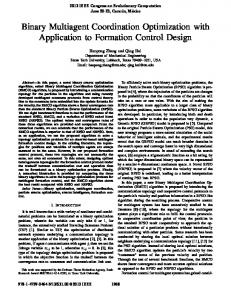
The aim of this chapter is to investigate the possibility of achieving the same control objective when only a very approximate knowledge of zk − zk∗ is available to the agents. Consider the component ` of zk − zk∗ , and suppose that the agent is only able to sense ∗ whether the actual inter-agent distance zk` is above or below the desired distance zk` and apply a control law to reduce or increase the actual distance. In mathematical terms, this control action has the form −bik sign(zk − zk∗ ), where sign y represents the vector (sign y1 . . . sign yp )T , and where the function sign : R → {−1, 1} is defined as sign(y) = +1 if y ≥ 0 and sign(y) = −1 if y < 0. To visualize such a sensing scenario, we present an example considering agents in a plane. Represent the position of the agents with respect to an inertial frame in R2 . Assign a local Cartesian coordinate system with an orientation identical to the inertial frame to each agent such that the current position of the agent is the origin of its local coordinate system. Therefore, each agent partitions the space R2 into four quadrants. Formally, the partition induced by the agent i, whose position with respect to the inertial frame is given by ri , is 4 [ represented by R2 = Qi , where i=1

Q1 Q2 Q3 Q4

= = = =

{r {r {r {r

∈ R2 ∈ R2 ∈ R2 ∈ R2

: r1 : r1 : r1 : r1

≥ ri1 , r2 < ri1 , r2 < ri1 , r2 ≥ ri1 , r2

≥ ri2 } ≥ ri2 } < ri2 } < ri2 }.

Our control scenario assumes that each agent i only detects the quadrant Qi in which the endpoint of the vector −bik (zk − zk∗ ) lies. Then, the controller √ of the agent i exerts the corresponding force along the bisector of Qi with magnitude 2. Thus, if the endpoint of −bik (zk −zk∗ ) lies in Q1 (see Fig. 3.1), then the control action is given by uik = −bik sign(zk − zk∗ ) (in the figure, it is denoted as uk for simplicity). We stress that any other vector whose endpoint lies in Q1 would return the same control value as the one due to −bik (zk − zk∗ ). Such a control scheme has several advantages, which we discuss below for the case in which p = 2. (i) Given any quadrant of the partition, the proposed control law returns the same control value for any vector −bik (zk − zk∗ ), corresponding to one of the neighbors of agent i, which lies in that quadrant. This shows that the formation is achieved even

3.1. Model and Motivation

23

−uk

Zk∗ Zk

uk

Zk − Zk∗

Figure 3.1: Agent i (bottom-left), a neighbor j (right) and the desired position of agent i with respect to agent j (top-left, in gray). Agent i detects the quadrant where zk − zk∗ and applies the control action −bik sign(zk − zk∗ ).

with large inaccuracies in the measurements of zk − zk∗ . In fact, the calculated control vector corresponding to a given vector −bik (zk − zk∗ ) is the same no matter where zk − zk∗ precisely lies in the quadrant. That is as far as the sign of zk − zk∗ is unchanged. (ii) If agent i detects that the vector zk − zk∗ is crossing the boundary of any two quadrants, then a new control vector is applied due to the term −bik sign(zk − zk∗ ). In our analysis below, however, we show that the exact formation is still achieved if this control vector at the boundary takes any value in the convex hull of the two control vectors associated with the two quadrants. More precisely, if zk − zk∗ = 0, then we allow for −bik sign(zk − zk∗ ) to take on any value in [−1, 1]2 (see (3.5) below). In this respect the control −(B ⊗ I2 )sign(˜ z) is robust to possible uncertainties in the precise detection of the boundary crossing. (iii) Neglecting the term −ki vi , the control ui takes on values in the following discrete set {−di , . . . , −1, 0, +1, . . . , +di } with di the degree of agent i. This means that if one replaces the damping term −ki vi with a bounded function, then the proposed control law implicitly includes saturation effects. (v) It contributes to the literature on quantized control systems showing that exact (and not practical as in other statically quantized control systems) convergence is achieved with extremely coarse information. In this respect it generalizes to higher-dimensional systems and to complex coordination tasks the results of [12, 17]. (vi) The proposed control law paves the way towards self-triggered coordination control [18]. Remark 3.1 Note that the assumption of identical Cartesian coordinate systems for the agents

3. Formation keeping control with binary controllers

24

of the network is to assist providing a clear explanation. In fact, the use of control law −(B ⊗ I2 )sign(˜ z ) for a network of double-integrators (point-masses) do not require this assumption. In the next section we are going to investigate the stability properties of the closed-loop system r˙i = vi m X (3.2) v˙ i = −kvi vi − kr bik sign(zk − zk∗ ), i = 1, . . . , n k=1

where kr , kvi are positive gains.

3.2

Results and Analysis

As a first step in the analysis we express the system (3.2) in the coordinates (˜ z , v), with z˜ = z − z ∗ . Thus z˜˙ = (B T ⊗ Ip )v (3.3) v˙ = −Kv v − kr (B ⊗ Ip )sign z˜ where Kv = diag(kv1 , . . . , kvn ) ⊗ Ip , and kvi , kr > 0. As a second step we define an appropriate notion of solutions. In fact, due to the discontinuous map sign z˜, the right-hand side of (3.3) is discontinuous. In this chapter, the solutions to the system above are intended in the Krasovskii sense. Let X = (˜ z , v) and F (X) be the set valued map F (X) =



(B T ⊗ Ip )v −Kv v



−



0 kr (B ⊗ Ip )



K sign z˜

(3.4)

p ˜k` and where K sign z˜ = ×m k=1 ×`=1 K sign z

Ksign z˜k` =



{sign z˜k` } [−1, 1]

if if

z˜k` 6= 0 z˜k` = 0.

(3.5)

We define X(t) = (˜ z (t), v(t)) a Krasovskii solution to (3.3) on the interval [0, t1 ] if it is an absolutely continuous function which satisfies the differential inclusion ˙ X(t) ∈ F (X(t))

(3.6)

for almost every t ∈ [0, t1 ], with F defined as in (3.4). Krasovskii solutions to the differential inclusion above always exist for sufficiently small values of t. In the following result we state the desired convergence property: Proposition 3.1 Any Krasovskii solution to (3.6) exists for all t ≥ 0 and converges to the origin. Proof: The proof is based on the application of the non-smooth La Salle’s invariance principle (see Chapter 2, Theorem 2.1). To this purpose we propose the function 1 V (˜ z , v) = kr ||˜ z ||1 + v T v 2

3.2. Results and Analysis

25

where ||˜ z ||1 denotes the 1-norm ||˜ z ||1 = ˙ V (˜ z , v) along (3.3). We have

P

k,`

|˜ zk` | and evaluate its set-valued derivative

V˙ (˜ z , v) = {a ∈ R : ∃w ∈ F (˜ z , v) s.t.a = hw, pi, for all p ∈ ∂V (˜ z , v)} By the definition of F (˜ z , v) in (3.4), for any w ∈ F (˜ z , v) there exists wz˜ ∈ Ksign z˜ such that     (B T ⊗ Ip )v 0 w= − wz˜. −Kv v kr (B ⊗ Ip ) Observe that the Clarke generalized gradient ∂V (˜ z , v) is given by ∂V (˜ z , v) = {p : p =



kr pz˜ v



˜ s.t.pzk`

∈



{sign z˜k` } [−1, +1]

z˜k` = 6 0 }. z˜k` = 0

if if

Suppose that V˙ (˜ z , v) 6= ∅ and take a ∈ V˙ (˜ z , v). Then by definition there exists w ∈ F (˜ z , v) such that a = hw, pi for all p ∈ ∂V (˜ z , v). In view of the definition of V , choose p ∈ ∂V (˜ z , v) such that pz˜ = wz˜. Thus a

= h



(B T ⊗ Ip )v −Kv v



−



0 kr (B ⊗ Ip )



z˜

w ,



kr wz˜ v



i

= h−Kv v, vi + h(B T ⊗ Ip )v, kr wz˜i − hkr (B ⊗ Ip )wz˜, vi = h−Kv v, vi. Hence, for any V˙ (˜ z , v) 6= ∅, V˙ (˜ z , v) = {−Kv ||v||2 } ⊆ (−∞, 0]. Hence, the solutions can be extended for all t ≥ 0 and by La Salle’s invariance principle they converge to the largest weakly invariant set where v = 0. From (3.4), any point (˜ z , 0) on this invariant set must necessarily satisfy   0 0= wz˜ kr (B ⊗ Ip ) for some wz˜ ∈ Ksign z˜. This implies wz˜ ∈ N (B⊗Ip ). Bearing in mind that z˜ ∈ R(B T ⊗Ip ), then h˜ z , wz˜i = 0. We claim that necessarily z˜ = 0. In fact, by contradiction, z˜ 6= 0 would imply the existence of at least a component z˜k` 6= 0. As z˜k` 6= 0 necessarily implies z˜ z˜ wk` 6= 0 by definition of wz˜ ∈ Ksign z˜, then it would imply z˜k` wk` > 0, which shows the contradiction. Hence, on the invariant set, z˜ = 0 and this ends the proof. Remark 3.2 (Finite-time convergence) In the case of single integrators, the use of signed controllers ( [13]) or control with signed measurements ( [12]) leads to finite-time convergence. It is not hard to find examples of system (3.3) for which finite-time convergence does not occur.

3. Formation keeping control with binary controllers

26

3.2.1

Saturated input

A natural modification of the control input proposed above, which could take into account a possible control saturation, is the following: u = −Kv sign v − kr (B ⊗ Ip )sign z˜. As a matter of fact, a similar analysis as for the proposition above yields that every Krasovskii solution converges to the largest weakly invariant set Z such that v = 0. Differently from the previous case, however, such a largest weakly invariant set strictly contains the origin. Proposition 3.2 Let p = 1.1 The largest weakly invariant set Z with respect to the following system z˜˙ = (B T ⊗ Ip )v (3.7) v˙ = −Kv sign v − kr (B ⊗ Ip )sign z˜ contains points such that for each agent i, vi = 0 and kr (card(Ni0 ) − card(N i0 )) ≥ −kvi where Ni0 corresponds to the neighbors of agent i which are at the desired inter-agent distance, while N i0 corresponds to the neighbors which are not. Proof: This can be shown remembering that for a point (˜ z , 0) to belong to the weakly invariant set it must be true that 0 = −Kv wv − kr (B ⊗ Ip )wz˜ for some wv ∈ Ksign0 and some wz˜ ∈ Ksign˜ z . Take for the sake of simplicity p = 1 and let z˜ 6= 0, then z˜k 6= 0 for some index k. Let i one of the two agents connected by the edge k. Then the component i of the identity above becomes 0 = −kvi wiv − kr

m X

bij wjz˜.

(3.8)

j=1

In the latter sum, let Ni0 be the set of indices j such that bij 6= 0 and z˜j = 0 and N i0 be the set of indices j such that bij 6= 0 and z˜j 6= 0. Ni0 is non empty by construction. Then write the equality as 0 = −kvi wiv − kr

m X

j∈Ni0

bij wjz˜ − kr

m X

bij wjz˜.

j∈N i0

Since wjz˜ ∈ {−1, +1} if j ∈ N i0 , the third term equals the product of an integer in the interval [−card(N i0 ), card(N i0 )] times kr . On the other hand, the sum of the first and second term takes any value in the interval [−(kvi + kr card(Ni0 )), (kvi + kr card(Ni0 ))]. Hence, provided that kr (card(Ni0 ) − card(N i0 )) ≥ −kvi the identity (3.8) is fulfilled. 1 The

case p > 1 does not change the analysis but complicates the notation.

3.3. Simulations

27

The latter result allows to conclude that the introduction of the discontinuous damping term −Kv sign v creates new undesired (Krasovskii) equilibria and should be avoided. To limit the velocity damping term, an intuitive alternative is to resort to a standard saturation function in the control input. In this case the control input becomes ui = −kvi sat vi − kr where sat : R → R is defined as sat r =



r 1

m X

k=1

bik sign(zk − zk∗ )

if if

r≤1 r > 1.

In the case r is a vector, the symbol sat r has to be intended component-wise. The closed-loop system becomes z˜˙ = v˙ =

(B T ⊗ Ip )v −Kv satv − kr (B ⊗ Ip )sign z˜

(3.9)

and in the associated differential inclusion (3.6) the set-valued map F is F (X) =



(B T ⊗ Ip )satv −Kv sat v



−



0 kr (B ⊗ Ip )



K sign z˜.

(3.10)

Then the following can be proven: Corollary 3.1 Any Krasovskii solution to (3.6) with F as in (3.10) exists for all t ≥ 0 and converges to the origin. Proof: Take the same function V used in the proof of Proposition 4.1. Following similar arguments one shows that any element a in V˙ (˜ z , v) is equal to a = h−K sat v, vi. v

As sat is a sector bound nonlinearity which lives in the first and third quadrant, V˙ (˜ z , v) ≤ ˙ 0 provided that V (˜ z , v) 6= ∅. This shows boundedness and existence for all t. Moreover,

by La Salle’s invariance principle, the solutions converge to the largest weakly invariant set where v = 0. This invariant set with respect to (3.10) is the same as the invariant set with respect to (3.4). The latter has been proven to coincide with (˜ z , v) = 0 and this ends the proof.

3.3

Simulations

In this section we present the simulation results for a group of five agents with unit mass and double integrator dynamics evolving in R2 . The simulation results are used to present numerical approximations of the behavior of the closed-loop system.

3. Formation keeping control with binary controllers

28

The agents are communicating over a connected graph. is  +1 0 0 0  −1 +1 0 0   B =  0 −1 +1 0   0 0 −1 +1 0 0 0 −1

The associated incidence matrix 

   .  

The desired formation has a pentagon shape with edge length equal to two and is defined √ T ∗ T ∗ by the following inter-agent position vectors: z = [0 − 2] , z = [−1 − 1 − 3] , 1 2 √ T ∗ ∗ T z3 = [−1 1 + 3] , z4 = [0 2] . Note that the number of edges of the graph is four. The initial position of the agents is set to r(0) = [0.5 − 0.5 0.5 1 1 0.5 0.8 0 1.1 0]T . Gains kr and Kv are equal to one and I2 . Figure 3.2 shows the evolution of the described system with desired constant velocity v ∗ = [0.6 0.6]T which is known to all of the agents. Figure 3.3 shows the time behavior of the horizontal component of z˜1 , sign z˜1 and the corresponding control u ˜1 . As time elapses, z˜1 converges to the origin implying convergence to the desired relative position. While z˜1 converges to zero, sign z˜1 and u ˜1 converge to the discontinuity surface and oscillate between +1 and −1. This fast switching behavior is a known undesired phenomenon due to the use of a sign-based controller [46]. In the next section, we study and propose solutions to deal with this problem.

14 12 10

Position−y (m)

8 6 4 2 trajectory of agent 1 trajectory of agent 2 trajectory of agent 3 trajectory of agent 4 trajectory of agent 5

0 −2 −4 0

2

4

6 8 Position−x (m)

10

12

14

Figure 3.2: The evolution of five agents in R2 tracking a constant reference velocity. The

system reaches the desired formation and exhibits a translational motion with the desired constant velocity.

3.4. Dealing with the fast switching controller

29

2

z˜11

1 0 −1

0

1

2

3

4

5

6

7

8

9

10

0

1

2

3

4

5

6

7

8

9

10

0

1

2

3

4

5

6

7

8

9

10

sign(˜z11 )

2

0

−2

u˜11

2

0

−2

Time (s)

Figure 3.3: The plot of the (horizontal) x-component of z˜1 , sign z˜1 and the corresponding

control u ˜1 .

3.4

Abstract— In this paper ....

Dealing with the fast switching controller I. CONCLUSIONS

In this section, we discuss the fast switching behavior of the control action u ¯ = −(B ⊗ ... I2 ) sign(˜ z ) as shown in Figure 3.3. Considering binary controllers, the aforementioned .............................................. phenomenon can be seen in simulation results of the next chapters. Here, we first explain the nature of the problem. Next, we propose three potential solutions to deal with the problem. The core of the proposed solutions are the same, that is, the injection of some dead-zone or inter-switching time in the structure of the controller and in the vicinity of the discontinuity surfaces. This thesis mainly focuses on strict (output) passive agents. A double-integrator dynamic agent is a simple example for strict passive agents. In this chapter, we analyze the fast switching behavior of the control action u ¯ designed to control the network in (3.3). The results of our analysis can be extended to the case of strict passive agents. First, we argue the nature of this fast oscillations to emphasis that the fast switchings correspond to the control action at the convergence of the state of the system to the origin. In fact, the convergence of solutions of system (3.3) is asymptotic (see Remark 3.2). Considering each discontinuity surface Si (˜ z ) = z˜k` = 0, the derivative of Si only depends on the velocity of the agents. Based on (3.3) and the proof of Proposition 3.1, the velocity of each agent is a continuous function which converges to zero asymptotically. This is different from the case of a network of single integrators with quantized control laws where it has been proven that the solutions may slide along discontinuity surfaces for some initial conditions [11]. We explain the fast switchings of the control action at the convergence of the solutions owing to the fact that the norm of −sign(˜ z ) on the discontinuity surfaces Si = 0 is always positive. In what follows, we propose three potential solutions to deal with this problem.

3. Formation keeping control with binary controllers

30

sh (x) B

-δ

+1

-1

δ

x

A

Figure 3.4: The illustration of map (3.12).

3.4.1

Hybrid-quantizer-based controllers

The first potential solution is based on the hybrid (hysteretic) quantizer introduced by [11] to deal with the chattering problem in a network of single integrators controlled by uniform quantizers. The underlying idea is to modify the structure of uniform quantizers such that each two quantization levels overlap. The latter prevent solutions to jump instantly from one level of discontinuity to another. Hence, preventing the undesired chattering of the solutions. We envision a similar improvement in fast oscillations of the control action in a network of double integrators (3.3) (and strictly passive systems) by adopting a hysteretic-quantizer-based design for sign function. In this thesis, we do not provide mathematical analysis for the network of double integrators with the new modifications in the design of the controller. But we present the proposed controller and the related simulation results. The analysis requires the use of hybrid systems formalism and is one of the candidates for future developments. We introduce the multi- valued sign function, sh (x), as follows

sh (x) =

 

+1 −1  {−1, +1}

x>δ x ε |˜ zk` | ≤ ε

Evaluating the set-valued derivative V˙ (˜ z , v) along (3.14), we have V˙ (˜ z , v) = {a ∈ R : ∃w ∈ F (˜ z , v) s.t. a = hw, pi, for all p ∈ ∂V (˜ z , v)}.

(3.17)

34

3. Formation keeping control with binary controllers

By the definition of F (˜ z , v) in (3.15), for any w ∈ F (˜ z , v) there exists wz˜ ∈ K signε z˜ such that     (B T ⊗ I2 )v 0 w= − wz˜. −kv (B ⊗ I2 )

Observe that the Clarke generalized gradient ∂V (˜ z , v) is given by   z˜   {signε z˜k } if z˜k 6= ε p ∂V (˜ z , v) = {p : p = s.t. pzk˜ ∈ [0, +1] if z˜k = ε }.  v [−1, 0] if z˜k = −ε

Suppose that V˙ (˜ z , v) 6= ∅ and take a ∈ V˙ (˜ z , v). Then by definition there exists w ∈ F (˜ z , v) z˜ z˜ such that a = hw, pi for all p ∈ ∂V (˜ z , v). Choose p ∈ ∂V (˜ z , v) such that p = w . Thus       (B T ⊗ I2 )v 0 wz˜ a=h − wz˜, i = h−k||v||2 i. −kv (B ⊗ I2 ) v

Therefore, V˙ (˜ z , v) = {−k||v||2 } ⊆ (−∞, 0]. Hence, the solutions can be extended for all t ≥ 0 and by La Salle’s invariance principle they converge to the largest weakly invariant set where v = 0. From (3.15), v = 0 implies that (B ⊗ I2 )wz˜ = 0 and consequently wz˜ ∈ N (B ⊗ I2 ). Since, z˜ ∈ R(B T ⊗ I2 ), then we conclude that on the set S in (3.13), h˜ z , wz˜i = 0 should hold. We claim that necessarily |˜ zk` | ≤ ε for all k and wz˜ = 0. By, z˜ contradiction, |˜ zk | > ε would necessarily imply wk`,i 6= 0 by definition of wz˜ ∈ Ksign z˜, then it would imply z˜k wkz˜ > 0, which shows the contradiction. A similar reasoning requires wz˜ = 0. Based on the above result, the connectivity of the graph requires that the equality h˜ z , wz˜i = 0 holds on the weakly invariant set S (as defined in (3.13)). Since wz˜ = 0, the control action of each agent i should be equal to zero on S. Considering the set S and points |˜ zk` | = ε belong to S, we conclude that small perturbations on these points result in |˜ zk` | < ε. Note that a subset of S such that |˜ zk` | is strictly smaller than ε for all k, ` is strongly invariant with respect to (3.3). Figure 3.7 shows the simulation results of a network of five double integrators in R2 communicating over a connected undirected graph as in Section 3.3. The constants ε and k are equal to 0.2 and 1 respectively. Note that ε is a design choice and it should be chosen big enough, for example in the simulations, it is taken bigger than the relative tolerance of the integration method. The results show the convergence of the network to a formation for which |˜ zk` | < ε while the velocity of each of the agents converges to zero. As expected, the control action does not show fast switchings at the convergence. Despite a chattering-free convergence, given a desired ε, the fast switching of the control action can initially occur for some graph topologies, specific initial conditions and damping coefficient k. Here, we provide an example in agents evolving in R (for the sake of simplicity). Example 3.1 Consider a connected graph composed of three nodes and two links. Take z ∗ = 0, then we have z˜ = z. Define z1 = x2 − x1 and z2 = x3 − x2 such that z1 (0) = ε, z2 (0) > ε and

3.4. Dealing with the fast switching controller

35

z˜x(m)

1

0.2 0 −0.2 0

2

4

6

8

10

12

14

16

18

20

−1 0

2

4

6

8

10

12

14

16

18

20

2

4

6

8

10

12

14

16

18

20

vx(m/s)

1

0

u11

2

0

−2 0

Time (s)

Figure 3.7: The plots of relative position error and velocity of the agents in x-direction, z˜x

and vx , together with the controller of the first agent in x-direction, u11 . v(0) = 0. Calculating the evolution of z˙1 on the small time interval [0, δ], we obtain z˙1 = v2 − v1 = t − 2 signε (z1 (0)) t. Hence, limz1 →ε− z˙1 = t and limz1 →ε+ z˙1 = −t. The change of sign of z˙1 around z1 = ε implies initial oscillations. The oscillations will disappear while the system converges to the desired formation.

3.4.3

Self-triggered coordination algorithms

The last proposed method relies on event-based control techniques. In the case of networks of kinematic agents, the finite-valued control law of [13] inspired the design of self-triggered control algorithms (see [18]). The underlying idea is the following. If it is possible to achieve coordination via binary information, then the controller only needs to keep track of the times when the measured information crosses zero. If one can predict when these time instants occur, and make sure that they do not accumulate in finite time, then the control will be updated only at these instants, thus preventing the occurrence of the fast switching behavior. The effectiveness of the above method in dealing with the chattering for a network of single-integrators and double-integrators can be found in [18] and [22] respectively. Chapter 6 of this thesis analyzes the self-triggered algorithm in [18] within the hybrid formalism.

3. Formation keeping control with binary controllers

36

3.5

Conclusions

This chapter has presented motivational results on the formation keeping control using binary information and control which will be studied further in the next chapters. A network of double integrators over a connected and undirected graph has been considered together with linear and nonlinear velocity feedbacks. The agents are assumed to exchange very coarse information. It has been shown that the exact desired formation can be achieved despite binary exchanged data. However, the application of binary controllers introduce fast switchings of the control action at the convergence. This chapter has also studied the latter problem and proposed different solutions which are interesting for future investigations. In conclusion, the problem of fast oscillations can be mitigated with some improvements in the design of the controllers allowing the binary controllers to retain their main advantage, that is achieving complex tasks with simple commands and without the need of perfect information.

Chapter 4

Formation control, velocity tracking and disturbance rejection using binary controllers Motivated by Chapter 3, this chapter studies the problem of distributed position-based formation keeping of a group of agents with strictly passive dynamics which exchange binary information. Remarkably, despite such a coarse information scenario and control laws, we show that the control law guarantees exact achievement of the desired formation. Moreover, this chapter investigates the formation control problem together with tracking known and unknown reference velocities. We prove that the formation tracks a desired reference velocity even when the reference velocity is only available to one of the agents (the so-called leader). In addition, the matched input disturbance rejection is studied considering both harmonic and constant disturbances. The results of this chapter have been published in [46]. The outline of this chapter is as follows. Section 4.1 introduces the problem formulation. Analysis of the formation keeping problem with binary controllers in the case of known/unknown reference velocity is studied in Section 4.2. Section 4.3 investigates the problem of formation keeping with binary controllers in the presence of matched input disturbances. Related simulations are presented in Section 4.4. This chapter is summarized in Section 4.5.

4.1

Problem Formulation

We assume that the velocity of each agent is given by x˙ i = Hi {ui } + vir ,

(4.1)

where Hi {ui } represents a system with dynamics (as in Fig. 4.1) Hi :

(

ξ˙i = fi (ξi ) + gi (ξi )ui yi = hi (ξi )

(4.2)

where ξi ∈ Rni is the state variable, ui ∈ Rp is the control input, yi ∈ Rp is the velocity error, and the exogenous signal vir ∈ Rp is the reference velocity for agent i. The maps fi , gi and hi are assumed to be locally Lipschitz such that fi (0) = 0, hi (0) = 0, and gi (0) is full column-rank.

     

38

4. Formation control, velocity tracking and disturbance rejection using binary controllers  

 

.  

 

 

 

+ 

.

+

.  

Figure 4.1: The dynamics of each agent is assumed to be composed of a strictly passive system and an integrator. The system Hi is strictly passive from an external input ui to the velocity error yi .

Notice that the output yi of (4.2) is the velocity tracking error x˙i − vir , namely yi = x˙i − vir .

(4.3)

The system Hi is assumed to be strictly passive from the input ui to the velocity error yi . For the sake of conciseness, the equations (4.2) and (4.3) are written in the compact form 

  r  h1 (ξ1 ) v1    . .  .. x˙ =   +  ..  r hN (ξN ) vN | {z } | {z } h(ξ)

vr

 g1 (ξ1 ) . . . 0 f1 (ξ1 )     .. .. .. .. ξ˙ =  u + . . . . 0 . . . gN (ξN ) fN (ξN ) {z } | {z } | 

f (ξ)





(4.4)

g(ξ)

y = h(ξ).

We define the concatenated vectors x , [xT1 . . . xTN ]T , x ∈ RpN , xi ∈ Rp , and ξ , T T [ξ1T . . . ξN ] , ξ ∈ RpN , ξi ∈ Rp . The desired position x∗ , with x∗ , [x∗1 T . . . x∗N T ]T , Rt x∗ ∈ RpN , x∗i ∈ Rp is given by x∗ = x∗0 + 1N ⊗ 0 v ∗ (s)ds, with x∗0 a constant vector. ∗ T T Analogously, z ∗ , [z1∗ T . . . zM ] , z ∗ ∈ RpM , zi∗ ∈ Rp , is the desired relative position vector. The two vectors are related by the identity z ∗ = (B T ⊗ Ip )x∗ . Our goal is to design coordination control laws to attain the following collective behaviors for the formation of dynamic agents (4.2), (4.3): (i) The velocity of each agent of the network asymptotically converges to the desired reference velocity v ∗ (t) ∈ Rp lim ||x˙i (t) − v ∗ (t)|| = 0, i = 1, ..., N.

t→∞

(4.5)

(ii) Each relative position vector zk converges to the desired relative position vector zk∗ lim ||zk − zk∗ || = 0, zk∗ ∈ Rp , k = 1, ..., M.

t→∞

(4.6)

4.2. Analysis

39

(iii) In the presence of matched disturbances, i.e. in the case in which the equation (4.2) is replaced by ξ˙i = fi (ξi ) + gi (ξi )(ui + di ) where di is a disturbance signal generated by a suitable exosystem (see Section 4.3), the collective behaviors in (i) and (ii) are still guaranteed. Differently from other work in formation control, we are interested in control laws that achieve complex coordination tasks using very coarse information about the relative positions of the agents. We assume that the agents of the network are equipped with sensors that are capable to detect whether the relative position of two agents is above or below a prescribed one. In line with our goals, for each agent i, the control law is designed as M X ui = − bik sign(zk − zk∗ ), i = 1 ... N, (4.7) k=1

where sign(·) is the sign function and operates on each element of the p-dimensional vector zk − zk∗ . The sign function sign(·) : R → {−1, +1} is defined as follows sign(ζ) =



+1 if −1 if

ζ≥0 ζ < 0.

Observe that, bik 6= 0 if and only if the edge k connects agent i to one of its neighbors. This implies the control law ui uses only the information available to agent i. The above control law is inspired by the passivity-based control design proposed in [1] and has been motivated in Chapter 3.

4.2

Analysis

In this section we investigate the stability properties of the closed-loop system. We define the error variable z˜ = z − z ∗ and write the control laws ui , i = 1, 2, . . . , N , in the following compact form u = −(B ⊗ Ip )sign z˜.

(4.8)

From (2.1), we can write z˜ = (B T ⊗ Ip )(x − x∗ ). We consider the stability of the origin of the error system, with state variable (˜ z T , ξ T )T . To derive the error system equations, we take the derivative of z˜, thus obtaining z˜˙ = (B T ⊗ Ip )(x˙ − x˙ ∗ ).

(4.9)

From equation (4.4), we further have x˙ − x˙ ∗ = h(ξ) + v r − 1N ⊗ v ∗

(4.10)

40

4. Formation control, velocity tracking and disturbance rejection using binary controllers

where v ∗ is the desired reference velocity for the formation. By a property of the incidence matrix of a connected graph, (B T ⊗ Ip )(1N ⊗ v ∗ ) = 0. Thus, we represent the dynamics of the error system in the following general form z˜˙ = (B T ⊗ Ip )x˙ = (B T ⊗ Ip )(h(ξ) + v r )

(4.11)

ξ˙ = f (ξ) + g(ξ)(−B ⊗ Ip ) sign z˜.

The system (4.11) has a discontinuous right-hand side due to the discontinuity of the sign function at zero. Before analyzing the system, we first define an appropriate notion of the solution. Similar to Chapter 3, in this chapter, the solutions to the system above are intended in the Krasovskii sense. As in [11, 20], the motivation to consider these solutions lies in the fact that there exist convenient Lyapunov methods to analyze their asymptotic behavior and that they include other notions of solutions such as Carath´eodory solutions if the latter exists. Let X = (˜ z , ξ) and let F (X) be the set-valued map F (X) =



(B T ⊗ Ip)(h(ξ) + v r ) f (ξ)



−



0 g(ξ)(B ⊗ Ip)



Ksign z˜

(4.12)

p where K sign z˜ = ×M ˜k` and k=1 ×`=1 K sign z

K sign z˜k` =



{sign z˜k` } [−1, 1]

if if

z˜k` 6= 0 z˜k` = 0.

(4.13)

We define X(t) = (˜ z (t), ξ(t)) a Krasovskii solution to (4.11) on the interval [0, t1 ] if it is an absolutely continuous function which satisfies the differential inclusion ˙ X(t) ∈ F (X(t))

(4.14)

for almost every t ∈ [0, t1 ], with F defined as in (4.12). Notice that the relation between the differential inclusion (4.14) and the discontinuous ordinary differential equations (4.11) stems from the property K(f (X)) =

\

δ>0

co(f (B(x, δ))) ⊆ F (X),

(4.15)

with f (X) the map defining the right-hand side of (4.11), co the closed convex hull of a set and B(x, δ) the ball centered at x and of radius δ. Local existence of Krasovskii solutions to the differential inclusion above is always guaranteed (see e.g. [37] and [11], Lemma 3).

4.2.1

Known reference velocity

In this section, we consider the case where the desired reference velocity, v ∗ (t), is known to all the agents, namely v r = 1N ⊗ v ∗ .

4.2. Analysis

41

Proposition 4.1 Any Krasovskii solution to the closed-loop system z˜˙ = (B T ⊗ Ip )h(ξ)

(4.16)

ξ˙ = f (ξ) + g(ξ)(−B ⊗ Ip )sign z˜ exists for all t ≥ 0 and converges to the the point z˜ = 0, ξ = 0.

Proof: Since v r = 1N ⊗ v ∗ , the closed-loop system in (4.11) simplifies to (4.16). Local existence of Krasovskii solutions is guaranteed by the fact that the right hand side of (4.16) is measurable and locally bounded (i.e., bounded on each bounded subset of its domain [37]). Moreover, completeness of solutions can be deduced by their boundedness ( [60]). Boundedness of solutions to system (4.16) is proven below (see [20], Lemma 3.1, Theorem 3.2 for more details), thus showing completeness. The convergence proof is based on the application of the nonsmooth La Salle’s invariance principle (see Chapter 2, Theorem 2.1). Consider the following locally Lipschitz Lyapunov function V (˜ z , ξ) = ||˜ z ||1 + S(ξ) P where ||˜ z ||1 denotes the 1-norm ||˜ z ||1 = k,` |˜ zk` | and evaluate its set-valued derivative ˙ V (˜ z , ξ) along (4.16). We have V˙ (˜ z , ξ) = {a ∈ R : ∃w ∈ F (˜ z , ξ) s.t. a = hw, pi, for all p ∈ ∂V (˜ z , ξ)}. By the definition of F (˜ z , ξ) in (4.12), for any w ∈ F (˜ z , ξ) there exists wz˜ ∈ Ksign z˜ such that     (B T ⊗ Ip )h(ξ) 0 w= − wz˜. f (ξ) g(ξ) (B ⊗ Ip ) Observe that the Clarke generalized gradient ∂V (˜ z , ξ) is given by    pz˜ {sign z˜k` } if ˜ ∂V (˜ z , ξ) = {p : p = s.t. pzk` ∈ ∇S(ξ) [−1, +1] if

z˜k` = 6 0 }. z˜k` = 0

Suppose that V˙ (˜ z , ξ) 6= ∅ and take a ∈ V˙ (˜ z , ξ). Then by definition there exists w ∈ F (˜ z , ξ) such that a = hw, pi for all p ∈ ∂V (˜ z , ξ). Choose p ∈ ∂V (˜ z , ξ) such that pz˜ = wz˜. Thus,  T      (B ⊗ Ip )h(ξ) 0 wz˜ a = h − wz˜, i f (ξ) g(ξ) (B ⊗ Ip ) ∇S(ξ) = h(B T ⊗ Ip)h(ξ), wz˜i + hf (ξ) − g(ξ)(B ⊗ Ip)wz˜, ∇S(ξ)i ≤

−W (ξ).

Hence, for any state (˜ z , ξ) such that V˙ (˜ z , ξ) 6= ∅, V˙ (˜ z , ξ) = {a ∈ R : a ≤ −W (ξ)} ⊆ (−∞, 0]. Therefore, the solutions can be extended for all t ≥ 0 and by La Salle’s invariance principle they converge to the largest weakly invariant set where ξ = 0. Since v r = 1N ⊗v ∗ , from (4.12), any point (˜ z , 0) on this invariant set must necessarily satisfy   0 0= wz˜ g(0)(B ⊗ Ip )

42

4. Formation control, velocity tracking and disturbance rejection using binary controllers

for some wz˜ ∈ Ksign z˜. Since g(0) is full-column rank, this implies wz˜ ∈ N (B ⊗ Ip ). Bearing in mind that z˜ ∈ R(B T ⊗ Ip ), then h˜ z , wz˜i = 0. We claim that necessarily z˜ = 0. In fact, by contradiction, z˜ 6= 0 would imply the existence of at least a component z˜k` 6= 0. z˜ As z˜k` 6= 0 necessarily implies wk` 6= 0 by definition of wz˜ ∈ Ksign z˜, then it would imply z˜ z˜k` wk` > 0, which shows the contradiction. Hence, on the invariant set, z˜ = 0 and all the system’s solutions converge to the origin.

4.2.2

Unknown reference velocity

In the previous section, we assumed that the desired reference velocity is known to all of the agents. This assumption is very restrictive and one wonders whether it is possible to relax this assumption despite the very coarse information scenario we are confining ourselves. The positive answer to this question is given in the analysis below. The problem of the reference velocity unknown to the agents is tackled here in the scenario in which at least one of the agents is aware of v ∗ . We refer to this agent as the leader ( [56], [68]). As in [4], we further assume that the class of reference velocities that the formation can achieve are those generated by an autonomous system that we refer to as the exosystem. Given two matrices Φ, Γv , whose properties will be made precise later on, the exosystem obeys the following equations w˙v = Φwv ,

v ∗ = Γv wv .

(4.17)

Taking inspiration from the theory of output regulation (see e.g. [39]), an internal-modelbased controller can be adopted for each agent i = 2, 3, . . . , N , namely η˙ i vir

= Φηi + G˜ ui v = Γ ηi ,

i = 2, 3, . . . , N.

(4.18)

When u ˜i = 0 and the system is appropriately initialized, the latter system is able to generate any wv solution to (4.17). Because v ∗ is known to agent 1, there is no need to implement system (4.18) at agent 1. The input u ˜i , as well as the input matrix G are to be r ∗T r T r T designed later. Define v = (v v2 . . . vN ) and the new error variables η˜i = ηi − wv ,

v˜i = vir − v ∗ ,

i = 2, . . . , N,

along with the fictitious variables η˜1 = 0, v˜1 = 0. In compact form, we obtain η˜˙ = v˜ =

˜ η + G˜ ˜u Φ˜ v ˜ η˜, Γ

(4.19)

˜ G, ˜ and Γ ˜ v are Φ ˜ = block.diag{0, Φ, . . . , Φ}, G ˜ = block.diag{0, G, . . . , G}, Γ ˜v = where Φ, v v block.diag{0, Γ , . . . , Γ }. From (4.11), the error position vector can be written as z˜˙ = = =

(B T ⊗ Ip )(h(ξ) + v r ) (B T ⊗ Ip )(h(ξ) + v r − 1N ⊗ v ∗ + 1N ⊗ v ∗ ) (B T ⊗ Ip )(h(ξ) + v˜).

4.2. Analysis

43

The overall closed-loop system is ˜ v η˜) z˜˙ = (B T ⊗ Ip )(h(ξ) + Γ ˙ξ = f (ξ) + g(ξ)u ˜ η + G˜ ˜ u. η˜˙ = Φ˜

(4.20)

Proposition 4.2 Assume that Φ is skew-symmetric, namely ΦT + Φ = 0,

(4.21)

G = Γv T .

(4.22)

(Γv , Φ) is an observable pair and let

Then all the Krasovskii solutions to (4.20) in closed-loop with the control input u=u ˜ = −(B ⊗ Ip )sign z˜

(4.23)

converge to the point z˜ = 0, ξ = 0, η˜ = 0. Proof: Any Krasovskii solution to (4.20) with the control law defined by (4.23) satisfies a differential inclusion of the form (4.12) where X = (˜ z , ξ, η˜) and F (X) is equal to   ˜ v η˜)   (B T ⊗ Ip )(h(ξ) + Γ 0   −  g(ξ)(B ⊗ Ip )  K sign z˜. f (ξ) ˜η ˜ ⊗ Ip ) Φ˜ G(B Let

1 V (˜ z , v˜, η˜) = ||˜ z ||1 + S(ξ) + η˜T η˜. 2

For any w ∈ F (˜ z , ξ, η˜), there exists wz˜ ∈ Ksign z˜ such that 

 ˜ v η˜)   (B T ⊗ Ip )(h(ξ) + Γ 0  −  g(ξ)(B ⊗ Ip )  wz˜. w= f (ξ) ˜η ˜ (B ⊗ Ip ) Φ˜ G

Moreover for any p ∈ ∂V (˜ z , ξ, η˜) there exists pz˜ ∈ ∂||˜ z ||1 , with ˜ pzk` ∈



{sign z˜k` } [−1, +1]

if if

z˜k` = 6 0 z˜k` = 0,

and k = 1, 2, . . . , M , ` = 1, 2, . . . , p, such that 

 pz˜ p =  ∇S(ξ)  . η˜

44

4. Formation control, velocity tracking and disturbance rejection using binary controllers

For wz˜ ∈ Ksign z˜, let p ∈ ∂V (˜ z , ξ, η˜) such that wz˜ = pz˜. Hence, ˜ v η˜), wz˜i hw, pi = h(B T ⊗ Ip )(h(ξ) + Γ +hf (ξ) − g(ξ)(B ⊗ Ip )wz˜, ∇S(ξ)i ˜η − G ˜ (B ⊗ Ip )wz˜, η˜i. +hΦ˜ By (4.21) and (4.22), the equality above simplifies as hw, pi = h(B T ⊗ Ip )h(ξ), wz˜i + hf (ξ) − g(ξ)(B ⊗ Ip )wz˜, ∇S(ξ)i. Since the dynamic of each agent is strictly passive, we have hf (ξ) − g(ξ)(B ⊗ Ip)wz˜, ∇S(ξ)i ≤ −W (ξ) − hh(ξ), (B ⊗ Ip)wz˜i which implies hw, pi ≤ −W (ξ).

Hence, similarly to the proof of Proposition 4.1, V˙ (˜ z , ξ, η˜) = {a ∈ R : a ≤ −W (ξ)} ⊆ z , ξ, η˜) 6= ∅. Because V is positive definite and proper, solutions (−∞, 0], provided that V˙ (˜

are bounded and one can apply La Salle’s invariance principle which shows that every Krasovskii solution converges to the largest weakly invariant set where W (ξ) = 0. By definition of W (ξ), the latter is equivalent to have convergence to the largest weakly invariant set where ξ = 0. To characterize this set, we look for points (˜ z , 0, η˜) such that ˙ ˙ (z˜, 0, η˜) ∈ F (˜ z , 0, η˜). Having f (0) = h(0) = 0, this means that we seek points (˜ z , 0, η˜) for which there exists wz˜ ∈ K sign z˜ such that  ˙    ˜ v η˜)   (B T ⊗ Ip )(Γ 0 z˜ 0=  −  g(0)(B ⊗ Ip )  wz˜. 0 ˜η ˜ v )T (B ⊗ Ip ) η˜˙ Φ˜ (Γ

The equality 0 = −g(0)(B ⊗ Ip )wz˜, implies that necessarily z˜ = 0 (see the final part of the proof of Proposition 4.1). This also implies that on the invariant set the system evolves as ˜ v η˜) 0 = (B T ⊗ Ip )(Γ ˜ η. η˜˙ = Φ˜ From this point on, the argument is the same as in [4]. Indeed, as N (B T ) = R(1N ), by ˜ v , we obtain that all the sub vectors of Γ ˜ v η˜ must be the the block diagonal structure of Γ ˜ v η˜ are identically zero. In other same and equal to zero, since the first p components of Γ v words, Γ η˜i = 0 for all i = 2, 3, . . . , N . Hence we conclude that on the largest weakly invariant set where ξ = 0, we have 0 = Γv η˜i ˙η˜i = Φ˜ ηi ,

i = 2, 3, . . . , N.

By the observability of (Γv , Φ), it holds that η˜i = 0 for all i = 2, 3, . . . , N . This finally proves the claim.

4.3. Formation control with matched disturbance rejection

4.3

45

Formation control with matched disturbance rejection

In this section, we study the problem of formation keeping with binary controllers in the presence of matched input disturbances. We consider a formation of strictly passive agents, where the dynamics of each agent of the network is x˙ i = yi + vir (t)

Hi :

(

ξ˙i = fi (ξi ) + gi (ξi )(ui + di ) yi = hi (ξi ),

(4.24)

where di is a disturbance. The network should converge to the prescribed formation and evolve with the given desired reference velocity v ∗ despite the action of the disturbance d. As in the previous section, we first consider the case in which the reference velocity is unknown to all the agents except one. As explained in Section 4.2.2, we adopt an internal-model-based controller to recover the desired reference velocity. Similarly we suppose that the disturbance signal di at agent i is generated by an exosystem of the form w˙ id = Φdi wid ,

di = Γdi wid ,

i = 1, 2, . . . , N.

(4.25)

To counteract the effect of the disturbance, we introduce an additional internal-modelbased controller given by θ˙i dˆi

= Φdi θi + Gdi u ˇi = Γdi θi ,

i = 1, 2, . . . , N,

(4.26)

where Gdi , u ˇi will be designed later. We remark that the internal model for disturbance rejection is implemented also by agent 1 (the leader). To both compensate the disturbance and achieve the desired formation, the proposed control law is composed of two parts: u ˆ guides the system to the desired formation, and dˆ compensates the disturbance. Therefore, we can write the dynamics of the agents in the following compact form u=u ˆ − dˆ (4.27) ξ˙ = f (ξ) + g(ξ)(ˆ u − dˆ + d). Define the new variable d˜i = dˆi − di and θ˜i = θi − wid , then ˙ θ˜i = Φdi θ˜i + Gdi u ˇi d d˜i = Γi θ˜i .

(4.28)

˙ θ˜ = Φd θ˜ + Gd u ˇ ˜ d˜ = Γd θ,

(4.29)

In compact form we write

where the matrices Φd , Gd , and Γd are diagonal matrices whose diagonal elements are Φdi , Gdi , and Γdi respectively.

46

4. Formation control, velocity tracking and disturbance rejection using binary controllers

From the equation (4.20) together with the equations (4.27) and (4.29), the overall closed-loop system is ˜ v η˜) z˜˙ = (B T ⊗ Ip )(h(ξ) + Γ ˜ ξ˙ = f (ξ) + g(ξ)(ˆ u − Γd θ) (4.30) ˜ η + G˜ ˜u ˙η˜ = Φ˜ ˙ θ˜ = Φd θ˜ + Gd u ˇ. The following is proven: Proposition 4.3 Assume that Φ and Φdi , for i = 1, 2, . . . , N are skew-symmetric matrices. If G = (Γv )T Gdi = (Γdi )T ,

(4.31)

then all the Krasovskii solutions to (4.30) in closed-loop with the control input u ˆ=u ˜ = −(B ⊗ Ip )sign˜ z,

u ˇ = h(ξ)

are bounded and converge to the largest weakly invariant set for    ˜ v η˜ z˜˙ (B T ⊗ Ip )Γ  0   −(B ⊗ Ip )K sign˜ z − Γd θ˜    ˙ ∈ v T  ˜ ˜ Φ˜ η − (Γ ) (B ⊗ Ip )K sign˜ z  η˜  ˙ d˜ ˜ θ Φ θ

such that ξ = 0.

(4.32) 

 , 

(4.33)

Proof: Consider the Lyapunov function 1 ˜ 1 ˜ = ||˜ V (˜ z , ξ, η˜, θ) z ||1 + S(ξ) + η˜T η˜ + θ˜T θ. 2 2 Any Krasovskii solution to (4.30) with the control law defined by (4.32) satisfies a differ˜ and F (X) is ential inclusion of the form (4.14) where X = (˜ z , ξ, η˜, θ)   ˜ v η˜)   (B T ⊗ Ip )(h(ξ) + Γ 0    g(ξ)(B ⊗ Ip )  f (ξ) − g(ξ)Γd θ˜  −     G(B ˜ ˜ ⊗ Ip )  K sign z˜. Φ˜ η 0 Φd θ˜ + Gd h(ξ) For any w ∈ F (X), there exists wz˜ ∈ Ksign z˜ such that  ˜ v η˜)   (B T ⊗ Ip )(h(ξ) + Γ 0 d˜    g(ξ)(B ⊗ Ip ) f (ξ) − g(ξ)Γ θ − w=    G(B ˜η ˜ ⊗ Ip ) Φ˜ 0 Φd θ˜ + Gd h(ξ) ˜ there exists pz˜ ∈ ∂||˜ Moreover for any p ∈ ∂V (˜ z , ξ, η˜, θ) z ||1 , with  {sign z˜k` } if z˜k` 6= 0 ˜ pzk` ∈ [−1, +1] if z˜k` = 0,



 z˜ w . 

4.3. Formation control with matched disturbance rejection

47

and k = 1, 2, . . . , M , ` = 1, 2, . . . , p, such that  pz˜  ∇S(ξ)  . p=   η˜ ˜ θ 

˜ be such that wz˜ = pz˜. Hence, For wz˜ ∈ Ksign z˜, let p ∈ ∂V (˜ z , ξ, η˜, θ) ˜ v η˜), wz˜i hw, pi = h(B T ⊗ Ip )(h(ξ) + Γ ˜ ∇S(ξ)i + hf (ξ) − g(ξ)((B ⊗ Ip )wz˜ + Γd θ), ˜ ˜η − G ˜ (B ⊗ Ip )wz˜, η˜i + hΦd θ˜ + Gd h(ξ), θi. + hΦ˜ By condition (4.31), the above result simplifies as hw, pi = h(B T ⊗ Ip )h(ξ), wz˜i ˜ ∇S(ξ)i + hf (ξ) − g(ξ)((B ⊗ Ip )wz˜ + Γd θ),

(4.34)

˜ + hGd h(ξ), θi. Since the dynamics of each agent is strictly passive, we have ˜ ∇S(ξ)i ≤ −W (ξ) − hh(ξ), (B ⊗ Ip )wz˜ + Γd θi. ˜ hf (ξ) − g(ξ)((B ⊗ Ip )wz˜ + Γd θ), When it is replaced in (4.34), it gives hw, pi ≤ −W (ξ), in view of Γd = (Gd )T . As in the ˜ = {a ∈ R : a ≤ −W (ξ)} and hence boundedness previous proofs, this shows V˙ (˜ z , ξ, η˜, θ)

of the solutions and their convergence to the largest weakly invariant set for the closedloop system such that ξ = 0. This proves the thesis. Remark 4.1 The disturbance rejection controller for each agent i only uses the local information yi = hi (ξi ), despite the fact that the disturbance affects the input through which agent i coordinates with the other agents in the network. Note that the input of each agent is only influenced by a function of its own velocity gi (ξi ) (see Equation (4.4)).

Proposition 4.3 only proves boundedness of the solution and convergence of the velocity of each agent to its own reference velocity (ξ = 0). To prove the convergence of the network to the desired formation and evolution of the network with the desired velocity, one should additionally prove that z˜ converges to the origin. This result does not hold in general but there are a few cases of interest where this is true. In what follows we study two of these cases. Case I: Φ = 0, Φdi = 0p×p , i = 1, 2, . . . , N , and Γv , Γdi , i = 1, 2, . . . , N , are nonsingular. This case corresponds to the scenario in which the unknown reference velocity and the disturbances are constant signals. The arguments below show that the distributed control laws characterized in Proposition 4.3 guarantee the achievement of the desired formation

48

4. Formation control, velocity tracking and disturbance rejection using binary controllers

and the prescribed velocity while rejecting the disturbances. From Proposition 4.3 it is known that the system converges to the largest weakly invariant set for (4.33) such that ξ = 0. In the case Φ = 0, Φdi = 0p×p , this implies that ˜ = (˜ ˜ on this set, and for any w ∈ F (˜ ˜ there exists for any state (˜ z , ξ, η˜, θ) z , 0, η˜, θ) z , ξ, η˜, θ), z˜ w ∈ K sign z˜, such that ˜ v η˜) z˜˙ = (B T ⊗ Ip )(Γ 0 = −(B ⊗ Ip )wz˜ − Γd θ˜ (4.35) ˜ v )T (B ⊗ Ip )wz˜ η˜˙ = −(Γ ˙ θ˜ = 0. ˙ From θ˜ = 0, we conclude that θ˜ is a constant vector. Hence, considering the second equality in (4.35), we conclude that (B ⊗ Ip )wz˜ is a constant vector. From the third equation, we deduce that each component of η˜˙ (t) is identically zero. As a matter of fact, the first component is zero by construction. The vectors η˜˙ i (t), i = 2, . . . , N , are constant. If η˜˙ i (t) is a non-zero vector for some i, then at least one of its components, say η˜˙ i` (t), must be non-zero and then η˜i` (t) would grow with constant velocity and this would contradict the boundedness of the solutions. Hence, η˜˙ (t) = 0 and η˜(t) is a constant vector. From the first equation, the latter implies that z˜˙ (t) is constant as well. The same argument used for η˜˙ (t) can be used again to show that z˜˙ (t) = 0. Now, consider the first equality in (4.35) and multiply both sides by B ⊗ Ip . Since z˜˙ = 0, we obtain ˜ v η˜). From the property of the Laplacian of a connected undirected 0 = (BB T ⊗ Ip )(Γ ˜ v η˜ = R(1N ⊗ Ip ). From the definition of Γ ˜ v η˜, we have Γ ˜ v η˜ = 0 and graph, we conclude Γ v ˜ ˙ hence η˜ = 0. The third identity in (4.35), η˜ = 0, and the structure of Γ implies that (B ⊗ Ip )wz˜ =



B1T ⊗ Ip B2T ⊗ Ip



wz˜ =



c 0



for some constant c ∈ Rp (recall that it was proven previously that (B ⊗ Ip )wz˜ is a constant vector), and where B1T ∈ R1×M , B2T ∈ R(N −1)×M is a partition of the incidence matrix B. We now prove that c = 0. Multiplying on the left by 1TN ⊗ Ip the previous expression, one obtains   c T z˜ T 0 = (1N ⊗ Ip )(B ⊗ Ip )w = (1N ⊗ Ip ) =c 0 as claimed. As a consequence, (B ⊗ Ip )wz˜ = 0. With the same argument used in the proof of Proposition 4.1, this implies that z˜ = 0. Moreover, from the second equation in (4.35), Γd θ˜ = 0, and this shows that θ˜ = 0. The arguments above allow us to infer the following: Corollary 4.1 Assume that Φ = 0 and Φdi = 0, for i = 1, 2, . . . , N . Also assume that Γv , Γdi , i = 1, 2, . . . , N , are non-singular and the graph G is a connected undirected graph. If ˜ = (Γ ˜ v )T G d G = (Γd )T ,

(4.36)

4.3. Formation control with matched disturbance rejection

49

then all the Krasovskii solutions to the system (4.30) in closed-loop with the control input u ˆ=u ˜ = −(B ⊗ Ip )sign z˜,

u ˇ = h(ξ)

(4.37)

are bounded and converge to the origin. Case II: Harmonic disturbance rejection with known reference velocity. We consider now the case in which the reference velocity is known and the controller only adopts an internal model to reject the disturbances. In this case, the system (4.30) becomes z˜˙ = (B T ⊗ Ip )h(ξ) ˜ ξ˙ = f (ξ) + g(ξ)(ˆ u − Γd θ) (4.38) ˙˜ d˜ d θ = Φ θ+G u ˇ. The choice Gd = (Γd )T , u ˆ = −(B ⊗Ip )sign˜ z, u ˇ = h(ξ) as designed in Proposition 4.3 yields that all the Krasovskii solutions to the closed-loop system are bounded and converge to the largest weakly invariant set for (4.38). In the case the graph G has no loops the following holds: Corollary 4.2 If the graph G has no loops and for i = 1, 2 . . . , N the exosystems have matrices (Γdi , Φdi ) of the form Φdi

= block.diag



0 −ωi1

ωi1 0



,...,



0 −ωip

ωip 0



,

 with ωi` 6= 0 for all ` = 1, . . . , p, and Γdi = block.diag Γdi1 , . . . , Γdip with Γdi` 6= 0, for all ` = 1, . . . , p, then all the Krasovskii solutions to (4.30) converge to the set of points where ξ = 0 and z˜ = 0. Proof: A solution on the weakly invariant set for (4.38), where ξ = 0, is such that ˜ (˜ z , θ) satisfies z˜˙ = 0 (4.39) ˙ θ˜ = Φd θ˜ ˜ Since by assumption and there exists wz˜ ∈ K sign˜ z such that 0 = g(0)(−(B ⊗Ip )wz˜ −Γd θ). g(0) is full-column rank, the latter is equivalent to ˜ 0 = −(B ⊗ Ip )wz˜ − Γd θ.

(4.40)

If the graph G has no loops, the edge Laplacian matrix B T B is non-singular ( [56]). Then, from (4.40) we obtain ˜ wz˜ = −(B T B ⊗ Ip )−1 (B T ⊗ Ip ) Γd θ. ˙ From (4.39), θ˜ = Φd θ˜ implies that each Γdi` θ˜i` is a harmonic signal. One can write Γdi` θ˜i` = αi` cos(ωi` t + ϕi` )

(4.41)

50

4. Formation control, velocity tracking and disturbance rejection using binary controllers

z˜ where αi` , ϕi` are constants. Therefore, (4.41) implies that each wk` is a linear combination of harmonic signals. One obtains X z˜ wk` =− βi` cos(ωi` t + ϕi` ) (4.42) i,`

for some constants βi` (where the dependence on k was neglected). We claim that (4.42) implies that z˜k` is equal to zero. By contradiction, assume that z˜k` is not zero. Since z˜ is z˜˙k` = 0 (from (4.39)), then z˜k` = c, where c ∈ R is a non-zero constant. As a result, wk` z˜ either −1 or +1. Without loss of generality, let us assume wk` = 1. Now, integrate both sides of (4.42) from t = 0 to an arbitrary value λ. The right-hand side of (4.42) yields Z

λ

0

X i,`

−

X

βi` cos(ωi` t + ϕi` )dt =

i,`

sin(ϕi` ) − sin(λωi` + ϕi` ) βi` ( ). ωi`

(4.43)

Since ωi` 6= 0, N, p are finite numbers, the above sum has a bounded value that is independent of the choice of λ. On the other hand, the integration of the left-hand side of (4.42) is equal to λ. Therefore, if we choose λ big enough, it can be concluded that the equality (4.42) under the assumption z˜k` = c cannot hold. Therefore, z˜k` = 0. Since the same holds true for any k`, then z˜ = 0. Remark 4.2 The condition on the graph to have no cycles is not necessary and one can find alternative statements that do not require the graph to be a tree, for instance, introducing conditions (again, not necessary) on the frequencies ωi` .

4.4

Simulations

In this section we present the simulation results for a group of five strictly passive systems in R2 . The dynamics of each agent is given by Hi :



ξ˙i = −ξi + ui yi = ξi

(4.44)

where, comparing with (4.2), fi (ξi ) = −ξi , gi (ξi ) = I2 , and hi (ξi ) = ξi . The agents exchange information over a connected graph. The associated incidence matrix is equal to B = (B1T . . . B5T )T with B1 = (−1 0 0 0 0 0), B2 = (+1 − 1 − 1 0 0 0), B3 = (0 +1 0 −1 −1 0), B4 = (0 0 +1 +1 0 −1), B5 = (0 0 0 0 +1 +1). The desired formation has a pentagonal shape with edge length equal to √ 2 and is defined by the following √ ∗ T ∗ inter-agent distance vectors: z = (0, 2) , z = (1, 3)T , z3∗ = (2, 0)T , z4∗ = (1, 3)T , 1 2 √ z5∗ = (1, −2 − 3)T , z6∗ = (0, −2)T . The number of edges of the graph is six. The initial position of the agent is set to x(0) = (0.5, −0.5, 0.5, 1, 1, 0.5, 0.8, 0, 1.1, 0)T . Figures 4.2 to 4.3 refer to the case of a formation evolving with a time-varying reference velocity known

4.4. Simulations M. Jafarian, C. De Persis / Automatica 53 (2015) 125–135

51 133

is obtained from the

K signz˜ .

d in this paper, for each

˙

ement of V will satisfy

2

.

n of γ , a completion of

˜ − ∥ξ2∥ − γ ∥θ2∥ − ∥ξ˜ ∥2 . ˙ , we have V = {a ∈ R : 2

2

is implies convergence Fig. 2. The estimated reference velocityvvrir for for each agent i. Thei.leader generatesgenerates the Figure 4.2: The estimated reference velocity each agent The leader i the desired velocity v ∗ = (− sin(T t ), cos(t ))T . = 0, θ˜ = 0, ξ˜ = 0. ∗

desired velocity v = (− sin(t), cos(t)) .

(−1 0 0 0 0 0), B2 = (+1 −1 −1 0 0 0), B3 = (0 +1 0 −1 −1 0), B4 = (0 0 +1 +1 0 −1), 0 0 (agent 0 +1 +1).internal The desired formation has a for penB5 = (0 leader only to the formation 1). The model parameters the agents are:  tagonal  edge length equal to 2 and  is defined by the folshape with 0 1 0.5 0.5 0 0 √ ∗ T =∗Γv T , w v (0)T = (1, 1, 1, 1)T , Φ = I2 ⊗ , Γv = lowing = (0√ ,,2)G , z2 = (1, 3) , −1 0 inter-agent distance 0√ 0vectors: −0.5z1 0.5 ∗ T = 0 and the equations z4∗ = , z5∗Figure 3)T ,the z6∗ = , . .3.),T 5. = (1, − (0, −2)T . and vertical 3 = and ηi (0) = z(0, 0, (0,2,0)0T) ,,for i =(12, 4.22− shows horizontal The number of edges of the∗ graph is six. The initial position of the components of the reference velocity v = (− sin(t), cos(t))T and the estimated velocities agent is set to x(0) = (0.5, −0.5, 0.5, 1, 1, 0.5, 0.8, 0, 1.1, 0)T . vir . The leader generates a desired velocity evolving and the follower agents estimate Figs. 2 to 3 refer to the sinusoidal case of a formation with a timethe same reference after some known time. Figure shows the time behavior of the varyingvelocity reference velocity only to4.3 the formation leader (agent 1). The internal model parameters for the agents are: Φ = elapses, z˜1 horizontal component of z ˜ , sign z ˜ and the corresponding control u ˜ . As time 1 1  1  Γ v , Φ ), it follows that 0 1 0.5 0.5 0 0 v vT v , Γ = convergence , G = Γ , w (0) = converges toIthe ˜1 2 ⊗ origin −1 0implying 0 0 −0.to 5 the 0.5 desired relative position. While z T sign z T the discontinuity surface and oscillate converges to (the origin, ˜ and u ˜ converge to 1 1 1, 1, 1, 1) , and ηi (0) = (0, 0, 0, 0) , for i = 2, . . . , 5. Fig. 2 . For the formation of between +1 and −1.the The state variables associated with the other agents veexhibit a similar shows horizontal and vertical components of the reference r v ∗shown. = (− In sinpractice (t ), cos(tthe ))T observed and the estimated velocities behavior andlocity are not fast oscillations can vbe i . overcome by The leader generates methods proposed in Chapter 3. a desired sinusoidal velocity and the follower

agents estimate the same reference velocity after some time. Fig. 3 shows the time behavior of the horizontal component of z˜1 , sign z˜1 Simulation results the presencecontrol of matched presented next. Figure and theincorresponding u˜ 1 . Asdisturbances time elapses, z˜are 1 converges to ˜ 4.4 shows state (˜ z , implying ξ, η˜, θ) ofconvergence the system with disturbances and a constant the origin to theconstant desired relative position. rated by (19) and with the While (Case z˜1 converges the origin,velocity sign z˜1 is and u˜ 1 converge to agent the reference velocity I). Thetoreference only known to one. The ibuted controller surface and oscillate +1 and following arediscontinuity the parameters chosen for the between simulation: Φdi − =1.ΦThe = state 02×2 , Γv = Γdi = variables associated with the other agents exhibit a similar behavI2 , G = Gdi = I2 , wid (0) = (i, i + 3)T for i = 1 . . . 5 and wv (0) = (1, 1)T , ηi (0) = (0, 0)T ior and are not shown. In practice the observed fast oscillations for i = 2 . . . 5. achieved, studied the desired velocity is reached canAs beexpected, overcomethe by formation the hystericisquantizers in Ceragioli by all the agents and the disturbances are rejected. Figure 4.5 shows the state of the ˆ et al. (2011) or the self-triggered controllers of De Persis and Frasca y − ξ) (2013). system with harmonic disturbances and a known reference velocity (Case II). The graph Simulation in thematrix presence matched disturbances are is taken to be a tree with anresults incidence B 0 of which is obtained by removing the two ˜ ) of the system ∗ presented next. Fig. 4 shows the state (˜ z , ξ , η, ˜ θ antees boundedness of last columns of the proposed matrix B. The desired reference velocity is v = (1, 1)T with constant disturbances and a constant reference velocity (Case red formation (z˜ = 0) I). The reference velocity is only known to agent one. The followelocity (ξ = 0, η˜ = 0) ing are the parameters chosen for the simulation: Φid = Φ = 02×2 , Γ v = Γid = I2 , G = Gdi = I2 , wid (0) = (i, i + 3)T for i = 1 . . . 5 and w v (0) = (1, 1)T , ηi (0) = (0, 0)T for i = 2 . . . 5. As expected, the formation is achieved, the desired velocity is reached by all the

52

4. Formation control, velocity tracking and disturbance rejection using binary controllers

z˜1

1

0

−1

0

2

4

6

8

10

12

14

16

18

20

0

2

4

6

8

10

12

14

16

18

20

0

2

4

6

8

10

12

14

16

18

20

sign(z˜1 )

2

0

−2

u˜1

2

0

−2

Time (s)

Figure 4.3: The plot of the (horizontal) x-component of z˜1 , sign z˜1 and the corresponding

control u ˜1 .

I. CONCLUSIONS and it is known to all of the agents. In this example, the following are set as the internal d d model parameters: Φ1 and Γi follow Φ and Γv in the example related to Figure 4.2, ...d d dT Gi = Γi , wi (0) = (0.1, 0.1, 0.1, 0.1)T , Φd2 = 2Φd1 , Φd1 = Φd3 = Φd5 , Φd4 = 0.5Φd1 . The result .............................................. confirms that both the desired formation and the desired velocity are achieved. ωd

5

0

0

5

10

15

20

25

30

35

40

45

50

0

5

10

15

20

25

30

35

40

45

50

0

5

10

15

20

25

30

35

40

45

50

0

5

10

15

20

25

30

35

40

45

50

0

5

10

15

20

25

30

35

40

45

50

θ˜

5 0

−5

ξ

5 0

−5

η˜

5 0

−5

z˜

2 0 −2

Time (s)

Figure 4.4: The x-component of wd together with the x-components of the states of the

system (Case I).

I. CONCLUSIONS ... ..............................................

4.5. Conclusions

53 0.2

ωd

0

−0.2

0

5

10

15

20

25

0

5

10

15

20

25

0

5

10

15

20

25

0

5

10

15

20

25

1

θ˜

0.5 0 −0.5

2

ξ

1 0 −1

1

z˜

0 −1 −2

Time (s)

Figure 4.5: The x-component of wd together with the x-components of the states of the

system (Case II).

I. CONCLUSIONS

4.5

Conclusions ...

.............................................. This chapter has studied a formation control problem with binary controllers for a network of strictly passive systems. We show that despite the binary exchanged information scenario, exact formation is achieved. Moreover, the formation tracks a desired reference velocity even when the reference velocity is only available to one of the agents (the so-called leader). Furthermore, the problem of rejecting input disturbances within the binary information scenario has been studied considering both constant and harmonic disturbances. Constant disturbances are tackled in a case where the agents are supposed to track an unknown constant reference velocity. While, it has been shown that harmonic disturbances do not prevent achieving a desired formation when the reference velocity is known to all agents. Possible future avenues of research include the extension of the results to deal with time-varying topologies and (asymmetric) measurement noise. The oscillations observed in the simulations could be overcome as explained in Chapter 3.

Chapter 5

Consensus of unicycles using binary and hybrid controllers This chapter presents the design and analysis of the consensus of a network of unicycles using ternary (binary-based) and hybrid controllers. The finite-time consensus on the positions is achieved using only ternary controllers. A hybrid-quantizer-based controller is proposed to reach the agreement on the orientations of the agents with the assumption that the agents of the network have a common sense of direction. Moreover, the consensus problem is studied in the presence of matched input disturbances. The design and analysis are presented in a hybrid framework while tools from nonsmooth analysis and internal-model-based approach are also used. Despite the binary nature of control laws, the control action shows a steady chattering-free behavior. The results of this chapter are based on [43]. The outline of this chapter is as follows. Section 5.1 presents the motivation and the problem formulation. Section 5.2 introduces the control design and hybrid model of the system. Section 5.3 presents the closed-loop analysis of the network. Section 5.4 continues with the analysis in the presence of the matched input disturbances. Section 5.5 illustrates the simulation results. Finally, Section 5.6 concludes this chapter.

5.1

Motivation and problem formulation

Consider a network of n unicycles in R2 . Figure 5.1 shows the configuration of one of the agents in R2 . The kinematic model of each of the agents follows

𝜃𝑖

𝑦𝑖

𝑥𝑖

Figure 5.1: Configuration of a unicycle in R2 .

5. Consensus of unicycles using binary and hybrid controllers

56

x˙ i = ui cos θi y˙ i = ui sin θi θ˙i = ωi ,

(5.1)

where xi and yi are the position of agent i in the x and y directions respectively. The variable θi is the orientation of the heading of unicycle i and the x axis. We consider n unicycles in R2 communicating over a connected and undirected graph. Let Ni denote the set of neighboring agents of agent i and define the local average position for agent i P P in x and y directions as j∈Ni (xi − xj ) and j∈Ni (yi − yj ). Considering the definition of the Laplacian L, we define the local average positions as follows X Li x = (xi − xj ), j∈Ni

Li y =

X

j∈Ni

(yi − yj ),

such that Lx = (L1 x, . . . , Ln x) and Ly = (L1 y, . . . , Ln y). Our goal is to reach a configuration for the agents of the network such that the norm of the local average position of each agent in x and y directions remain in a desired neighborhood of zero. Moreover, we aim at achieving identical orientations for all of the agents. In other words, for each agent i, Li x and Li y converge to a δ neighborhood of zero while θi converges to zero. In detail, the desired goals are 1. |Li x| ≤ δ and |Li y| ≤ δ. 2. θi = 0, where δ > 0 is a design choice. It is well-known that the unicycle in (5.1) is subject a nonholonomic (kinematic) constraint given by x˙ i sin θi − y˙ i cos θi = 0. The system (5.1) is controllable [61], however, according to Brockett’s condition [6], the above nonholonomic constrain prevents the state of the system in (5.1) to be stabilized at a point by means of a smooth controller. The latter has been the motivation behind designing nonsmooth controllers in the literature. The model in (5.1) can be seen as a nonlinear single integrator. The known control design for consensus of a network of single integrators ( [40]) with the dynamics x˙ i = ui , y˙ i = vi is ui = −Li x, vi = −Li y.

(5.2)

x˙ i cos θi + y˙ i sin θi = ui .

(5.3)

Now, consider (5.1). We have

The design in (5.2) and the equality in (5.3) motivate us to design a nonsmooth controller as a function of Li x cos θi + Li y sin θi . In this regard [27] proposed a nonsmooth controller

5.2. Model and Design

57

to reach an asymptotic consensus on the positions of the agents. Comparing to [27], our proposed position controller only takes values in the set {−1, 0, +1}. As mentioned in the introduction, the use of binary controllers in coordination problems ( [13], [18], [46]) has been proven useful to the design and real-time implementation of distributed controls for systems of first or higher-order agents in a cyber-physical environment. Moreover, we propose a different design for the orientations’ controllers. We propose to achieve consensus on the orientations by means of hybrid controllers which are robust to perturbations (see Remark 5.1). The introduction of hybrid-quantizer-based design, inspired by the hysteretic quantizer introduced in [11], requires presenting the network model and analysis in the hybrid framework. In the next section, we present the model, control design and analysis using the tools from hybrid time domain framework ( [36]).

5.2

Model and Design

In this section, we present the control design, closed-loop dynamics and its corresponding analysis. The communication topology is a connected and undirected graph. For each nonholonomic agent with the dynamics given in (5.1), design ui = −signε (Li x cos θi + Li y sin θi )

ωi = −(θi − θi∗ ),

(5.4)

where the function signε : R → {−1, 0, +1} is defined as follows   +1 q > ε signε (q) = −1 q < −ε  0 |q| ≤ ε,

and Li x, Li y are the local average positions of agent i in x and y directions respectively. As it can be inferred by the definition of signε function, the controller ui takes only values +1, −1 or 0. The reference signal θi∗ in (5.4) will be designed in the next section and depends on the local average position of agent i. It is assumed that all of agents has a common sense of direction. For instance, each robot is equipped with a navigation sensor such as a compass. A hybrid-quantizer-based controller is proposed for θi∗ which renders the dynamics of each of the agents hybrid. The next section extensively discusses the hybrid model for each of the agents and the whole network. Before presenting the design and for the sake of brevity, we define `i = (Li x, Li y) and ri = Li x cos θi + Li y sin θi .

5.2.1

Hybrid model

Define the state of each agent by ζi = (xi , yi , θi , αi , βi ) where (xi , yi , θi ) ∈ R × R × [−π, π] and (αi , βi ) is a vector in R2 . In order to present the hybrid model of each of the agents, we first define the flow and jump sets and their corresponding maps. Define Zi =

58

5. Consensus of unicycles using binary and hybrid controllers

R × R × [−π, π] × {(0, −1), (1, 1)} and C¯i = {ζi ∈ Zi : βi (max(|Li x|, |Li y|)) ≥ αi γ + (αi − 1)δ} ¯ i = {ζi ∈ Zi : βi (max(|Li x|, |Li y|)) ≤ αi γ + (αi − 1)δ} , D

(5.5)

where 0 < ε < γ < δ. The definition of Zi refers to two modes for each agent: (αi , βi ) = (0, −1) and (αi , βi ) = (1, 1). The aim of designing these two modes is to steer the reference value for the orientation of each of the unicycles to zero when its position approaches the desired neighborhood (a detailed explanation is given in Section 5.2.2). Considering these modes (see Section 1.4.1 in [36]), we define the flow and jump sets for each agent i as follows Ci = ({(0, −1)} × C¯i ) ∪ ({(1, 1)} × C¯i ) ¯ i ) ∪ ({(1, 1)} × D ¯ i ). Di = ({(0, −1)} × D

(5.6)

Recall that `i = (Li x, Li y) and ri = Li x cos θi + Li y sin θi . The flow dynamics of each of the agents obeys   x˙ i = −signε (ri ) cos θi    y˙ i = −signε (ri ) sin θi   θ˙i = −(θi − αi u ˇi (`i ))     α˙ i = 0    β˙ = 0, i

(5.7)

where ui and θi∗ in (5.4) are defined as signε (ri ) and αi u ˇi (`i ) respectively (with u ˇi to be defined later). In addition, if the state of agent i meets the jump condition, the following update occurs   x+  i = xi    +   yi = yi

θi+ = θi     αi+ = 1 − αi    β + = −β . i i

(5.8)

Now, we define the function u ˇi (`i ) which depends on the average position of agent i such that αi u ˇi (`i ) determines the reference signal for the state θi . The map of u ˇi (`i ) is defined

5.2. Model and Design

59

in (5.9) and is plotted in Figure 5.2.

u ˇi (`i ) =

 

 π   4     − π4     3π   4    3π    −4                  

π 2 − π2

if

Li x

if

Li x

if

Li x

if

Li x

≥

≥ ≤ ≤

if |Li x| < Li x

0

if

Li x

0

if |Li x|
ε, the map K2 (ˇ ui (`i )) is the closed interval [ π4 , π2 ]. Or, Li x = −ε and Li y = ε results in the interval [0, π]. Based on the above set-valued map, we define the hybrid system H with the data C, F, D, G as follows C = {ζ ∈ Z : ∀i ∈ E, ζi ∈ Ci } D = {ζ ∈ Z : ∃i ∈ E, ζi ∈ Di } n

(5.13)

with Z = R2n × [−π, π]n × {(0, −1), (1, 1)} . If ζ ∈ C, the system dynamics follows ζ˙ ∈ F (ζ) where F (ζ) = (F1T (ζ1 ), . . . , FnT (ζn ))T . If ζ ∈ D the following discrete update

5.2. Model and Design

61

occurs:

x+ y+ θ+ αi+ βi+

= = = = =

x y θ 1 − αi −βi .

The dynamic model of the network follows H:

(

ζ˙ ∈ F (ζ)

ζ

+

ζ∈C

∈ G(ζ) ζ ∈ D

(5.14)

where G(ζ) := {Gi (ζi ) : i ∈ E} with Gi (ζi ), such that agent i meets the jump condition, is given by ( [22, 74]) Gi (ζi ) = (x1 , y1 , θ1 , (α1 , β1 ), . . . , xi , yi , θi , (1 − αi , −βi ), . . . , xn , yn , θn , (αn , βn ))T . (5.15) According to the map in (5.15), at each jump, the map G(z) updates the state of only one of the agents which meets the jump condition. If more than one agent meet the jump condition simultaneously, only the state of one them will be updated at the jump. In this case the system will experience consecutive jumps where the number of jumps is upper-bounded by n. The map G(z) in (5.15) is outer semicontinuous. Remark 5.2 To conclude the convergence of the solutions of the hybrid system (5.14), we use the hybrid invariance principle which requires a nominally well-posed hybrid system. In [36], the sufficient conditions for a hybrid system to be nominally well-posed (see Basic conditions in Chapter 2) imply that C and D should be closed sets and the maps F and G should be locally bounded and outer-semicontinuous. From (5.10) and (5.15), F and G are locally bounded. By defining the Krasovskii map Fi and the jump map Gi as in (5.15), the hybrid system meets the outer-semicontinuity conditions. Note that Ci ∩ Di 6= ∅. It is worth mentioning that the latter will not harm our analysis if δ > γ > ε holds. Since, if an agent reaches Ci ∩ Di , either it flows or a jump takes place. In case of a jump and considering δ > γ, Ci and Di will be updated such that there will be a hysteresis area between the new Ci and Di which prevents an immediate consecutive jump (see Section 5.2.2 for more details). On the other hand, assuming a flow, since γ > ε, it can be proven that a jump is eventually inevitable (see the proof of Proposition 5.3).

5.2.2

Interpretation of the design

In this section, we motivate the design of the hybrid-quantizer-based controller and the choices of ε, δ and γ. Consider (5.4) and assume that θi∗ = u ˇi (`i ). Recall the plot in Figure 5.2 and assume that for agent i, the size of average positions in both x and y directions converge to a value equal or smaller than a desired ε. Therefore, based on the map in (5.9) (also Figure 5.2), u ˇi (`i ) should take a zero value. However, if |Li x|, |Li y| or both of them equals to ε, one cannot guarantee that the unique value for u ˇi will remain zero in case of small perturbations. Since the map u ˇi (`i ) is discontinuous at |Li x| = ε and |Li y| = ε.

5. Consensus of unicycles using binary and hybrid controllers

62

That is the motivation behind designing a hybrid map for θi∗ and choosing γ > ε. The hybrid map adds a hysteresis area to the discontinuous function u ˇi (`i ) and prevents the undesired values in the vicinity of the discontinuities. The design of the hybrid reference signal for consensus of the orientation is inspired by the hybrid quantizer introduced in [11] to reach the consensus on the positions of a network of single integrators. This chapter proposes the design of a hybrid quantizer in R2 to determine the reference signal for orientation of each of the agents. Here, we elaborate on the design by means of an example. Before presenting the example, we remind that the motivation behind γ > ε is to jump over the discontinuities (to prevent the undesired values for the reference signal of the orientation, and the motivation behind δ > γ is to prevent consecutive jumps between Ci and Di (see Remark 5.2). Now, we are ready to present the example. Assume that each of the agents initially starts from Ci . Consider (αi (t0 ), βi (t0 )) = (1, 1). The dynamic of agent i starts to evolve based on the set-valued map Fi (ζi ) until the condition (max(|Li x|, |Li y|)) > γ + (αi − 1)δ is violated. At this time, the state of the system will be updated according to the jump map Gi (ζi ). Based on the map Gi (ζi ) in (5.8), the states xi , yi and θi will stay unchanged, yet αi and βi will be updated to 0 and −1 accordingly. Hence, at the jump, the jump and flow sets switch such that the system continues to flow with the only difference being in the reference signal for the state θi . Figures 5.3 and 5.4 show the flow and jump sets at hybrid times (t, 0) and (t, 1) (corresponding to (αi , βi ) = (1, 1) and (αi , βi ) = (0, −1)) respectively. Note that the   assumption that each of agents initially starts from Ci is made to elaborate on the example   and it is not required for the analysis.

 

 

 

 

 

‫ܮ‬௜ ‫ݕ‬

 

‫ܮ‬௜ ‫ ݔ‬ൌ െߝ

‫ܮ‬௜ ‫ ݔ‬ൌ ߝ

 

 

࡯࢏ ‫ܮ‬௜ ‫ ݕ‬ൌ ߝ  ߜ

ߛ

  δ

ࡰ࢏ ‫ܮ‬௜ ‫ݔ‬ 

 

‫ܮ‬௜ ‫ ݕ‬ൌ െߝ 

 

Figure 5.3: The plot of Ci and Di at (t, 0)

Figure 5.4: The plot of Ci and Di at (t, 1)

5.3

Main Results and Analysis

In this section, we present the analysis of the network system modeled in (5.14). First, we discuss properties of the solutions. Then, we present the result of the finite-time

5.3. Main Results and Analysis

63

convergence of the local average positions of the agents based on an application of a hybrid invariance principle. According to Remark 5.2, the hybrid system (5.14) is nominally well-posed. Hence, we can apply the hybrid invariance principle. Finally, we discuss consensus of the local average positions and orientations of the agents of the network.

5.3.1

Basic properties of the solutions

Before presenting the analysis of the system, we discuss the basic properties about existence and completeness of maximal solutions to the system. Moreover, we show that the solutions of the system undergo a locally finite number of switchings that implies the solutions do not exploit finite accumulations of switching times. Lemma 5.1 Every maximal solution ζ(t, j) to (5.14) is complete. Proof: First, we show that for each ζ(0, 0), there exists a non-trivial solution ζ(t, j) to (5.14). For every initial condition, if ζ(0, 0) ∈ C, the solution to ζ˙ ∈ F (ζ) exists since the right-hand side of the differential inclusion x˙ i ∈ K1 (signε (ri )) cos θi y˙ i ∈ K1 (signε (ri )) sin θi ui (`i ))) or θ˙i = −θi . is bounded [3]. Also, depending on αi , we have either θ˙i ∈ −(θi − K2 (ˇ Note that K2 (ˇ ui (`i )) is measurable and locally bounded. Hence, in both cases, boundedness of the right-hand side of the system’s differential inclusion implies existence of the solutions. Alternatively, if ζ(0, 0) ∈ D, then ζ(0, j) ∈ C and the discrete transition stops in j steps such that 1 ≤ j ≤ n. We argue as follows. If ζ(0, 0) ∈ D, there exists at least one (at most n) agent (agents) such that ζi (0, 0) ∈ Di . The latter implies an update of the state of agent i. According to the update map, Di and Ci switches and the variables αi and βi will be updated. But now ζi (0, 1) ∈ Ci . If there are j ≥ 0 agents with ζi (0, 0) ∈ Di , after j jumps we obtain ζ(0, j) ∈ C. Note that since δ > γ, after the jumps C ∩ D = ∅. Thereafter, one can discuss the existence of the solutions based on a similar argument as for the case ζ(0, 0) ∈ C. Hence, the solution ζ(t, 0) starting either from ζ(0, 0) ∈ C (or the solution ζ(t, j) starting from ζ(0, j) if ζ(0, 0) ∈ D) exists for t sufficiently close to zero. Consider maximal solutions. Let us show that such a solution is complete. By contradiction, domζ is bounded, that is domζ is the union of finitely many intervals of the form [tj , tj+1 ] × j, with the last interval either of the form [tj , tj+1 ] × j or [tj , tj+1 ) × j and tj+1 < +∞. This yields a contradiction, because in view of the form of the last interval, no more discrete transitions take place and as we showed above by ζ˙ ∈ F (ζ) the continuous evolution exists for t sufficiently close to zero. Lemma 5.2 For every initial condition ζ(0, 0), the set of switching times of the solution ζ(t, j) is locally finite.

64

5. Consensus of unicycles using binary and hybrid controllers

Proof: For each agent i, a switching occurs when the average position of its neighbors crosses either γ or δ limits. Consider agent i. Depending on αi , βi , assume that its related Li x and Li y are greater than γ or smaller than δ. Now, a jump will occur for agent i if one of Li x or Li y (or both of them) hits the γ (or δ) limit. Since the maximum of the norm of velocity of each agent in both x and y directions is bounded by one, then Li x˙ and Li y˙ are upper bounded by Ni where Ni is the number of neighboring agents of agent i. Hence, there will be a time interval with the minimum length of √δ−γ between each two 2Ni consecutive jumps for agent i. This implies a lower bound on the inter-switching time for each agent. Now, it is feasible to claim that there is no solution with infinite number of jumps within a finite time interval. In fact, the latter contradicts the fact that there is finite number of agents and each of them has a lower bound on its inter-switching interval. Auxiliary system: Before presenting the analysis, we write the system’s dynamics in terms of the relative positions. Define the position vector q = (q1 , . . . , qn ) where qi = (xi , yi ). Consider the relative position vector z that is defined as z = (B T ⊗ I2 )q with z = (z1 , . . . , zm ) where zk = (zk,x , zk,y ), zk,x = xi − xj and zk,y = yi − yj . Define χ = (z, θ, α, β) and the hybrid system Hz with the data C, F z , D, G as follows ( χ˙ ∈ F z (χ) χ ∈ C z H : (5.16) χ+ ∈ G(χ) χ ∈ D where C and D are defined as in (5.13) and F z (χ) is defined below in (5.17). Since z = (B T ⊗ I2 )q, we have z˙ = (B T ⊗ I2 )q˙ where q˙ = (x, ˙ y) ˙ with x˙ i , y˙ i defined in (5.10), (5.7). Hence, the map F z (χ) obeys 

 K1 (z) ˙ ˙   K2 (θ)  F z (χ) =   0 , 0

(5.17)

˙ with θ˙i ∈ −(θi − αi K2 (ˇ where θ˙ = (θ˙1 , . . . , θ˙n ), θ˙ ∈ K2 (θ) ui (`i ))) and (see (5.11), (5.12))   K1 (signε (r1 )) cos θ1  K (sign (r )) sin θ  1   1 ε 1   .. . z˙ ∈ K1 (z) ˙ = (B T ⊗ I2 )  (5.18) .      K1 (signε (rn )) cos θn  K1 (signε (rn )) sin θn

During each jump z + = z and θ+ = θ hold and only one of the agents updates its αi and βi according to the map in (5.15). Lemma 5.3 The solutions to system (5.16) are such that θ(t, j), α(t, j), and β(t, j) are bounded. Proof: The orientation θi obeys a linear dynamics with a bounded input. Recalling from (5.10), θ˙i either equals to −θi or belongs to the set −θi − K2 (ˇ ui (`i ))) (depends on αi ).

5.3. Main Results and Analysis

65

Since K2 (ˇ ui (`i ))) ∈ [−π, π] is bounded and θi (0, 0) ∈ [−π, π], hence θi (t, j) is bounded. Moreover, αi and βi take values in the bounded set {(0, −1), (1, 1)} which ends the proof. Proposition 5.1 Any maximal solution to the hybrid system (5.16) is precompact. Proof: Take the positive definite, continuously differentiable and radially unbounded function V (z) = 21 z T z as the Lyapunov candidate where z is the relative position vector. First, we argue that the level sets of V (z) are compact sets. Second, we show that the level sets of V (z) are invariant with respect to z. Hence, we can conclude boundedness of z(t, j) initiated from the level sets of V (z). Consider Ωc = {z|V (z) ≤ 2c } with c ∈ R+ . Since V (z) ≥ 0 is a continuous function, its graph is closed. Hence, the set Ωc is a closed set, that is Ωc contains its own boundaries V (z) = 2c . Moreover, the set Ωc is bounded. Notice that at jumps z + = z. By definition of Ωc , we have 12 z T z ≤ 2c and consequently P 1 c 2 . Hence, 0 ≤ ||zk ||2 ≤ c and (xi − xj )2 + (yi − yj )2 ≤ c. The latter implies k ||zk || ≤ 2 √ 2 √ that |xi − xj | ≤ c and |yi − yj | ≤ c. Therefore, each element of the vector z belongs to the set Ωc is bounded. We can write √ Ωc = {z ∈ R2m |z = (z1,x , z1,y , . . . , zm,x , zm,y ) , |zk,x | ≤ c, |zk,y | ≤ c for k ∈ E}. (5.19) The above implies that Ωc is compact with respect to the relative position. Note that in Ωc P 2 √ √ 2 we have k zk,x + zk,y ≤ c which implies that |Li x| ≤ c and |Li y| ≤ c. Moreover, in √ √ the set Ωc , we have |Li x cos θi + Li y sin θi | ≤ c (that is |ri | ≤ c) since | cos θi | ≤ 1 and | cos θi | ≤ 1. Now, we show that the Lyapunov function V (z) is non-increasing if the relative position z starts from Ωc . We write 1 1 1 T z z = q T (B ⊗ I2 )(B T ⊗ I2 )q = (xT Lx + y T Ly) 2 2 2 1X X 2 2 = (xi − xj ) + (yi − yj ) . 2 i

V =

j∈Ni

From (5.16), for all χ ∈ D, we have z + = z. Hence, V (t, j + 1) = V (t, j). Since F z (χ) is a set-valued map, for χ ∈ C we calculate the set-valued derivative V¯˙ = {dV · ν|ν ∈ F z (χ)}. First we write,   1X X x˙ i ˙ ¯ V ={ (2(xi − xj ), 2(yi − yj )) } y˙ i 2 i j∈Ni   X X X x˙ i ={ ( (xi − xj ), (yi − yj )) } (5.20) y˙ i i j∈Ni j∈Ni   X ui cos θi = { (Li x, Li y) }. ui sin θi i

Recall from (5.11) that ui = −K1 (signε (ri )). Hence, we have

V¯˙ = {dV ·ν|ν = (ν1,x , ν1,y , . . . , νn,y ) , νi,x ∈ K1 (signε (ri )) cos θi , νi,y ∈ K1 (signε (ri )) sin θi }.

5. Consensus of unicycles using binary and hybrid controllers

66

From the definition of the set-valued map in (5.11), we define ui = −ω ui where ω ui ∈ K1 (signε (ri )). Hence, we obtain X V¯˙ = {− ri ω ui , ω ui ∈ K1 (signε (ri )), ∀i ∈ V}, (5.21) i

and V¯˙ ⊆ (−∞, 0]. The latter implies stability of the subsystem z˙ ∈ (B T ⊗ I2 )K1 (q), ˙ z + = z. From this result together with Lemma 5.3, we conclude that every maximal solution ϕ(t, j) started from Ωc × [−π, π]n × {(0, −1), (1, 1)}n is bounded. Also, Lemma 5.1 implies completeness of the maximal solutions to (5.14) and consequently to (5.16). Since ϕ(t, j) is both bounded and complete, it is precompact.

5.3.2

Convergence results

In this section, we study convergence of the solutions of the hybrid system (5.16) using the hybrid invariance principle (‘Invariance principle using uC and uD functions’ [36], also see Chapter 2). We prove that the precompact solutions to the system (5.16) converge to the largest weakly invariant set of −1 −1 Ωc ∩ [u−1 C (0) ∪ (uD (0) ∩ G(uD (0)))].

Notice that in the above set θi ∈ [−π, π] and (αi , βi ) ∈ {(0, −1), (1, 1)}. Now, for a Lyapunov function V (z) = 12 z T z, we introduce functions uC and uD . Define ( [36]) uD (χ) =

uC (χ) =

( (

max V (λ) − V (z)

λ∈G(χ)

−∞

max h∇V (z), vi z

v∈F (χ)

−∞

if χ ∈ D otherwise if χ ∈ C

(5.22)

otherwise.

Proposition 5.2 Any precompact solution to the hybrid system (5.16) converges in finite-time to the following largest weakly invariant set {(z, θ, α, β) : |Li x cos θi + Li y sin θi | ≤ ε, ∀i ∈ V} . Proof: Take the continuously differentiable function V (z) = 12 z T z as the Lyapunov candidate and consider (5.22). First, we calculate uD (χ). Since V only depends on the continuous variable z and the latter does not undergo any change during jumps, it is immediate to see that V (λ)−V (z) = 0 for all λ ∈ G(χ). Therefore for all χ ∈ D, uD (χ) = 0. −1 That is V (t, j + 1) − V (t, j) = 0. Hence, u−1 D (0) = D. Calculating the set G(uD (0)), we obtain the output of the jump map after the first jump. At the first jump, only one of the agents which meets the jump conditions will be updated. Based on the design of the flow and jump maps, the output of the jump map for agent i is the set of points belong to the flow set Ci . Hence, G(u−1 D (0)) contains the points belong to the new flow set Ci . Recall

5.3. Main Results and Analysis

67

from Remark 5.1 that after each jump, there will be a hysteresis area between the new Ci and Di (see Figures 5.3, 5.4). Hence, Ci ∩ Di = ∅. Therefore, we obtain −1 u−1 D (0) ∩ G(uD (0)) = ∅.

(5.23)

To obtain the function uC (χ), we calculate h∇V (z), vi where v belongs to the map F z in (5.17). The calculation is similar to (5.20) and results in (5.21). In specific, the set u−1 C (0), that is the set on which 0 ∈ h∇V (z), vi holds, is Ω0 = {(z, θ, α, β) : |Li x cos θi + Li y sin θi | ≤ ε, ∀i ∈ V}.

(5.24)

Now, considering the largest weakly invariant set formulated in (2.11) together with (5.23) and (5.24), we conclude convergence of the precompact solutions to Hz to the set (5.24). Note that in Ω0 , θi ∈ [−π, π] and (αi , βi ) ∈ {(0, −1), (1, 1)}. Next, we show that the above convergence is reached in finite-time following a similar reasoning in Proposition 2.6 of [15]. As explained, the level sets of V (z) ,Ωc ∈ R2n , are compact and invariant with respect to z and ri . We show that there must exist a time T such that ϕ(T, j) ∈ Ω0 . From (5.21), if ri ∈ R2 /Ω0 , then max V¯˙ < −nε < 0. Now, consider the evolution of V (z) along a solution ϕ(t, j) started in Ωc . Note that z + = z, θ+ = θ. Hence, V (ϕ(t, j + 1)) = V (ϕ(t, j)). We calculate V (ϕ(t, j)) = V (ϕ(0, 0)) +

Z

0

t

d V (ϕ(s, j))ds < V (ϕ(0, 0)) − nεt, ds

where for t → +∞, we conclude V (ϕ(t, j)) → −∞ which contradicts the boundedness and invariance of Ωc . Hence, the convergence to Ω0 is in finite-time which ends the proof.

Corollary 5.1 All maximal solutions to the hybrid system (5.14) are bounded. Proof: The proof is based on the proof of Proposition 5.2. As shown, the system (5.14) converges to the largest weakly invariant set in (5.24). On this set, either |ri | < ε or |ri | = ε holds for each agent i. If |ri | < ε, it immediately follows that x˙ i = 0 and y˙ i = 0. Now, consider the case where |ri | = ε. Assume, ri = ε. Then, according to the Krasovskii map (5.11), x˙ i ∈ [−1, 0] cos θi and y˙ i ∈ [−1, 0] sin θi . Now, if x˙ i (y˙ i ) takes a value equal to zero, the x-position (y-position) of agent i will not change and ui = 0. Otherwise, a non-zero value for x˙ i (y˙ i ) (also depends on the term cos θi and sin θi ) implies that agent i is moving. Since it cannot exit the set Ω0 , the motion leads to |ri | < ε. Hence, x˙ i and y˙ i will eventually become zero. In addition, we have x˙ i ∈ [−1, +1] and y˙ i ∈ [−1, +1] since the norm of signε (.), cos(.) and sin(.) is smaller or equal to one. Hence, provided that the agents start from bounded initial conditions, they evolve with a bounded velocity that eventually goes to zero. Therefore, xi and yi are bounded. Moreover, θi , αi and βi are also bounded by Lemma 5.3, then all solution ζ(t, j) to (5.14) are bounded.

68

5. Consensus of unicycles using binary and hybrid controllers

Proposition 5.3 The maximal solutions of the hybrid system (5.14) converge to the following set {(x, y, θ, α, β) : ∀i ∈ E |Li x| ≤ ε, |Li y| ≤ δ, θi = 0, (αi , βi ) = (0, −1) ∀i ∈ V} . Proof: Following the proof of Proposition 5.2, we first discuss that on the invariant set Ω0 , (αi , βi ) = (0, −1) should hold for each agent i. In general, the following four possibilities can occur for each agent i • (αi , βi ) = (0, −1) and ζi ∈ Di , • (αi , βi ) = (1, 1) and ζi ∈ Di , • (αi , βi ) = (0, −1) and ζi ∈ Ci , • (αi , βi ) = (1, 1) and ζi ∈ Ci . If ζi ∈ Di , after an update ζi ∈ Ci holds. Hence, we can brief the above four cases to the last two ones. Now, we argue that for each agent i on the set Ω0 , we should have (αi , βi ) = (0, −1) and ζi ∈ Ci . By contradiction, assume that there exists an agent i such that (αi , βi ) = (1, 1). Then by definition of Ci , we will have max(|Li x|, |Li y|) ≥ γ.

(5.25)

Since, on the set Ω0 the conditions x˙ i = 0 and y˙ i = 0 hold (based on the proof of the proposition 5.2), the agents will not change their positions and therefore the condition (5.25) should hold on Ω0 . That means that θi will converge to θi∗ . Now, if max(|Li x|, |Li y|) ≥ γ, θi∗ will take a value determined by K2 (ˇ ui (`i )). The latter map can be calculated based on (5.9) (see Figure 5.2). Here, we provide this map for the case |Li x| ≥ γ as follows   { π4 } if Li x ≥ γ , Li y > ε     π  if Li x ≥ γ , Li y < −ε {− 4 }     3π  { } if Li x ≤ −γ , Li y > ε   4   3π   if Li x ≤ −γ , Li y < −ε {− 4 }     {π} if |Li x| ≤ −γ , |Li y| < ε u ˇi (`i ) ∈ (5.26)  {0} if |Li x| ≥ γ , |Li y| < ε      [0, π4 ] if Li x ≥ γ , Li y = ε     π   if Li x ≥ γ , Li y = −ε  [− 4 , 0]    3π  [ , π] if Li x ≤ −γ , Li y = ε  4    3π [−π, − 4 ] if Li x ≤ −γ , Li y = −ε

where γ > ε. A similar map can be calculated for the case |Li x| ≥ γ. Replacing θi from the above map into the inequality which holds on the invariant set Ω0 (|ri | ≤ ε) leads to a contradiction. Hence, αi is necessarily zero for each i, and consequently βi = −1. Note that the above argument only proves that on Ω0 , (αi , βi ) = (0, −1) holds and does not infer any result on the size of Li x and Li y. Next, we discuss that if αi = 0

5.4. Disturbance rejection

69

then |Li x| ≤ ε and |Li y| ≤ δ. Assuming that αi is equal to zero on the invariant set Ω0 , we conclude that θi will eventually become zero. Hence, since |ri | ≤ ε should hold, we conclude that |Li x| ≤ ε. Also, since αi =0, max(|Li x|, |Li y|) ≤ δ holds. Therefore, |Li y| ≤ δ should necessarily hold that ends the proof. Remark 5.3 Discussion on the control action u: Note that control action ui does not show fast switching behavior after the consensus is reached (see Section 5.5) despite its binary nature and in comparison with sign-based controllers (e.g. [45]). The reason can be explained based on the proof of Proposition 5.2 and Corollary 5.1. As discussed, on the set Ω0 , the control ui = signε (ri ) is equal to zero if |ri | < ε. On the other hand, if |ri | = ε, ui can take a zero or non-zero value according to the map (5.11). Consider the latter case. If ui takes a non-zero value, agent i will move towards the set where |ri | < ε. Notice that the control of each agent in the x-direction is ui cos θi and in the y-direction is ui sin θi . Since sin θi and cos θi cannot be simultaneously equal to zero, then if ui takes a non-zero value according to the map (5.11), at least one of the velocities (in x or y directions) will be non-zero. Therefore, agent i will move. However, the control action ui (t) may show transient fast switching before the consensus is reached (see Section 5.5).

5.4

Disturbance rejection

In this section, we study the problem of consensus of nonholonomic unicycles in the presence of matched input disturbances. We assume that the disturbance affects the position dynamics of each of the agents. Under this assumption, the dynamics of each agent is x˙ i = (ui + di ) cos θi y˙ i = (ui + di ) sin θi , θ˙i = ωi ,

(5.27)

where di is a disturbance. The network should converge to the desired goals (as stated in Section 5.1) despite the action of the disturbance di . We assume that the disturbance is a combination of harmonic disturbances and constant ones. Moreover, we suppose that the disturbance signal di at agent i is generated by an exosystem of the form w˙ id = Φdi wid ,

di = Γdi wid ,

i = 1, 2, . . . , n.

(5.28)

To counteract the effect of the disturbances, we introduce an additional internal-modelbased controller ( [39]) given by η˙ i dˆi

= Φdi ηi + Eid u ˘i d = Γi ηi ,

i = 1, 2, . . . , n.

(5.29)

Considering the input disturbance, we can write (5.27) in the following form x˙ i = (ui + di − dˆi ) cos θi y˙ i = (ui + di − dˆi ) sin θi , θ˙i = ωi .

(5.30)

70

5. Consensus of unicycles using binary and hybrid controllers

Define the new variable d˜i = dˆi − di and η˜i = ηi − wid , then η˜˙ i = Φdi η˜i + Eid u ˘i d ˜ di = Γi η˜i .

(5.31)

Designing ui and ωi as in Section 5.3 and considering the new state ζi = (xi , yi , θi , ηi , αi , βi ), the hybrid model of the network is presented as follows  C d = ζ ∈ Z d : ∀i ∈ E, ζi ∈ ({(0, −1)} × C¯id ) ∪ ({(1, 1)} × C¯id ) (5.32)  ¯ d ) ∪ ({(1, 1)} × D ¯ d) Dd = ζ ∈ Z d : ∃i ∈ E, ζi ∈ ({(0, −1)} × D i i n

with Z d = Rn × Rn × [−π, π]n × Rn × {(0, −1), (1, 1)} and  C¯id = ζi ∈ Zid : βi (max(|Li x|, |Li y|)) ≥ αi γ + (αi − 1)δ  ¯ d = ζi ∈ Z d : βi (max(|Li x|, |Li y|)) ≤ αi γ + (αi − 1)δ . D i i The dynamic model of the network follows ( ζ˙ ∈ F d (ζ) ζ ∈ C d d H : ζ + ∈ Gd (ζ) ζ ∈ Dd .

(5.33)

(5.34)

The definition of the jump map Gd is analogous with (5.15). If ζ ∈ C d , the system T T dynamics is ζ˙ ∈ F d (ζ) where F d (ζ) = (F1d (ζ1 ), . . . , Fnd (ζn ))T and   −K1 (signε (ri )) cos θi − d˜i cos θi  −K (sign (r )) sin θ − d˜ sin θ  1 i i i   ε i   −(θ − α K (ˇ u ))   i i 2 i Fid (ζi ) =  (5.35) .   Φdi ηi + Gdi u ˘i     0 0 On the other hand, if ζ ∈ Dd the following discrete update occurs: x+ y+ θ+ η˜+ αi+ βi+

= = = = = =

x y θ η˜ 1 − αi −βi .

Following Section 5.3, we write the dynamics of the system in terms of the relative positions z = (B T ⊗ I2 )q. Define χ = (z, θ, η, α, β) and the hybrid system Hd,z with the data C d , F d,z , Dd , Gd as follows ( χ˙ ∈ F d,z (χ) χ ∈ C d d,z H : (5.36) χ+ ∈ Gd (χ) χ ∈ Dd

5.4. Disturbance rejection where C d and Dd are defined as in (5.32) and the map F d,z (χ) obeys   K1 (z) ˙   K (θ)  2 ˙    F d,z (χ) =  η˙ .    0  0

˙ follows a similar definition as in (5.17). Since z = (B T where K2 (θ) T z˙ = (B ⊗ I2 )q. ˙ Hence, we define  K1 (signε (r1 )) cos θ1 − d˜i cos θi  K (sign (r )) sin θ − d˜ sin θ 1 1 i i  ε 1  . T  .. z˙ ∈ K1 (z) ˙ = (B ⊗ I2 )    K1 (signε (rn )) cos θn − d˜n cos θn K1 (signε (rn )) sin θn − d˜n sin θn

71

(5.37)

⊗ I2 )q, we have 

   .   

(5.38)

Let assume that each agent access the measurement of its own linear velocity and all of the agents have a common sense of direction. In this section, we prove that with appropriate choice of Gdi and u ˘i , the internal-model-based controller counteracts the disturbance and the network converges to the desired goals (as stated in Section 5.1). In what follows, we study the properties of the solutions to Hd,z . Next, we present the convergence results using the hybrid invariance principle using uC and uD functions in (5.22) [36]. T T For the closed-loop system in (5.36) assume Φdi = −Φdi , and design Eid = Γdi and u ˘i = ri − signε (ri ) + x˙ i cos θi + y˙ i sin θi . Also assume that each pair (Φdi , Γdi ) is observable. The following can be proven. Lemma 5.4 All maximal solutions to (5.36) are complete. Proof: The proof follows the same line as in the proof of Lemma 5.1. The only difference is in the flow maps F z and F d,z . But, since the map F d,z is measurable and locally bounded, with the same arguments as in the proof of Lemma 5.1, we can show existence and completeness of the solutions to (5.36). Proposition 5.4 All maximal solutions to (5.36) are precompact. Moreover, the set of switching times of every solution χ(t, j) to (5.36) is locally bounded. Proof: First, we show that the maximal solutions to the hybrid system (5.36) are bounded. To this purpose, we follow the proof of Proposition 5.1 to prove the boundedness. Take V (z, η˜) = 12 z T z + 12 η˜T η˜ and consider the compact level sets of V (z, η˜) as follows c Ωdc = {(z, θ, η˜, α, β) : V (z, η˜) ≤ }. 2 Now, we show that the Lyapunov function V (z, η˜) will not increase if the system starts from Ωdc . For χ ∈ Dd , we have z + = z and η˜+ = η˜. Hence, For χ ∈ Dd , we have

5. Consensus of unicycles using binary and hybrid controllers

72

V (t, j + 1) = V (t, j). Now, consider χ ∈ C d . Since F z,d (χ) is a set-valued map, for χ ∈ C d we calculate the set-valued derivative V¯˙ = {dV · ν|ν ∈ F d,z (χ)}. Let write 1 T 1 z z + η˜T η˜ 2 2 1X X 1X T = (xi − xj )2 + (yi − yj )2 + η˜i η˜i . 2 i 2 i

V =

j∈Ni

Hence, 1 V¯˙ = { 2

XX i

j∈Ni

(2(xi − xj ), 2(yi − yj ))



x˙ i y˙ i



+

X i

η˜i T η˜˙ i }

  X X X X x˙ i ={ ( (xi − xj ), (yi − yj )) + η˜i T η˜˙ i } y˙ i i j∈Ni i j∈Ni   X X ˜ (ui − di ) cos θi = { (Li x, Li y) + η˜i T (Φdi η˜i + Eid u ˘i )} ˜i ) sin θi (u − d i i i   X X X X ui cos θi = { (Li x, Li y) − (Li x cos θi + Li y sin θi )d˜i + η˜i T Φdi η˜i + η˜i T Eid u ˘i }. ui sin θi i i i i (5.39) T As a reminder, we defined ri = Li x cos θi + Li y sin θi . Design Eid = Γdi . Considering that Φdi is skew-symmetric, (5.39) simplifies to   X X X T ui cos θi V¯˙ = { (Li x, Li y) − ri d˜i + η˜i T Γdi u ˘i }. (5.40) ui sin θi i

i

i

Now, design ui = −signε (ri ) as in the previous section (Section 5.3) and design u ˘i = ri + signε (ri ) + x˙ i cos θi + y˙ i sin θi . From the definition of the set-valued map in (5.11), take ui = −ω ui where ω ui ∈ K1 (signε (ri )). Since x˙ i = (ui − d˜i ) cos θi and y˙ i = (ui − d˜i ) sin θi , we have u ˘i = ri + signε (ri ) + x˙ i cos θi + y˙ i sin θi (5.41) = ri + ω ui + (−ω ui − d˜i ) cos2 θi + (−ω ui − d˜i ) sin2 θi = ri − d˜i .

T Note that η˜i T Γdi = d˜Ti . Now, considering that ui = −ω ui and u ˘i = ri − d˜i , from (5.40) ˙ ¯ we obtain the set-valued derivative V as follows X X V¯˙ = {− ri ω ui − d˜Ti d˜i , ω ui ∈ K1 (signε (ri )), ∀i ∈ V}. (5.42) i

i

Since V¯˙ ∈ (−∞, 0], we conclude that V (z, η˜) is non-increasing and z(t, j) and η˜(t, j) are bounded. Since, the dynamics of θ˙i is not affected by the disturbances, the results of Lemma 5.3 hold. Hence, from boundedness of z(t, j) and η˜(t, j) together with the results of Lemma 5.3, we conclude that the maximal solutions to the system 5.36 are bounded. Hence, they are precompact since both bounded and complete (from Lemma 5.4).

5.4. Disturbance rejection

73

Now, considering boundedness of the solutions, we have η˜(t, j) is bounded. Hence, from (5.35), we conclude that x˙ i and y˙ i are also bounded. Therefore, the rate of changes of Li x and Li y are bounded. Considering the hysteretic-quantizer-based design (where δ > γ), we conclude that the number of switchings of every solution to (5.36) is locally bounded following a similar argument as in the proof of Lemma 5.2 which ends the proof. T

T

Proposition 5.5 Assume that Φdi = −Φdi , Eid = Γdi and the pair (Φdi , Γdi ) is observable. Then, any precompact solution to the hybrid system (5.36) converges to the following largest weakly invariant set {(x, y, θ, η˜, α, β) : |Li x| ≤ ε, |Li y| ≤ δ, θi = 0, η˜i = 0, (αi , βi ) = (0, −1) ∀i ∈ V} , with ui = −signε (Li x cos θi + Li y sin θi ) and u ˘i = ri + signε (Li x cos θi + Li y sin θi ) + x˙ i cos θi + y˙ i sin θi . Proof: The proof is based on application of the hybrid invariance principle. Following the proof of Proposition 5.2, consider the continuously differentiable function V (z, η˜) = 1 T 1 T ˜ η˜ as the candidate Lyapunov function. From Lemma 5.4 and Proposition 5.4, 2z z + 2η we conclude that solutions to the hybrid system (5.36) initiated from Ωdc are precompact (bounded and complete). Following the proof of Proposition 5.2, we prove that the precompact solutions to the system (5.36) converge to the largest weakly invariant set of −1 −1 Ωdc ∩ [u−1 D (0) ∪ (uD (0) ∩ G(uD (0)))]

where the function uC and uD are defined in (5.22) (note that one should consider the data of the hybrid system Hd,z , e.g. Dd and C d ). Since the new variable η˜ does not affect the −1 definition of the jump and flow sets, we calculate uD and consequently u−1 D (0)∩G(uD (0)) −1 −1 same as in the proof of Proposition 5.2. Hence, uD (0) ∩ G(uD (0)) = ∅. Moreover, calculation of uC leads to the same set as in (5.42). In specific, u−1 C (0) is equal to the set Ωd0 = {(z, θ, η˜, α, β) : d˜i = 0, |Li x cos θi + Li y sin θi | ≤ ε, ∀i ∈ V}. Now, applying the hybrid invariance principle, the system converges to the largest weakly invariant set Ωd0 . Note that the convergence to this set is not finite-time, since d˜ converges asymptotically to zero and it affects the dynamics of z. Next, since θ˙i obeys the same dynamic as in the previous section and the sets C d , Dd do not depend on η˜, we can follow the proof of Proposition 5.3. Hence, |Li x cos θi +Li y sin θi | ≤ ε implies that |Li x| ≤ ε, |Li y| ≤ δ and θi = 0 which ends the proof. Corollary 5.2 All solutions to the hybrid system (5.34) are bounded. Proof: According to Proposition 5.4, all solutions to the hybrid system (5.36) are bounded. Hence, d˜i = Γdi η˜i is also bounded. As a result, for each agent i, x˙ i and y˙ i are bounded. Now, following a similar line as in the proof of Corollary 5.1, boundedness of the solutions to (5.34) is concluded.

5. Consensus of unicycles using binary and hybrid controllers

74

Lx(t)

3

0.1

−2 0

1

2

3

0

1

2

3

4

5

6

7

8

4

5

6

7

8

L y(t)

4

0.3 −0.3

−4

Time (s)

Figure 5.5: The time evolution of the average position in x and y directions.

I. CONCLUSIONS

5.5

Simulation results ... ..............................................

This section presents the simulation results for a network of four unicycles with the dynamics in (5.1). The agents are communicating over an undirected-connected graph with the associated Laplacian matrix 

+1  −1 L=  0 0

−1 0 +3 −1 −1 +2 −1 −1

 0 −1  . −1  +2

The initial position of the agents is q(0, 0) = (x(0, 0), y(0, 0)) where x(0, 0) = (0, 0.1, −0.5, 1.3) is the initial position in x-direction and y(0, 0) = (0, −0.4, −1.4, 0.9) is the initial position in y-direction. The initial orientation is set to θ(0, 0) = (0, π, − π2 , π8 ). Moreover, the values for ε, γ and δ are set to 0.1, 0.2 and 0.3 respectively. Figure 5.5 shows the evolution of the average positions of four agents in x and y directions. As shown, each of the four components of the average position in x-direction Lx(t) takes a value in the interval [−0.1, +0.1] and each of the four components of Ly(t) takes a value in the interval [−0.3, +0.3]. Figure 5.6 shows the average position Lq(t) = (Lx(t), Ly(t)) together with the orientations of the four agents. The orientation of each of the agents converges to zero. Comparing the convergence of Lq(t) with θ(t), it can be seen that Lq(t) converges in finite-time, however, θ(t) converges asymptotically. Figure 5.7 shows the positions in x and y directions together with the control signal u(t)

5.5. Simulation results

75

Lq(t)

4

0

−4

0

1

2

3

4

5

6

7

8

0

1

2

3

4

5

6

7

8

θ(t)

4

0

−4

Time (s)

Figure 5.6: The time evolution of the average position Lq(t) together with the orientation

θ(t).

I. CONCLUSIONS ...

where ui (t) = −sign ε (Li x cos θi + Li y sin θi ). This confirms boundedness of the solutions .............................................. (see Corollary 5.1) and that the control action u(t) does not show fast switching at the convergence (see Remark 5.3, [41]). However, the control action u(t) for some initial conditions may show transient fast switching before the consensus is reached. Figure 5.8 shows the control action of agent 1 with a different initial conditions on the positions as x(0, 0) = (0.5, 0.1, −0.5, 1.3) and y(0, 0) = (−0.5, −0.4, −1.4, 0.9). This problem is seen in implementation and can be treated by i.e. improving the signε controller to a hysteretic sign.

x(t)

1

0

−1

0

1

2

3

4

5

6

7

8

0

1

2

3

4

5

6

7

8

0

1

2

3

4

5

6

7

8

y(t)

1

0

−1

u(t)

2

0

−2

Time (s)

Figure 5.7: The time evolution of x and y positions together with the control action u(t).

I. CONCLUSIONS ... ..............................................

5. Consensus of unicycles using binary and hybrid controllers

76

u(t)

2

0

−2

0

1

2

3

4

5

6

7

8

Time (s)

Figure 5.8: The time evolution of u(t) for agent one with x1 (0, 0) = 0.5, y1 (0, 0) = −0.5, I. CONCLUSIONS and θ(0, 0) = 0.

...

The results of disturbance rejection (Section 5.4) are shown in Figures 5.9 and 5.10. In .............................................. this simulation, the following are set as the internal model parameters:   0 0 0 T Φdi =  0 0 i + 2 , Γdi = (0, 1, 1), Gdi = Γdi , wid (0) = (0.1, 0.1, 0.1)T , and 0 −(i + 2) 0 ηid (0) = (0, 0, 0)T . Figure 5.9 shows the average position of four agents in x and y directions. As shown, each of the four components of the average position in x-direction Lx(t) takes a value in the interval [−0.1, +0.1] and each of the four components of Ly(t) takes a value in the interval [−0.3, +0.3]. Figure 5.10 shows the disturbance d(t), the ˜ the position q(t), the orientation θ(t) for all of the four agents and disturbance error d(t), the control signal for agent one u1 (t). As shown, the error disturbance converges to zero and the position of each agent is bounded. Moreover, the orientation of each of the agents converges to zero.

Lx(t)

3

0.1 −2 0

1

2

3

4

5

6

7

8

9

10

0

1

2

3

4

5

6

7

8

9

10

0

1

2

3

4

5

6

7

8

9

10

Ly(t)

4

0,3

−4

θ(t)

4

0

−4

Time (s)

Figure 5.9: The plot of the average position in x and y directions together with the orienta-

tion θ(t).

I. CONCLUSIONS ... ..............................................

5.6. Conclusions

77

d(t)

0.5 0

−0.5

0

1

2

3

4

5

6

7

8

9

10

0

1

2

3

4

5

6

7

8

9

10

0

1

2

3

4

5

6

7

8

9

10

0

1

2

3

4

5

6

7

8

9

10

˜ d(t)

2 0 −2

q(t)

2 0 −2

u1 (t)

2 0 −2

Time (s)

˜ q(t), and u1 (t). Figure 5.10: The plot of d(t), d(t),

5.6

Conclusions ...

I. CONCLUSIONS

..............................................

This chapter has considered the consensus of nonholonomic unicycles using ternary controllers over a connected undirected graph. The application of ternary controllers has led to a practical finite-time convergence of the agents’ positions to a prescribed desired neighborhood of zero. In addition, hybrid-quantizer-based controllers have steered the orientations of all of the agents to zero. Moreover, matched input disturbance rejection for the unicycles of the network has been tackled using an internal-model-based controller. Future avenues of the research are to study different coordinations problems, improve the design of the ternary controller to reach exact desired formation, and consider time varying communication topologies.

Chapter 6

A hybrid invariance principle approach to a selftriggered coordination algorithm

This chapter studies the problem of self-triggered coordination control of a network of single integrators with the self-triggered algorithm in [18]. The contribution of this chapter is twofold. On one hand, it reinterprets some of the results of [18] to shed a new light in the design of the self-triggered controllers of [18]. In particular, it shows that the design of the polling times in [18] actually aims at guaranteeing that an appropriate Lyapunov function never increases and eventually decreases to a set of its critical points. On the other hand, an alternative analysis of the network in [18] is presented using a hybrid invariance principle [75]. The importance of this alternative approach lies on the possibility to tackle complex coordination problems in a more systematic way than the way it has been done in [18]. For instance, this systematic approach could allow us to extend the results of [18] to a network of more complex dynamical agents than single integrators, e.g. a network of strict passive agents as in Chapter 4. This chapter is organized as follows. Section 6.1 presents the problem formulation and the self-triggered algorithm in [18]. Section 6.2 gives a Lyapunov-based interpretation of the self-triggered algorithm in [18] and a comparison with other approaches. The hybrid model and some preliminary remarks are given in Section 6.3. Section 6.4 provides the main results and convergence analysis of the hybrid model. Finally, Section 6.5 concludes the chapter.

6.1

Motivation and Problem Formulation

Consider N agents modeled as single integrators of the form x˙ i = ui ,

i ∈ I := {1, 2, . . . , N },

(6.1)

where xi ∈ R is the position and ui ∈ R is the control input. The way in which the agents exchange information is modeled with a connected undirected graph G = (V, E), where the set of nodes V coincides with the set of agents (and hence |V| = N ) and an edge (i, j) ∈ E ⊂ V × V models the fact that agents i and j can exchange information. The network goal is to reach a consensus on the agents’ positions. Here, we focus on the self-triggered algorithm that is reviewed below.

80

6.1.1

6. A hybrid invariance principle approach to a self-triggered coordination algorithm

Self-triggered algorithm

In what follows, first the self-triggered algorithm proposed in [18] is recalled for agents with dynamics as in (6.1). Next, an insightful interpretation of the rules used to design the polling times is given. In this chapter, ‘polling’ time refers to the sampling time of the agents since it is the time at which the agent polls information from its neighboring agents to update its own control law. In [18], the self-triggered algorithm is described by a set of N hybrid dynamical systems interconnected over an undirected graph. Each system obeys the equations   x˙ i = ui  u˙ i = 0   θ˙ = −1, i

(6.2)

i∈I

  xi ((tik )+ ) = xi (t)  ui ((tik )+ ) = ψε (avei (x(t)))   θ ((ti )+ ) = max{ |avei (x(t))| , τ d }, i

k

2 degi ψm

i

(6.3) i ∈ I,

where (xi ui θi ) ∈ R3 , θi is the local clock variable and tik is the k−th polling time of agent i and ε τid := . 2 degi ψm The number ε > 0 is a design parameter, ψm > 0 is a constant to be introduced later, degi denotes the degree of node i where degi = |Ni | and Ni is the set of neighbors of agent i. Also, X avei (x) := (xj − xi ) j∈Ni

is the local average. For the sake of brevity, we define the function si : RN → R as si (x) = max{

|avei (x)| d , τ }. 2 degi ψm i

(6.4)

Observe that each function si only depends on the local information avei (x). Property 6.1 The function ψε : R → R satisfies the following properties.(i) ψε (y) = 0 for all |y| < ε (ii) ψε (y) y > 0, for all |y| ≥ ε and (iii) |ψε (y)| ≤ ψm for all y, for some ψm > 0. A special case of ψε is the function signε used in [18]. The evolution of the hybrid systems (6.2), (6.3) can be explained as follows (we refer the reader to [18] for more details). Whenever θi = 0, agent i resets its control input and its clock according to the discrete map (6.3). After the reset, agent i evolves according to the differential equation (6.2) until the clock variable becomes zero again. The convergence properties of (6.2), (6.3) and its variations have been studied in [18]. The aim of this chapter is to carry out a more systematic analysis of the system using the tools of hybrid dynamical systems [75].

6.2. Lyapunov-based triggering algorithems

6.2

81

Lyapunov-based triggering algorithems

This section shows that the triggering algorithms in [18] can be explained by a Lyapunovbased design [63]. The aim is to provide a more systematic approach than [18] in order to facilitate future extensions. This section assumes the basic properties of the solutions, i.e. existence of the solutions, based on the results of Section 6.3. Hence, the main focus of this section is on an Lyapunov-based interpretation of the self triggered algorithm in [18]. Consider the network which each agent’s dynamics obeys (6.2)-(6.3).In the case of continuous measurements of x(t) (as in standard consensus algorithms), the function V (x) = 12 xT Lx is known to decrease along any solution x(t) as long as the solution remains outside the set A := R(1N ). The result below points out that the self-triggered method defined by the control algorithms (6.2)-(6.3) preserves this property, thus showing that the self-triggered algorithm of [18] defines the polling times of each agent in such a way that the local contribution of each agent to V˙ remains always non-positive. Proposition 6.1 Consider the network with graph G. Each agent with dynamics (6.2)-(6.3) satisfies Li V (t) := ∇xi V (x(t))x˙ i (t) = ∇xi V (x(t))ui (t) ≤ 0, for all t ≥ 0 and for all i ∈ I. Furthermore, V˙ (x(t)) ≤ 0 for all t ≥ 0. Proof: Assume that for agent i, there exists a polling time tik . At the k−th polling time of agent i, tik , the quantity Li V ((tik )+ )1 takes the value Li V ((tik )+ )

= ∇xi V (x(tik ))ui ((tik )+ ) = ∇xi V (x(tik ))ψε (avei (x(tik ))) = −avei (x(tik ))ψε (avei (x(tik ))).

(6.5)

If |avei (x(tik ))| ≥ ε then Li V ((tik )+ ) < 0. Denote by t¯ the smallest time greater than/ equal to tik at which Li V (t¯) vanishes. First, we assume that t¯ > tik . By definition, Li V (t) < 0 for all t ∈ [tik , t¯) and Li V (t¯) ≤ 0. Notice that for t ∈ [tik , t¯], Li V (t) = −avei (x(t))ψε (avei (x(tik ))) (because while the solution flows the variable ui remains equal to the latest update ui (t) = ψε (avei (x(tik ))). Hence, the time t¯ is the smallest time greater than tik at which avei (x) becomes equal to zero. Define the rate of variation of avei (x) as X avei (x) ˙ := (x˙ j − x˙ i ). j∈Ni

Since the magnitude of avei (x) ˙ is upper bounded by 2 degi ψm , the time interval t¯ − tik can be lower bounded as |avei (x(tik ))| . 2 degi ψm 1 This

represents the quantity Li V (t) at time tik and after the update.

82

6. A hybrid invariance principle approach to a self-triggered coordination algorithm

Now consider t¯ = tik . To avoid consecutive polling of information (i.e. if |avei (x(tik ))| ≤ ε), we introduce a time interval, τid , and update the next polling time as   |avei (x(tik ))| d tik + max , τi 2 degi ψm by definition of τid = 2 degε ψm . Hence, the next polling time for agent i computed via i (6.4), that is tik+1 := tik + θi ((tik )+ ), is upper bounded by t¯. Therefore, Li V (t) < 0 for all t ∈ [tik , tik+1 ), and Li V (tik+1 ) ≤ 0. That is, the sequence of polling times {tik } generated by the self-triggered algorithm in (6.4) guarantees that during the continuous flow the local variation of the Lyapunov derivative is always non-positive, i.e. Li V (t) ≤ 0 for all t ≥ 0. P Since this is true for all i ∈ I and V˙ (t) = i∈I Li V (t) ≤ 0, then V˙ (t) ≤ 0 as claimed.

6.2.1

A comparison with other approaches

Lyapunov-based triggering rules in the context of coordination algorithms have been studied in [63]. We discuss in what follows a few differences of the self-triggered algorithm of [63] with respect to the approach presented above and implicitly defined in [18]. The first difference is in the definition of the control law and of the next polling time. Bearing in mind the definition of the time t¯ (the time at which Li V (t) = 0 for t > tik ) given in the proof above, we redefine the control law in [63] according to the setting introduced here. The control law in [63] would be given by ( ψ(avei (x(tik ))) if t ∈ [tik , t¯] ui (t) = (6.6) e usaf (t) if t ∈ ([t¯, tik + τid ]) ∧ (t¯ < tik + τid ), i where ψ(y) is a continuously differentiable monotonically increasing odd function that e agrees with ψε (y) for |y| ≥ ε, and usaf (t) is discussed below. The next polling time is i i i d tk+1 = max{t¯, tk + τi } where t¯ is defined as in Proposition 6.1 and τid is a constant. e In [63], usaf (t) is a controller that guarantees the immediate stop of the agent’s evolution, i e namely x˙ i (t) = 0. In the case of single integrator agents usaf (t) = 0. The rationale of the i i d control law (6.6) is clear. If t¯ ≥ tk + τi (that is, the system i will sample after the prescribed dwell-time has elapsed), then the control law for the interval [tik , tik+1 ] is ψ(avei (x(tik ))) that guarantees Li V (t) ≤ 0 for all t ∈ [tik , tik+1 ] (see the proof of Proposition 6.1). If t¯ < tik + τid , then the interval [tik , tik+1 ] is split in two subintervals. During the first interval it is still guaranteed that Li V (t) ≤ 0. When the second interval starts, such guarantee does not hold any more and the controller is switched to a safe mode for which Li V (t) = 0 until t = tik+1 . Assume that ψ = 1 is the upper bound of ψ(y). It is seen that the safe controller comes into |avei (x(tik ))| effect if < τid . Moreover, as the state converges to consensus, t¯ → 0, implying 2 degi

that the period of time during which the safe controller is employed tends to converge to the full interval [tik , tik+1 ]. In view of the latter remark, one can think of the following variation in the control law, |avei (x(tik ))| e < τid , not to use ψ(avei (x(tik ))) for t ∈ [tik , t¯] and usaf namely in the case for i 2 degi

6.3. Hybrid model

83

e t ∈ [ t¯, tik+1 ], but rather usaf throughout the full interval t ∈ [tik , tik+1 ]. This is precisely i what is done in Proposition 6.1 and [18]. |avei (x(tik ))| 2 degi e usaf (t) = 0. i

We can elaborate this modification further. If ε 2 degi and ui (t) = |avei (x(tik ))| ≥ τid , i.e. 2 degi

then tik+1 = tik + τid = tik + If, on the other hand, |avei (x(tik ))| 2 degi

< τid , i.e. if |avei (x(tik ))| < ε,

if |avei (x(tik ))| ≥ ε, then tik+1 = t¯ = tik +

and ui = ψ(avei (x(tik ))) = ψε (avei (x(tik ))). It is now possible to establish a connection with [18]. Let θi be the clock variable that keeps track of the inter sampling time tik+1 − tik as in (6.2). The update value of the clock variable θi at any polling time t = tik as described above is given by θi (t+ ) = max{

|avei (x(tik ))| ε , }. 2 degi 2 degi

Similarly, the update law for the controller is given by ui (t+ ) = ψε (avei (x(tik ))). The laws above coincide with those in the algorithm analyzed in Proposition 6.1. In conclusion, comparing to [63], the algorithm in [18] differs in dwell-time τid , which in [63] is a pre-defined constant and in [18] depends on degi , and duration at which e ui (t) = usaf (t) = 0. i

6.3

Hybrid model

We are interested to prove the convergence of system (6.2), (6.3) in a systematic manner benefiting from the hybrid invariance principle as in [75]. In this section, we first recall some of the definitions and conditions ( [36], [75]) which are not covered in Chapter 2. Next, we present a hybrid model for the system (6.2)-(6.3) within this framework. In addition, we study the properties of the solutions to the hybrid system. Definition 6.1 (hybrid trajectory) A hybrid trajectory is a pair (ξ, dom ξ) consisting of a hybrid time domain dom ξ and a function ξ defined on dom ξ that is continuous in t on dom ξ ∩(R≥0 ×j) for each j ∈ N ( [75]). For a trajectory ξ, rge ξ denotes the range of ξ, i.e. rge ξ = ξ(dom ξ). rge ξ denotes the closure of rge ξ. Given an open set O ⊂ Rn , an abstract hybrid system on O is a set of trajectories S satisfying the Standing Assumptions (for details, we refer the interested reader to [75]). In brief, the Standing Assumptions identify O as the state space of the system, imply that the tails of trajectories in S are also in S, and guarantees a semicontinuous dependence of trajectories on the initial conditions [75]. This chapter does not go into the details of abstract hybrid systems, but it presents the hybrid model of the system and verify if it meets some specific conditions (Assumption 6.1 below). Based on Theorem 2.6 in [75], if

84

6. A hybrid invariance principle approach to a self-triggered coordination algorithm

the hybrid system H (to be defined later) satisfies the Assumption 6.1, the set of solutions to it, denoted by SH , satisfies the Standing Assumptions. Hence, we can use a hybrid invariance principle, see Section 6.4, for the convergence analysis. To present a hybrid model of the system as in (6.2), (6.3), define zi = (xi ui θi )T as the state vector of agent i, and define the hybrid dynamics of each agent as follows Ci = {zi ∈ R × R × R≥0 : θi ≥ 0} Di = {zi ∈ R × R × R≥0 : θi = 0} fi (zi ) = (ui 0 − 1)T ( (xi ψε (avei (x)) gi (zi ) = (xi ui θi )T

(6.7) si (x))T

if θi = 0 if θi 6= 0

where si is defined in (6.4) and the maps fi and gi are the flow map and jump map of each agent i respectively. The hybrid model of the overall networked system which comprises N agents is  C = z ∈ RN × RN × RN ≥0 : ∀i ∈ {1 . . . N }, θi ≥ 0  D = z ∈ RN × RN × RN ≥0 : ∃i ∈ {1 . . . N }, θi = 0 (6.8)
T T f (z) = f1T (z1 ) f2T (z2 ) . . . fN (zN )
T T g(z) = g1T (z1 ) g2T (z2 ) . . . gN (zN ) .

6.3.1

Regularization of the hybrid model

To use the invariance principle for hybrid systems in [75], the set of solutions to H should satisfy the Standing Assumptions. To meet these criteria, based on Theorem 2.6 in [75], the hybrid model H with data (F, G, C, D, O) should meet the following conditions. Assumption 6.1 : (A0) O ⊂ Rn is an open set; (A1) C and D are closed sets relative to O; (A2) F : O ⇒ Rn is outer semicontinuous and locally bounded, and F (x) is nonempty and convex ∀x ∈ C; (A3) G : O ⇒ Rn is outer semicontinuous and G(x) is nonempty and G(x) ⊂ O for all x ∈ D. For the sake of completeness, we recall a property of an outer semicontinuous set-valued map. Property 6.2 A set-valued mapping F : Rn ⇒ Rn is outer semicontinuous if and only if its graph {(x, y) : x ∈ Rn , y ∈ F (x)} ⊂ R2n is closed ( [36]). Now, we show that the hybrid system defined in (6.8) does not satisfy the Assumption A3 due to the discontinuity of the jump map g(z). There are cases of interest in which

6.3. Hybrid model

85

the map ψε (avei (x)) is discontinuous. For instance, if ψε (.) = signε (.) as in [18]. As a consequence, the map gi is not continuous at avei (x) = ε and its graph is not closed. To meet condition A3, we update the definition of ψε to a set-valued map. Since ψε is discontinuous, we replace the function ψε (y) with its relevant set-valued map χ(y) as follows  ψε (y) if |y| = 6 ε χ(y) = (6.9) {0, ψε (y)} if |y| = ε. Notice that the above modification is required in the case of a discontinuous map ψε (y). In addition to the discontinuity of ψε , the the graph of the jump map g(z) is not closed at θi = 0. From the definition of the jump set D and the jump map g(z) in (6.8), we infer that if there exists at least one clock variable such that θi = 0, all components of the map g whose clock variable is equal to zero will update their information. This fact implies that the graph of g(z) is not closed with respect to the clock variable θi . To elaborate further on this issue, we present an example. Example 6.1 Consider a network of two agents. From (6.8), the map g(z) is  T  if θ1 = 0, θ2 6= 0  (x1 χ1 s1 x2 u2 θ2 ) g(z1 z2 ) =

(x1 u1 θ1 x2 χ2 s2 )T   (x χ s x χ s )T 1 1 1 2 2 2

if θ1 6= 0, θ2 = 0

(6.10)

if θ1 = 0, θ2 = 0

where χi and si denote χ(avei (x)) and si (x) respectively. Now, consider the case where θ1 = 0 and θ2 → 0. From (6.10), we obtain g(z1 z2 ) → (x1 χ1 s1 x2 u2 0)T . However, if θ1 = 0 and θ2 = 0, the jump map results in g(z1 z2 ) = (x1 χ1 s1 x2 χ2 s2 )T . As a result, g(z) is not continuous at θi = 0. As exemplified above, the map g in (6.8) is not outer semicontinuous. Consequently, the condition A3 of the Assumption 6.1 is not satisfied. To meet this condition, we change the jump map g(z) to a set-valued map G(z) (as in [22]). Inspired by [74], [22] we define the regularized jump map as follows G(z) := {Gi : i ∈ {1, . . . , N } and θi = 0}

(6.11)

Gi (z) := (x1 u1 θ1 . . . xi χ(avei (x)) si (x) . . . xN uN θN )T .

(6.12)

where According to the map in (6.12), at each jump, the map G(z) updates the information of only one of the agents whose clock is zero at the jump. If the jump is triggered only by one agent, the jump map results in the update of information of that agent. If more than one agent reach the zero value of their clock simultaneously, only the state of one them will be updated at the jump. In this case the system will experience consecutive jumps. The number of these jumps is equal to the number of agents whose clocks reach zero simultaneously which is upper-bounded by N . After the jumps, if there is no other clock equal to zero, the system flows. After regularization of the jump map g(z) both at

86

6. A hybrid invariance principle approach to a self-triggered coordination algorithm

avei (x) = ε and θi = 0, the map G(z) in (6.11) is outer semicontinuous. Now, we define the hybrid model for the network H with data (f, C, G, D) as follows H:

( z˙ ∈ f (z) +

z∈C

z ∈ G(z) z ∈ D

(6.13)

where C, D and f (z) are defined in (6.8) and G(z) is defined in (6.11).

6.3.2

Properties of the solutions

Before proving the convergence of the solutions, we study the precompact property of the solutions to H, as this property is required by the invariance principle we are going to use. Moreover, we show that the solutions to H are average dwell-time solutions. The latter property is of practical interest. Also, we use this property in the final analysis of the system. First, we consider maximal solutions of the hybrid system and show that all maximal solutions to H are precompact. By definition, complete solutions to a hybrid system are maximal, however, the inverse does not hold. Moreover, all precompact solutions are complete and therefore maximal. Below, we argue that all maximal solutions to H are also precompact. First, we recall the definition of the tangent cone to verify the existence and properties of the solutions to the hybrid system H which is defined with differential inclusions. Definition 6.2 (Tangent cone) The tangent cone to a set S ⊂ Rn at a point x ∈ Rn , denoted by TS (x), is the set of all vectors w ∈ Rn for which there exists xi ∈ S, τi > 0 with xi → x, τi & 0, ( [36]). and w = limi→∞ xiτ−x i Lemma 6.1 All maximal solutions to H in (6.13) are precompact. Proof: The proof is based on proposition 6.10 in [36]. First, we show that all solutions to H are non-trivial. As a result, all maximal solutions to H are non-trivial. Next, we argue that all maximal solutions to H are complete. Consider λ ∈ C/D and define TC (ξ) as the tangent cone to C at λ. If λ is in the interior of C, TC (λ) is R3N . Hence, f (λ) ⊂ TC (λ) and f (λ) ∩ TC (λ) is non-empty. Note that if λ does not belong to the interior of C then it belongs to D. Therefore, all maximal solutions to H are nontrivial. Next, since G(D) ⊂ (C ∪ D) , then based on the proposition 6.10 all maximal solutions to H are complete if they do not explode in finite time. From Proposition6.1, we know that the solutions to the system (6.2)-(6.3) are bounded. Therefore, we conclude all solutions to H are bounded. As a result, all maximal solutions to H are complete. Definition 6.3 (Average dwell-time) z(t, j) is an average dwell-time solution with dwell time τD > 0 and offset N0 ∈ N if, for all 0 ≤ s < t, N (t, s) ≤ τ1D (t − s) + N0 where N (t, s) denotes the number of switching times in the interval [s, t] ( [36]).

6.4. Analysis

87

PN Lemma 6.2 Any solution z to H in (6.13) is an average dwell-time solution with τD = ( i=1 (τid )−1 )−1 ε and N0 = N where τid ∈ [ 2(N −1)ψ , ε ] is the dwell-time of agent i and N is the number of m 2ψm the agents of the network. Proof: The offset of the number of jumps for the overall system is equal to the number of agents N . Furthermore, given any time interval [s, t] each agent can jump at most (t − s)/τid times in this interval where τid depends on ε, ψm and degi . Assuming ε and ψm are constants and identical for all agents, τid only depends on degi and takes a value in the ε ε , ε ]. Thus, τid is lower-bounded by 2(N −1)ψ interval [ 2(N −1)ψ . The total amount of m 2ψm m PN jumps experienced by z(t, j) within the interval [s, t] is given by (t − s) i=1 (τid )−1 + N .

6.4

Analysis

In this section, we investigate the convergence properties of the hybrid system relying on the invariance principle in [75], Theorem 4.3. For the sake of completeness, first we recall the invariance principle. Theorem 6.1 ( [75], Theorem 4.3) Suppose that there exist a continuous function V : O → R, a set U ⊂ O, and functions uc , ud : O → [−∞, +∞] such that for any hybrid trajectory ξ ∈ S with rge ξ ⊂ U uc (ξ(t, j)) ≤ 0, ud (ξ(t, j)) ≤ 0 for all (t, j) ∈ dom ξ and (6.14) holds for any (t, j), (t0 , j 0 ) ∈ dom ξ such that (t, j) ≤ (t0 , j 0 ), V (ξ(t0 , j 0 )) − V (ξ(t, j)) ≤ Z t0 j0 X uc (ξ(s, j(s)))ds + ud (ξ(t(i), i − 1)). t

(6.14)

i=j+1

Let x ∈ S be a precompact hybrid trajectory such that {x(t, j)|(t, j) ∈ dom x, (T, J) ≤ (t, j)} ⊂ U for some (T, J) ∈ dom x, which holds when rge x ⊂ U. Then, for some r ∈ V (U), x approaches the largest weakly invariant subset of (0,1)

−1 )]. V −1 (r) ∩ U ∩ [u−1 c (0) ∪ (ud (0) ∩ R −1 u (0)

(6.15)

d

To use the above invariance principle and as a first step, we introduce a function V whose growth during continuous and discrete evolution is bounded by non-positive functions uc , ud . First, we take the function V (z) = 21 xT Lx as the Lyapunov function for the network. Notice that V only depends on the state x rather than on the full state variable z. Furthermore,

88

6. A hybrid invariance principle approach to a self-triggered coordination algorithm

we introduce the two functions uc , ud , that are defined as follows ( [36]) ( max V (λ) − V (z) if z ∈ D ud (z) = λ∈G(z) −∞ otherwise ( max h∇V (z), vi if z ∈ C uc (z) = v∈f (z) −∞ otherwise.

(6.16)

We now study the evolution of uc , ud along solutions z(t, j) to H. The following holds: Lemma 6.3 The functions V and uc , ud are such that any maximal solution z(t, j) to H in (6.13) satisfies uc (z(t, j)) ≤ 0, ud (z(t, j)) ≤ 0 for all (t, j) ∈ dom z(t, j). Proof: First, we calculate ud (z) and study the evolution of ud along solutions z(t, j). Since V only depends on the continuous variable x and the latter does not undergo any change during jumps, it is immediate to see that V (λ) − V (z) = 0 for all λ ∈ G(z). Therefore for all solutions z(t, j) to H, the evolution of ud along z(t, j) is zero. That is V (z(tj+1 , j + 1)) − V (z(tj+1 , j)) = 0 which implies ud (z(t, j)) = 0 for all (t, j) ∈ dom z(t, j). To obtain the function uc (z), we calculate uc (z) = max h∇V (z), vi v∈f (z)

*  ave (x)   u + i i , 0  = − 0 i=1 0 −1 N X

=−

N X

(6.17)

avei (x)ui ,

i=1

where we have exploited the fact that f (z) is a singleton. Hence, uc along any solution z(t, j) to H evolves as uc (z(t, j)) = −

N X

avei (x(t, j))ui (t, j).

i=1

+ Notice that by definition of χ in (6.9), u+ i = ψε (avei (x)) or ui = 0. In the former case, during the interval of continuous flow, avei (x(t, j))ui (t, j) ≥ 0 (it can be shown as in the proof of Proposition 6.1). In the latter case it is trivially true that avei (x(t, j))ui (t, j) = 0 since u˙ i (t, j) = 0. Since this applies to every agent i, we can conclude that during flow any solution to H satisfies uc (z(t, j)) ≤ 0 that ends the proof. The invariance principle, Theorem 4.3 in ( [75], studies the convergence of hybrid trajectories belonging to S assuming that the set S satisfies the Standing Assumptions

6.4. Analysis

89

(Assumption 6.1). As explained in Section 6.3, the solutions to H, denoted by SH , fulfills the Standing Assumptions. In what follows, we show that all other conditions of Theorem 4.3 in [75] are also satisfied for the solutions belonging to SH . For our analysis, we take O and U equal to R3N and V (z) = 12 xT Lx as the Lyapunov function of the system. The Theorem 4.3 in [75] requires precompact property for the hybrid trajectories. In Lemma 6.1, we showed that all maximal solutions to H are precompact. Hence, all trajectories defined based on these solutions are also precompact. Moreover, Theorem 4.3 requires functions uc and ud which their evolution along the solutions belonging to SH is non-positive. In Lemma 6.3 we proved that the evolutions of ud (z(t, j)) and uc (z(t, j)) are indeed non-positive. Therefore, the hybrid solutions belonging to SH meet all of the conditions of the above theorem. If all of the conditions of Theorem 4.3 are satisfied, the system converges to the largest weakly invariant set in (6.15). As a reminder, a weekly invariant set is a set which is both backward and forward invariant ( [75]). In particular, a set M is weakly forward invariant if for any initial condition in this set there exists at least one complete solution z(t, j) ∈ S which remains in M for all (t, j) ∈ dom z(t, j) . −1 For the sake of completeness, we now recall the definitions of u−1 c (0), ud (0) and (0,1) −1 Ru−1 (0) . In (6.15), uc (0) is the closure of the following set (recall the notation f −1 (r) for d

a function f from Notation) u−1 c (0) = {z ∈ C : uc (z) = 0},

(6.18)

where uc (z) is defined in (6.16). Similar to (6.18), u−1 d (0) is u−1 d (0) = {z ∈ D : ud (z) = 0}.

(6.19)

(0,1)

In addition, Ru−1 (0) is defined as the reachable set from u−1 d (0) in hybrid time (0, 1) ( [75]). d

Now, we are ready to present the main result. Following [18], we assume ψm = 1. Proposition 6.2 All maximal solutions to the hybrid system H in (6.13) converge to the following weakly invariant set  x ∈ RN : |avei (x(t, j))| ≤ ε, ∀i ∈ N . (6.20)

Proof: The proof is based on an application of Theorem 4.3 in [75]. As explained above, all maximal solutions belonging to the set SH satisfy the conditions of Theorem 4.3. Hence, all maximal solutions belonging to SH converge to the largest weakly invariant set as in (6.15). We claim that all of these solutions on this invariant set necessarily belong (0,1) −1 to (6.20). First, we calculate u−1 . From (6.17) and (6.18), we obtain c (0), ud (0), and R −1 u (0) d

u−1 c (0) = {z ∈ C :

N X

avei (x)ui = 0}.

i=1

Recall form (6.17) (also Proposition 6.1) that avei (x)ui ≥ 0 for each i. As a result, uc (z) = 0 implies that avei (x)ui should necessarily be zero for each i. Second, from the proof of

6. A hybrid invariance principle approach to a self-triggered coordination algorithm

90

Lemma 6.3, we know that ud (z) = 0 for all z ∈ D. Therefore, u−1 d (0) = D. The last step (0,1) (0,1) is to calculate Ru−1 (0) . From (6.19), the initial set to Ru−1 (0) is D. In hybrid time (0, 1), a d

d

solution started from D will either flow or experience at most N − 1 consecutive jumps. (0,1) Then, Ru−1 (0) ∩ D is d



z ∈ R N × RN × RN ≥0 : ∃i ∈ {1 . . . N − 1}, θi = 0 .

(6.21)

Let’s prove that the hybrid solutions belonging to SH converge to the set in (6.20). Assume z belongs to the largest weakly invariant set in (6.15). Let z(t, j) be a maximal solution of the hybrid system such that z(0, 0) = z is not in the set u−1 c (0). In the other words, (0,1) there exists an i such that avei (x)ui is non-zero. Therefore z belongs to Ru−1 (0) ∩ D. d

Consequently, the solution z(t, j) experiences m ∈ {1 . . . N − 1} consecutive jumps. (0,1) Afterwards, z(0, m) is not in the set Ru−1 (0) ∩ D any more and it should belong to u−1 c (0), d

since z(t, j) evolves in the system’s invariant set. But, at jumps, the state x will stay unchanged. Therefore if there exist an agent i such that |avei (x(0, m))| > ε, it will stay unchanged. That is not possible, since all solutions belong to u−1 c (0) should satisfy avei (x(t, j))ui (t, j) = 0 for each i. Hence, if |avei (x(0, m))| > ε, then the updated control law ui (0, m) is non-zero and as a result avei (x(0, m))ui (0, m) 6= 0 which contradicts belonging of the solutions to u−1 c (0). Therefore, for each agent i, |avei (x(0, 0))| ≤ ε should hold. Now, we argue that the latter implies that |avei (x(t, j))| ≤ ε ∀t, j. After the hybrid time (0, m), the system will evolve for a time interval (δ, m). Since |avei (x(0, 0))| ≤ ε, for ε the agent i this time interval is equal to a non-zero constant 2 deg . Since the solutions i

evolve in u−1 c (0), avei (x(t, m))ui (t, m) = 0 should hold for each i for all time after the jump m and before the jump m + 1. Since |avei (x(0, 0))| ≤ ε, we conclude that ui (0, m) takes a value in the set {0, ψε (avei (x(0, m)))} (see (6.9)). Calculating the evolution of ε |avei (x(t, m))| for the time interval of 2 deg with the initial condition 0 ≤ |avei (x(0, m))| ≤ i ε, we obtain |avei (x(t, m))| does not exceed 2ε. Hence, at the next update time, tm+1 , it would happen that |avei (x(tm+1 | > ε. But, if the latter happens, then after few jumps, the solution should flow in the system’s invariant set, that is they must flow in u−1 c (0) which requires |avei (x(tm+1 | ≤ ε. As a result, the solutions in the invariant set (6.15) must necessarily be such that |avei (x(t, j))| does not exceed ε. Remark 6.1 Note that the assumption on the initial conditions of the clocks in [18], θ(0) = 0, is not necessary in our analysis.

6.5

Conclusions

This chapter has presented a hybrid invariance principle approach to analyze the results of the self-triggered coordination algorithm in [18]. In addition, it has interpreted the self-triggered algorithm in [18] by means of a Lyapunov-based argument. The hybrid invariance principle approach provides a systematic way to analyze such a complex system

6.5. Conclusions

91

and allows a potential basis for the future extensions. The future avenues are to consider communication constraints (i.e., time delay, quantized information), to investigate the analysis of a network of agents with more complex dynamics (e.g. strict passive systems), and to optimize the triggering algorithm.

Chapter 7

Formation control of a multi-agent system subject to Coulomb friction

This chapter presents formation control of a network of planar heterogeneous dynamic point masses subject to Coulomb friction in the port-Hamiltonian framework. For dynamic agents, the dissipation due to friction forces plays an important role in stability analysis of the whole network. In the current literature, only continuous friction forces are considered for the formation control problem. This chapter considers formation control of a group of agents in the presence of Coulomb friction which is a discontinuous friction law [24, 84]. Coulomb friction is a quantification of the friction force that exists between two (dry) surfaces in contact with each other. Coulomb friction renders the networked system nonsmooth, thereby requiring tools from nonsmooth systems for the analysis. This chapter considers a network of point masses moving in R2 and assume that each of the agents is subject to Coulomb friction. To achieve the desired formation, we consider assigning two types of virtual springs between the agents: continuous and discontinuous (binary) springs. This discontinuity prevents continuous springs to achieve the formation control objectives which is the motivation behind proposing discontinuous springs for the control. Both the network and the controller are modeled within the port-Hamiltonian framework which provides a clear physical interpretation of the results. The results of this chapter are based on [48, 50], in collaboration with E. Vos and A.J. van der Schaft. The outline of this chapter is as follows. Section 7.1 presents a port-Hamiltonian model for the agents which are subject to Coulomb friction in R and R2 . Section 7.2 continues with the control design and the closed-loop analysis for both continuous and discontinuous springs. Section 7.3 illustrates the effectiveness of the approach by simulation results. Finally, Section 7.4 concludes the chapter.

7.1

Problem formulation

The goal of this chapter is to design a distributed control law for a network of agents in order to achieve a desired formation at zero momentum (velocity). The communication topology is assumed to be a tree graph (see Chapter 2, Definition 2.1). Let z` ∈ R2 denote the relative position between two agents which are interconnected by virtual spring ` and let z`∗ ∈ R2 denote the desired relative position. The formation control objective is to make the relative position z = (z1 , . . . , zm ) converge to a desired prescribed relative position

94

7. Formation control of a multi-agent system subject to Coulomb friction

∗ z ∗ = (z1∗ , . . . , zm ) (i.e., achieve a formation). Furthermore, let p = (p1 , . . . , pn ) ∈ R2n denote the momentum vector of the agents (see the agent dynamics (7.4)). We formulate the control objective as follows ( p → 0, as t → ∞. (7.1) z → z∗,

To achieve (7.1), we present and compare two types of controllers (virtual springs): a continuous and a discontinuous controller. We show that only the discontinuous controller achieves (7.1) exactly. In the remainder of this section we continue with deriving the dynamical model of the agents. But first, we present a motivational example (in R) to provide some intuition on the differences between continuous and discontinuous virtual springs.

mi

Fsi Fdi = −ci signq˙i

qi

qi∗

Figure 7.1: System of the motivational example: mass mi is subject to a Coulomb friction

force Fdi and is controlled by a virtual spring force Fsi . Example 7.1 (motivation) Consider a single mass mi moving in R with position qi ∈ R (see Fig. 7.1). The mass is subject to a Coulomb friction force Fdi = −ci signq˙i [85], with friction coefficient ci and velocity q˙i ∈ R. Assume that the control objective is to move mi to a prescribed position qi∗ . We achieve this by assigning a virtual spring to mi with corresponding spring force Fsi . We consider two types of springs: a continuous spring where Fsi (qi ) = ki qi and a discontinuous spring where Fsi (qi ) = ki signqi . In order to get mi moving, the virtual spring needs to overcome a friction threshold of ±ci . Intuitively, as long as qi − qi∗ > kcii the continuous spring gets mi moving, but once qi − qi∗ ≤ kcii mass mi comes to a hold. Hence the control objective might not be achieved. On the other hand, the discontinuous spring provides a spring force of ±ki as long as qi − qi∗ 6= 0. Hence, if ki > ci the control objective is achieved. The example above provides some intuition why the continuous virtual springs might not achieve (7.1), while the discontinuous counterpart achieves the desired goals. Before presenting the two controller designs, we first derive the agents’ dynamics.

7.1.1

Dynamical model of agents subject to Coulomb friction

Consider a point mass mi and let qi denote its position. Assume that the mass is subject to the Coulomb friction force Fi (vi ), with vi = q˙i the velocity of the mass. The Coulomb

7.1. Problem formulation

95

friction force for mass mi moving in R [48, 84, 85] is given by Fi (vi ) :=

(

{ci signvi }

if vi 6= 0

[−ci , ci ]

if vi = 0

,

(7.2)

where the function sign : R → {−1, +1} is defined as signvi = +1 if vi ≥ 0 and signvi = −1 if vi < 0. Now consider mass mi moving in R2 . The model of Coulomb friction in R2 is a bit more involved. Instead of having two decoupled friction forces along the x and y direction, here we consider a more natural model for the friction force that is defined along the direction of motion. We present the model for the Coulomb friction force acting on mass mi as a set-valued map Fi : R2 7→ R2 , where Fi (vi ) is given by ( ci kvvii k

Fi (vi ) :=

if vi 6= 0

B(0, ci )

if vi = 0

,

(7.3)

with ci ∈ R+ the friction coefficient and B(0, ci ) a disc with radius ci centered at the origin (see Fig. 7.2). Both (7.2) and (7.3) are set-valued maps and their definitions are in accordance with the definition of the Krasovskii map for signv in R and R2 respectively (see Preliminaries on nonsmooth analysis). Remark 7.1 The disc B(0, ci ) has a clear physical interpretation. When agent i stands still, the controller needs to overcome a threshold of ±ci before the agent starts moving. The disc B(0, ci ) represents the physical fact that there is a friction force even though the agent might not be moving. This corresponds to the situation where the magnitude of the control input is too small to overcome the threshold value. x B(0, ci )

vi

Fi0 vi0

y

Fi Figure 7.2: Illustration of the Coulomb friction force in R2 (7.3).

Now consider agent i with position qi = (qxi , qyi ) and momentum pi = (pxi , pyi ) = Mi q˙i , with mass Mi = mi I2 . Let ui = (uxi , uyi ), yi = (yxi , yyi ) and uri = (urxi , uryi ), yir = r r (yxi , yyi ) denote the port-variables of the control port and the resistive port respectively (see Chapter 2). Here, the inputs ui , uri are forces, while the corresponding outputs yi , yir are the velocities of agent i. The dynamics of agent i may now be written in the form (2.6)

96

7. Formation control of a multi-agent system subject to Coulomb friction

as [48] ∂Hia , ∂pi ∂Hia p˙i = − + ui + uri , ∂qi ∂Hia yi = yir = , ∂pi q˙i =

(7.4)

1 p2 equals the kinetic energy of agent i. The resistive where the Hamiltonian Hia (pi ) = 2m i i r r port relation is set as ui = −Fi (yi ). From (7.3) it immediately follows that

(

yir T uri = −ci

kyir k2 kyir k

0, we have 0 ∈ [−c, c] − k. If q eq < 0, we obtain

0 ∈ [−c, c] + k.

Now, assume that k > c. Therefore, for q eq > 0 both the lower and upper bounds of the interval [−(c + k), c − k] are negative, while for q eq < 0 both of the bounds of [−c + k, c + k] are positive. Since zero cannot belong to these intervals, we conclude (by contradiction) that q eq is necessarily equal to zero for k > c. The above example provides the motivation for the design and analysis of continuous and discontinuous virtual springs for formation control in the presence of Coulomb friction. We now continue with the dynamics, interconnection structure, control design and closed-loop analysis for a network of point masses in R2 controlled by continuous and discontinuous virtual springs.

7.2.2

Continuous virtual springs

In this chapter, we pursue the position-based formation keeping control which aims at a desired shape and a desired orientation for the network of agents [4]. For both types of virtual springs, we assign one spring along the x direction and one spring along the y direction. Let spring ` represents the relative position, z` , between two agents. For spring ∗ ∗ ` consider the relative position z` = (zx` , zy` ), desired relative position z`∗ = (zx` , zy` ), spring constants K` = diag kx` , ky` , and let z˜` = (˜ zx` , z˜y` ) denote the error variable defined as z˜` = z` − z`∗ . The input to each spring ` is a relative velocity w` = (wx` , wy` ), while the output is the corresponding spring force τ` = (τx` , τy` ). ∗ For m springs let z = (z1 , . . . , zm ), z ∗ = (z1∗ , . . . , zm ), z˜ = (˜ z1 , . . . , z˜m ), w = (w1 , . . . , wm ), τ = (τ1 , . . . , τm ), and K = block.diag (K1 , . . . , Km ). We assume that the desired relative position z ∗ for the agents of the network is the prescribed vector z ∗ ∈ (B T ⊗ I2 )x∗ , where B denotes the incidence matrix of the underlying tree graph which describes the interaction topology amongst the agents. The dynamics of the continuous virtual springs is well known [29, 82] and given by z˜˙ = w, (7.9) ∂H c τ= , ∂ z˜

7.2. Control design and analysis

99

with Hamiltonian H c (˜ z ) = 12 z˜T K z˜. Note that the corresponding partial derivatives are given by ∂H c ∂H c = kx` z˜x` , = ky` z˜x` . ∂ z˜x` ∂ z˜y` The coupling law to assign the virtual springs in between the agents [48] is given by (

u = −(B ⊗ I2 )τ,

(7.10)

w = (B T ⊗ I2 )y.

For the continuous springs, the closed-loop dynamics follows (7.6), (7.9), (7.10) and is given by ∂H p˙ = −(B ⊗ I2 ) + ur , ∂ z˜ (7.11) ∂H z˜˙ = (B T ⊗ I2 ) . ∂p where H(p, z˜) is the closed-loop Hamiltonian given by H(p, z˜) = H a (p) + H c (˜ z) 1 T −1 1 = p M p + z˜T K z˜. 2 2

(7.12)

Since all agents in the network are subject to Coulomb friction, the term ur in (7.11) represents the friction and is equal to a set-valued map ur = −F (M −1 p), where uri = −Fi (Mi−1 pi ) from (7.3). Hence, the closed loop dynamics of the network is a differential inclusion given by ∂H − F (M −1 p), p˙ ∈ −(B ⊗ I2 ) ∂ z˜ (7.13) ∂H z˜˙ = (B T ⊗ I2 ) . ∂p Hence, the closed-loop dynamics can be written in a compact form (p, ˙ z˜˙ ) ∈ K1 (p, z˜) with K1 (p, z˜) =



−(B ⊗ I2 )K z˜ − F (M −1 p) (B T ⊗ I2 )M −1 p



,

where F (M −1 p) = ×ni=1 Fi (Mi−1 pi ). The map Fi (Mi−1 pi ) follows (7.3) and it is given by  −1 c Mi pi i kM −1 p k −1 i i Fi (Mi pi ) = B(0, c ) i

if pi 6= 0 if pi = 0.

(7.14)

Note that Mi−1 pi (Mi > 0) is equal to the velocity of agent i. Before presenting the analysis of the closed-loop system controlled with continuous springs, we present some definitions on the terminal node and edge sets of the tree graph corresponding to the steps in the proof.

7. Formation control of a multi-agent system subject to Coulomb friction

100

Definition 7.1 (Terminal node and edge set) Let V s denote the set of nodes for step s (s ≥ 1), Ss−1 which is defined as V s = V − r=0 V¯ r . Here, V¯ r denotes the set of terminal nodes, which is defined as V¯ r := { vi ∈ V r | deg vi = 1} , with V¯ 0 = ∅. In a similar way, let E s denote the set of edges for step s, which is defined as Ss−1 E s = E − r=0 E¯r . Here, E¯r denotes the set of terminal edges, which is defined as with E¯0 = ∅.

 E¯r := ek ∈ E r | ek = (vi , vj ), vi ∈ V¯ r or vj ∈ V¯ r ,

We are now ready to present the result on the continuous springs. Theorem 7.1 (Continuous virtual springs) The solutions of the closed-loop dynamics (7.13) converge to the largest weakly invariant set where p = 0 and z˜` ∈ B(0, α` ) for all ` ∈ E, where α` is a positive constant depending on the spring constants K1 , . . . , Km and Coulomb friction coefficients c1 , . . . , cn . Proof: Take the Hamiltonian H(p, z˜) in (7.12) as the Lyapunov function candidate. ¯˙ z˜) along (7.13) Since H(p, z˜) is continuously differentiable, the set-valued derivative H(p, is ¯˙ H(p, z˜) = {∇H(p, z˜) · w, w ∈ K1 (p, z˜)}. By definition of F (M −1 p) in (7.14), for any w ∈ K1 (p, z˜) there exists wp ∈ F (M −1 p), wp = (w1p , . . . , wnp ), such that w=



−(B ⊗ I2 )K z˜ − wp (B T ⊗ I2 )M −1 p



.

¯˙ Hence, H(p, z˜) = {a ∈ R : a = −pT M −T wp } ⊂ (−∞, 0]. Therefore, applying the nonsmooth LaSalle’s invariance principle [13], the solutions of the closed-loop system converge to the largest weakly invariant set of points (p, z˜) where p = 0 and 

  −wp − (B ⊗ I2 )K z˜ (0, z˜) 0 = . 0

(7.15)

Consider the tree graph G(V, E) and define the terminal node-set V¯ 1 and edge-set E¯1 accordingly. From (7.15), for all vi ∈ V¯ 1 we have X 0 = −wip + bi` K` z˜` , `∈E¯1

where wip ∈ Fi (Mi−1 pi ). Note that, similar to z` , wip belongs to R2 and it has a vector repp p resentation as wip = (wxi , wyi ). Since vi is a terminal node, the above equation simplifies to 0 = −wip + bi` K` z˜` , (7.16)

7.2. Control design and analysis

101

since there is only one bi` 6= 0 for each vi ∈ V¯ 1 . From (7.16) it immediately follows that z˜` = bi` K`−1 wip ,

(7.17)

for all k ∈ E¯1 . Since wip ∈ B(0, ci ), the equality (7.17) results in  z˜` ∈ e e = bi` K`−1 wip , wip ∈ B(0, ci ) ,

and thus we can obtain a bound on the size (2-norm) of z˜` given by   q
−1 −1 T k˜ z` k ∈ 0, ci tr K` (K` ) .

Recall that K` = diag kx` , ky` . Then, the above equation implies   ci q 2 2 kx` + ky` . k˜ z` k ∈ 0, kx` ky`

In this way we find a bound for all springs corresponding to an edge in the terminal edge set E¯1 . Now consider the node set V 2 and edge set E 2 (see Definition 7.1) and the corresponding terminal sets V¯ 2 and E¯2 . Similar to the previous step, for all vi ∈ V¯ 2 , we have 0 = −wip +

We rewrite (7.18) as 0 = −wip +

X

X

bi` K` z˜` .

(7.18)

`∈E

bik Kk z˜k +

k∈E¯1

X

bi` K` z˜` .

(7.19)

`∈E¯2

Similar to the first step, there is exactly one bi` 6= 0 for all vi ∈ V¯ 2 , e` ∈ E¯2 . In addition, each z˜k ∈ E¯1 follows (7.17). Therefore, we obtain n o X p bi` K` z˜` ∈ e e = wip − wj , wjp ∈ B(0, cj ), wip ∈ B(0, ci ) . ¯1 j∈V

Hence, we find a bound for all springs corresponding to an edge in the terminal edge S set E¯2 . Repeating the steps above until i E¯i = E, we find a bound for all springs in the graph, depending on the friction coefficients c1 , . . . , cn and spring constants K1 , . . . , Km , which completes the proof.

7.2.3

Discontinuous (binary) virtual springs

The previous section showed that continuous virtual springs can not achieve the formation objectives (7.1) exactly. Motivated by the example in Section 7.1 we replace the continuous virtual springs by its discontinuous counterpart. Using the same variables as in (7.9), the dynamics of m discontinuous springs is given by z˜˙ = w τ = ∂H d

(7.20)

102

7. Formation control of a multi-agent system subject to Coulomb friction

with a locally Lipschitz Hamiltonian H d (˜ z ) = kK z˜k1 , where kK z˜k1 denotes the onePm norm that is kK z˜k1 = `=1 (kx` |˜ zx` | + ky` |˜ zy` |). Since H d is a nonsmooth Hamiltonian function( [32]), it is not differentiable everywhere. Hence, we calculate ∂H d based on the Clarke generalized gradient (see Chapter 2, Definition 2.6). Using the same coupling law (7.10) for the continuous springs, the closed-loop dynamics for the discontinuous springs follows directly from (7.6), (7.10), (7.20) and is given by p˙ ∈ −(B ⊗ I2 )∂z˜H − F (M −1 p) (7.21) ∂H z˜˙ = (B T ⊗ I2 ) , ∂p where ∂z˜H(˜ z ) = ∂H d (˜ z ) and H(p, z˜) is the closed-loop Hamiltonian given by H(p, z˜) = H a (p) + H d (˜ z) 1 = pT M −1 p + kK z˜k1 . 2

(7.22)

Note that (7.21) is a differential inclusion due to the set-valued model of Coulomb friction and the discontinuous spring force ∂H d . Here, ∂H d = K Ksign˜ z where Ksign˜ z= m Ksign˜ z with ×`=1 `  z˜  { |˜zz˜x` } × { |˜zy` } if z˜x` 6= 0, z˜y` 6= 0   x` | y` |   [−1, +1] × { z˜y` } if z˜x` = 0, z˜y` 6= 0 |˜ zy` | Ksign˜ z` = (7.23) z ˜ x`  { |˜zx` | } × [−1, +1] if z˜x` 6= 0, z˜y` = 0     [−1, +1] × [−1, +1] if z˜ = 0, z˜ = 0. x` y` Note that (7.23) considers discontinuous springs along x and y separately. This is a design choice that complies with the position-based control design as stated in Section 7.2.2. Now, let write the closed-loop dynamics in a compact form (p, ˙ z˜˙ ) ∈ K2 (p, z˜) K2 (p, z˜) =



−(B ⊗ I2 )K Ksign˜ z − F (M −1 p) T (B ⊗ I2 )M −1 p



,

(7.24)

where F (M −1 p) is defined in (7.14). Now we are ready to formulate our main result: Theorem 7.2 (Discontinuous springs) Assume that min{kx` , ky` } > max{ci , cj } for e` = (ni , nj ) ∈ E. Then the solutions of the closed-loop dynamics (7.21) converge to the origin (p, z˜) = (0, 0), thereby achieving the control objectives (7.1). Proof: Take the Hamiltonian in (7.22) as the candidate Lyapunov function which is a regular and locally Lipschitz function. Since the Hamiltonian is not differentiable everywhere, first we calculate its corresponding Clarke generalized gradients ∂H(p, z˜) [3] as     M −1 p z˜ ∂H(p, z˜) = v : v = s.t. vk ∈ K sign˜ zk . (7.25) Kv z˜

7.2. Control design and analysis

103

¯˙ Calculating the set-valued derivative H(p, z˜) along (7.21), we obtain  ¯˙ H(p, z˜) = a ∈ R : ∃w ∈ K2 (p, z˜) s.t.

a = w · v, for all v ∈ ∂H(p, z˜) .

By definition of K2 (p, z˜) in (7.23)-(7.24), for any w ∈ K2 (p, z˜) there exists wp ∈ F (M −1 p) and wz˜ ∈ Ksign˜ z such that   −(B ⊗ I2 )Kwz˜ − wp w= . (B T ⊗ I2 )M −1 p ¯˙ For each v ∈ ∂H(p, z˜), choose wz˜ = v z˜. Hence, we obtain H(p, z˜) = {a ∈ R : a = ˙ T −T p ¯ −p M w } ⊂ (−∞, 0]. Assume that H 6= ∅. Therefore, applying the nonsmooth version of LaSalle’s invariance principle, the solutions of the closed-loop system converge to the largest weakly invariant set of points (p, z˜) such that p = 0 and    −wp − (B ⊗ I2 ) Kwz˜ (0, z˜) 0 = , (7.26) 0

where wp ∈ R2 and wz˜ ∈ R2 . Now, consider the tree graph G(V, E) and define the terminal node-set V¯1 and edge-set E¯1 accordingly. Based on (7.26), all nodes vi ∈ V¯ 1 obey X 0 = wip + bi` K` wz˜` . `∈E¯

Noting that vi is a terminal node, the above equation simplifies to 0 = wip + bi` K` wz˜` ,

(7.27)

p p where wip = (wxi , wyi ), wip ∈ B(0, ci ) and wz˜` = (wxz˜` , wyz˜` ). Writing (7.27) for each of the p components of wi , we obtain p 0 = wxi + bi` kx` wxz˜`

0=

p wyi

+

bi` ky` wyz˜` .

(7.28) (7.29)

We will now prove Theorem 7.2 by contradiction. Consider (7.28) and assume that z˜x` 6= 0, p then wxz˜` is equal to either +1 or −1. Moreover, since wip ∈ B(0, ci ), we have wxi ∈ [−ci , ci ]. z˜` Take wx = +1, then from (7.28) we obtain p wxi + bi` kx` wxz˜` ∈ [−ci + kx` , ci + kx` ]

By assumption, we have kx` > ci . Hence, both of the upper and lower bounds of the above interval are positive and zero cannot belong to this interval. Similarly, if wxz˜` = −1, we obtain the interval [−ci − kx` , ci − kx` ] where both of its bounds are negative. This result contradicts (7.28). As a result, z˜x` should necessarily be zero. A similar argument holds for y-direction (7.29) which results in z˜y` = 0. In this way we show that for all springs corresponding to an edge in the terminal edge set E¯1 , the error position z˜` is equal

104

7. Formation control of a multi-agent system subject to Coulomb friction

to zero on the invariant set (7.26). Now consider the node set V 2 and edge set E 2 and the corresponding terminal sets V¯ 2 and E¯2 . Using similar arguments as above, we can show that the relative error position is equal to zero for all springs corresponding to an edge in the terminal edge set E¯2 . S Repeating the steps above until i E¯i = E, we can conclude that for each of edges in the graph the corresponding relative position error converges zero, thereby completing the proof.

7.3

Simulations

In this section, we present simulation results illustrating Theorems 7.1 and 7.2. Consider a network of n = 5 agents interconnected using m = 4 virtual couplings. The associated incidence matrix is equal to B = (B1T . . . B5T )T with B1 = (−1 0 0 0 0 0), B2 = (+1 − 1 − 1 0 0 0), B3 = (0 + 1 0 − 1 − 1 0), B4 = (0 0 + 1 + 1 0 − 1), B5 = (0 0 0 0 + 1 + 1). Each agent has the unit mass (mi = 1). The Coulomb friction coefficient is set equal to ci = 2 for i = 1, . . . , 5. For the virtual couplings we set kx` = ky` = 2.5 for ` = 1, . . . , 4 (i.e., the condition min{kx` , ky` } > max{ci , cj } in Theorem 7.2 is satisfied). The desired formation has a pentagon shape with edge length equal to two and is defined by the following inter-agent position vectors: z1∗ = (0, −2), z2∗ = (−1, −1 − √ √ ∗ 3), z3 = (−1, 1 + 3), z4∗ = (0, 2). The initial conditions for the agents are set as qxi (0) = (0.5, 0.2, −1, 2, 0.8) and qyi (0) = (1, −0.2, 0.9, 1.5, 0). The simulations are done using MATLAB with a fixed-step solver (ode4, step size=0.001). Fig. 7.3 and Fig. 7.4 show the time evolution of the error relative position z˜x = zx − zx∗ , momentum px , and control input ux along the x direction for the continuous springs (Theorem 7.1) and the discontinuous springs (Theorem 7.2) respectively. The time evolution of the relative position z˜y , momentum py and control input uy along the y direction follow similar trends. The top plot in Fig. 7.3 shows that the relative position z does not converge to the desired one, z ∗ , using continuous springs. However, using discontinuous springs the relative position z does converge to the desired prescribed relative position z ∗ (see Fig. 7.4, top). The middle plots in Fig. 7.3 and Fig. 7.4 show that px converges to zero for both types of springs. Comparing the control action ux in (Fig. 7.3, bottom) and (Fig. 7.4, bottom), the control action related to the discontinuous spring shows a fast switching behavior while z˜x converges to zero. In Chapter 3, some potential solutions have been proposed to deal with the fast oscillations. As an example and motivated by hysteretic quantizers in [11], here, we include the simulation result of the time evolution of the system using a hystereticquantizer based sign function (see Chapter 3). Fig. 7.5 shows the time evolution of z˜x , px and ux with a hysteretic sign controller. The model and the analysis of such a controller are beyond the scope of this chapter. For the sake of clarity, only the control action of one of the agents is shown. As shown, the oscillations of the control action in Fig. 7.5 is highly

7.4. Conclusions

105

reduced compared with Fig. 7.4.

7.4

Conclusions

This chapter has analyzed the problem of formation control of a group of agents communicating over a tree graph in the presence of Coulomb friction. Two types of controllers (virtual springs) have been presented to achieve the formation objective. Using tools from nonsmooth analysis, it has been shown that the continuous virtual springs can not achieve exact formations. Binary virtual springs on the other hand can achieve a desired formation exactly, under the condition that the virtual spring constant is strictly larger than the Coulomb friction coefficient. Directions for future research include generalization of the types of graphs and mitigating the undesired fast switching of the control action related to the discontinuous springs e.g. by the methods presented in Chapter 3.

z˜x (m)

2

0

−2 0

1

2

3

4

5

6

7

8

0

1

2

3

4

5

6

7

8

0

1

2

3

4

5

6

7

8

p x (kg m/s)

4 2 0 −2 −4

ux (N )

10 5 0 −5 −10

time (s)

Figure 7.3: Time evolution of the relative position z˜x , momentum px , and control input ux using continuous springs.

7. Formation control of a multi-agent system subject to Coulomb friction

106

z˜x (m)

2

0

−2 0

1

2

3

4

5

6

7

8

0

1

2

3

4

5

6

7

8

0

1

2

3

4

5

6

7

8

p x (kg m/s)

4

0

−4

ux (N )

5

0

−5

time (s)

Figure 7.4: Time evolution of the relative position z˜x , momentum px , and control input ux

using discontinuous springs.

z˜x (m)

2

0

ux (N )

p x (kg m/s)

−2 0

1

2

3

4

5

6

7

8

0

1

2

3

4

5

6

7

8

0

1

2

3

4

5

6

7

8

0

0

time (s)

Figure 7.5: Time evolution of the relative position z˜x and momentum px of all agents

together with the control input ux of agent 1 using hysteretic discontinuous springs.

Chapter 8

Disturbance rejection in formation keeping control of nonholonomic wheeled robots This chapter studies the formation control of a network of nonholonomic wheeled robots to achieve a prescribed desired formation despite of matched input disturbances. Harmonic and constant disturbances are studied using design tools of passivity-based [1] and internal-model-based [39] approaches. The problem is mainly studied for strict output passive systems, however, a network of lossless agents has also been considered in some cases. The results of this chapter are based on [49], in collaboration with E. Vos and A.J. van der Schaft. The outline of this chapter is as follows. Section 8.1 presents the formal problem statement. Section 8.2 continues with the controller design to reach the desired formation in the presence of matched input disturbances. Section 8.3 presents the stability and convergence analysis of the closed-loop system. Simulation illustrating the results of the analysis are given in Section 8.4. Section 8.5 concludes the chapter.

8.1

Problem statement

Consider a network of N nonholonomic robots evolving in R2 . The way in which the robots exchange information is modeled by a connected undirected graph (see Chapter 2) G(V, E), where the node-set V corresponds to N robots and the edge-set E ⊂ V × V corresponds to M edges. This section presents the agents’ dynamics and the control goals.

8.1.1

Wheeled robot dynamics

Consider a wheeled robot i with heading φi and let (xA,i , yA,i ) and (xC,i , yC,i ) denote the center of the wheel axle and a point at the front end of the robot respectively (see Figure 8.1). The center of mass is assumed to lie at the center of the wheel axle. Furthermore, let dAC,i denote the distances between these points. Each robot is modeled as a rigid body, subject to a nonholonomic constraint. The model considered here is based on the model by [80], where the center of mass is assumed to be at a distance from the center of the wheel axle. In this chapter, however, we assume that the center of mass is located at the center of the wheel axle. For robot i define the position qi = (xA,i , yA,i , φi ) and momentum pi = (pf,i , hi ). Here pf,i and hi refer to the forward and angular momentum. The input u ¯i = (uf,i , uφ,i ) ∈ R2 and output y¯i = (yf,i , yφ,i ) ∈ R2 corresponding to

108

8. Disturbance rejection in formation keeping control of nonholonomic wheeled robots

yC,i yA,i

d AC

,i

φi

xA,i xC,i Figure 8.1: Wheeled robot i

respectively the forces acting at point A and the corresponding velocities. Each robot is subject to the following nonholonomic constraint sin φi x˙ A,i − cos φi y˙ A,i = 0. Considering the above constraint, the dynamics of each robot in the port-Hamiltonian framework (which is more extensively explained in [49]) is given by !       ∂Hir 0 q˙i 0 Si (qi ) ∂q i = + u ¯i , ∂H r i I2 p˙i −SiT (qi ) −Dir ∂pi (8.1) ∂Hir y¯i = , ∂pi with Hamiltonian Hir = 12 pTi Mir −1 pi , and Mir = diag(mi , Icm,i ) where mi denotes the robot’s mass and Icm,i denotes the moment of inertia around the center of mass (xA,i , yA,i ). The dissipation matrix Dir is defined as Dir = diag(df,i , dφ,i ) and the matrix Si (qi ) is .   cos φi 0 Si (qi ) =  sin φi 0  . 0 1

System (8.1) does not satisfy the well-known Brockett’s condition [6] for stabilization of the point A by means of static a feedback controller. However, for control purposes, controlling the point C is also of a great practical interest. In this chapter, we are interested in formation keeping of the robots with respect to their front end position (point C). Accordingly, we transform the input u ¯i = (uf,i , uφ,i ) to a new input ui = (ux,i , uy,i ), where ux,i (uy,i ) denotes a force along the x direction (y direction) acting on the point (xC,i , yC,i ) (see Figure 8.2). The output y¯i is transformed accordingly into the new output yi = (yx,i , yy,i ). The transformation (¯ ui , y¯i ) 7→ (ui , yi ) is defined as u ¯i = Gi (qi )ui , yi = GTi (qi )¯ yi [80], where   cos φi sin φi Gi (qi ) = . −dAC,i sin φi dAC,i cos φi

8.1. Problem statement

109 uy,i uf,i

ux,i

uφ,i

Figure 8.2: Illustration of the forces acting on the center of wheeled robot u ¯i (left), and the

front head of the robot ui (right). The dynamics of robot i with new input ui and new output yi follow by substituting u ¯i = Gi (qi )ui , yi = GTi (qi )¯ yi into (8.1). Furthermore, since each robot is affected by a matched input disturbance di the robot dynamics are given by 

q˙i p˙i



=





0

Si (qi ) T −Si (qi ) −Dir

∂Hir ∂qi ∂Hir ∂pi

!

+



0 Gi (qi )



(ui + di ) (8.2)

∂Hir yi = GTi (qi ) . ∂pi Writing the dynamics of a network of N robots in compact form gives 

q˙ p˙



=



0

S(q) −S T (q) −Dr

y = GT (q)



∂H r ∂q ∂H r ∂p

!

+



0 G(q)



(u + d) (8.3)

r

∂H , ∂p

where q = (q1 , . . . , qN ), p = (p1 , . . . , pN ), u = (u1 , . . . , uN ), y = (y1 , . . . , yN ), S(q) = block.diag (S1 (q1 ), . . . , SN (qN )) , G(q) = block.diag (G1 (q1 ), . . . , GN (qN )) , r Dr = block.diag (D1r , . . . , DN ), and H r (p) =

PN

i=1

Hir (pi ) = 12 pT (M r )

−1

r p, with M r = block.diag (M1r , . . . , MN ).

Remark 8.1 The dynamics of each robot i in (8.2) is affected by disturbance di which occurs matched with input ui . The effect of the disturbance is not modeled in (8.1), since the latter is to introduce the dynamics of the robot. In fact, considering the addition of disturbance di in (8.2) implies a disturbance d¯i (matched with u ¯i ) in (8.1) such that d¯i = Gi (qi )di .

110

8.1.2

8. Disturbance rejection in formation keeping control of nonholonomic wheeled robots

Control goals

In this section we formally define the control goals for the controller design presented in Section 8.2. We consider the control law ui as the sum of two control laws ufi and udi . Hence, we can rewrite (8.2) as follows !       ∂Hir 0 q˙i 0 Si (qi ) ∂qi (ufi + udi + di ) + = ∂Hir G (q ) p˙i −SiT (qi ) −Dir i i ∂pi (8.4) r ∂H i yi = GTi (q) . ∂pi The control law ufi achieves the desired formation, based on the results by [80]. The control law udi is designed based on an internal-model-based approach (e.g. [4], [21], [46]) to reject the matched input disturbance di in (8.4). As mentioned, the way in which the robots exchange information is modeled with a connected undirected graph. The formation control goal is to make the relative position zk between robots i and j converge to a desired relative position zk∗ if there exists an edge k in between nodes i and j in the graph. Note that zk is the relative position between each two robots i and j with respect to their front end position (point C in Figure 8.1). Hence, assuming that agent i is the head vertex of edge k, we can write zx,k = xC,i − xC,j , zy,k = yC,i − yC,j .

(8.5)

Defining the error variables z˜k = zk − zk∗ and d˜i = di + udi , we formally state the control goals as lim d˜i = 0 for i = 1 . . . , N,

(8.6)

lim z˜k = 0 for k = 1, . . . , M.

(8.7)

t→∞ t→∞

In the next section, we design the control laws ufi and udi in (8.4).

8.2

Control design

In Section 8.2.1, we design the control law ufi (in (8.4)), based on the passivity-based approach [1], to achieve the desired formation. Subsequently in Section 8.2.2, the control law udi is designed to reject the matched input disturbances.

8.2.1

Formation control

The interpretation of the formation control law is as follows. We consider N (strictly) output passive wheeled robots of the form (8.3), which correspond to the nodes of the

8.2. Control design

111

graph. The M edges of the graph correspond to virtual couplings, which consist of virtual springs and dampers in parallel. In other words, those robots that are exchanging information are interconnected by a virtual spring and a damper. If all of the springs of the network reach their minimum potential energy, the desired formation is reached. The state of virtual coupling k is the relative error position z˜x,k ∈ R along x-direction and relative error position z˜y,k ∈ R along y-direction. The velocity inputs are denoted by vx,k , vy,k ∈ R, while the force outputs are denoted by λx,k , λy,k ∈ R. Consider z˜k = (˜ zx,k , z˜y,k ), vk = (vx,k , vy,k ), and λk = (λx,k , λy,k ), then the dynamics for virtual coupling k are given by z˜˙k = vk (8.8) ∂Hkz˜ + Dkv vk , λk = ∂ z˜k with dissipation matrix Dkv = diag(dx,k , dy,k ) > 0, where dx,k , dy,k denote the damping coefficients along the x and y directions respectively. The Hamiltonian Hkz˜k equals the potential energy stored in the virtual spring which is given by Hkz˜k = 21 z˜kT Kk z˜k , with spring constant matrix Kk = diag(κx,k , κy,k ) > 0. Writing the dynamics of M virtual spring-damper systems in compact form gives z˜˙ = v λ= with Hamiltonian H z˜ =

PM

k=1

∂H z˜ + Dv v, ∂ z˜

(8.9)

Hkz˜k = 12 z˜T K z˜, where z˜ = (˜ z1 , . . . , z˜M ), v = (v1 , . . . , vM ),

λ = (λ1 , . . . , λM ), v Dv = block.diag (D1v , . . . , DM ),

K = block.diag (K1 , . . . , KM ) . Now, let B denote the incidence matrix associated to the undirected connected graph G(V, E), then the distributed formation keeping control law uf = (uf1 , . . . , ufN ) is ( [80]) uf = −(B ⊗ I2 )λ.

(8.10)

We now continue with the disturbance rejection controller design.

8.2.2

Matched input disturbance rejection: An internal-model-based approach

This section considers that each robot i modeled by (8.4) is affected by a class of disturbances generated by an autonomous system that we refer to as the exosystem. Given two

112

8. Disturbance rejection in formation keeping control of nonholonomic wheeled robots

matrices Φdi ∈ R4×4 and Γdi ∈ R2×4 , whose properties will be made precise later on, the exosystem of robot i obeys the following equations w˙ id di

= Φdi wid , = Γdi wid , i = 1, 2, . . . , N,

(8.11)

with exosystem state wid ∈ R4 and output di ∈ R2 . In this chapter, we consider the case where both the input and the disturbance are decoupled in x and y directions. The exosystem in (8.11) is assumed to generate di = (dx,i , dy,i ) where dx,i and dy,i are either constant or harmonic signals. The latter let us study constant and harmonic disturbances separately. In fact if both types of disturbances can be rejected, their combination can also be rejected. The structure in (8.11) is in accordance with (8.8) where springs and dampers are considered in x and y directions separately. Inspired by the theory of output regulation (see e.g. [39]), an internal-model-based controller can be adopted to counteract the effect of the disturbance. Let θi , u ˇi , dˇi denote the state, input and output of the internal-model-based controller respectively. Then the internal model dynamics is given by [46] θ˙i dˇi

= Φdi θi + Gdi u ˇi d = Γ i θi ,

i = 1, 2, . . . , N,

(8.12)

with internal model controller state θi ∈ R4 , input u ˇi ∈ R2 , output dˇi ∈ R2 , and input d 4×2 matrix Gi ∈ R . When u ˇi = 0 and the system is appropriately initialized, the latter system is able to generate any wid solution to (8.11). T Define the error variables d˜i = dˇi − di and θ˜i = θi − wid . Set Gdi = Γdi and assume that Φdi is a skew-symmetric matrix, then T ˙ θ˜i = Φdi θ˜i + Γdi u ˇi d˜i = Γdi θ˜i .

(8.13)

T ˙ θ˜ = Φd θ˜ + Γd u ˇ d˜ ˜ d = Γ θ,

(8.14)

In compact form we write

with

θ˜ = (θ˜1 , . . . , θ˜N ), u ˇ = (ˇ u1 , . . . , u ˇN ), d˜ = (d˜1 , . . . , d˜N ),


Φd = block.diag Φd1 , . . . , ΦdN ,
Γd = block.diag Γd1 , . . . , ΓdN .

Note that the exosystem (8.11) itself is not a passive system, since it has no input. However, interconnecting exosystem (8.11) with the internal model controller (8.12) the resulting

8.2. Control design

113

system (8.13) is lossless with respect to the port variables u ˇi , d˜i (see Figure 8.3). Furthermore (8.14) can easily be represented in the port-Hamiltonian framework by defining the ˜ = 1 θ˜T θ, ˜ such that (8.14) can be rewritten as Hamiltonian H d (θ) 2

8

∂H d T ˙ + Γd u ˇ θ˜ = Φd ˜ ∂θ ∂H d d˜ = Γd . ∂ θ˜

(8.15)

JAFARIAN, VOS ET AL.

Note that in (8.15) the port-Hamiltonian structure is preserved, since Φd is skew-symmetric.

di

Exosystem

d˜i

− +

dˇi

Internal model based controller

u ˇi

Figure 8.3: The exosystem (8.11) together with the disturbance rejecting controller (8.12)

theexosystem lossless subsystem (8.13) with variablesrejecting u ˇi , d˜i . controller (17) form the lossless Figureform 3. The (16) together with theport disturbance subsystem (18) with port variables uˇi , d˜i .

8.2.3

Closed-loop dynamics

generate any wid solution to (16). In the previous sections, we designed two passive control systems: one for reaching T Define the error variables d˜i = dˇi − di and θ˜i = θi − wid . Set Gdi = Γdi and assume that Φdi is a the desired formation and one for counteracting the matched input disturbances. By skew-symmetric matrix, then interconnecting the systems appropriately, the closed-loop system preserves the passivity ˙ dT θ˜istructure. = Φdi θ˜i +ToΓobtain u ˇ properties and the port-Hamiltonian the closed-loop dynamics, define i i (18) d the interconnection structure as d˜ = Γ θ˜ . i i i In compact form we write

f d   u = u + u v˙ = (Bd T ⊗ I2d)y T  ˜  θ = Φ θ˜ + Γ u ˇ u ˇ = y,

(8.16)

(19)

˜ d˜ =d Γd θ,

where uf = −(B ⊗ I2 )λ (see (8.10)), u = −dˇ = −Γd θ (see (8.12)) and v, λ are the portwith variables for the virtual couplings (8.9). The overall closed-loop dynamics follows from
T (8.3), (8.9), (8.15), (8.16) and are given θ˜ = θ˜1 , by . . . , θ˜N ,   ∂H     T q˙ 0 0 u ˇ = S(q) (ˇ u1 , . . . , u ˇN 0) , ∂q  ∂H   p˙   −S T (q) ˇ ˇ
T −D(q) −G(q) −G(q)Γd       ∂p  ˜ (8.17)   ∂H  ,  ˙ = d˜ =G ˇ Td˜(q) 1 , . . . , dN 0 , 0 0  z˜     ∂ z˜   T T ˙ ∂H 0 Φd Γ=d block.diag G (q) 0Φd1 , . . . , ΦddN , θ˜ ∂ θ˜





d d vd ˇ ˇblock.diag ˇ, . . . , Γ ˇ T (q). = D(q) . Finally, the closed-loop with G(q) = G(q)(B ⊗ I2 ) Γand = Dr +Γ1G(q)D G N r z˜ d ˜ ˜ Hamiltonian is given by H(q, p, z˜, θ) = H (p) + H (˜ z ) + H (θ). Note that the exosystem (16) itself is not a passive system, since it has no input. However, We continue with the analysis of (8.17) in the next section.

interconnecting exosystem (16) with the internal model controller (17) the resulting system (18) is lossless with respect to the port variables uˇi , d˜i (see Figure 3). Furthermore (19) can easily be ˜ = 1 θ˜T θ˜, such represented in the port-Hamiltonian framework by defining the Hamiltonian H d (θ) 2 that (19) can be rewritten as T ˙ θ˜ = Φd ∇θ˜H d + Γd u ˇ (20)

114

8.3

8. Disturbance rejection in formation keeping control of nonholonomic wheeled robots

Results and Analysis

In this section, we present the results of the stability and convergence analysis of the closed loop system (8.17). Based on [80], a network of strictly output passive nonholonomic wheeled robots in the absence of disturbances converges to the desired formation where agents’ momenta are zero. Here, we first consider a network of passive agents such that at least one of the agents is strictly output passive and study the closed-loop system considering harmonic and constant disturbances. Next, we study a network of lossless agents. To study the effects of disturbances on a lossless network, we first consider the network without disturbances. Then, we continue with the addition of input disturbances.

8.3.1

Network of strictly output passive agents

This section studies a network of agents where at least one of the them is strictly output passive. Proposition 8.1 Consider (8.17) and assume that Dv > 0 and there is at least one robot i satisfying Dir > 0. The closed-loop system (8.17) asymptotically converges to the largest invariant set where p = 0. Proof: Take the closed-loop Hamiltonian H as the candidate Lyapunov function. Calculating the derivative of H, we obtain ∂T H ˇ ∂H ∂ T H ˇ ∂H H˙ = − D(q) − G(q) ∂p ∂p ∂p ∂ z˜ ∂T H ˇT ∂H ∂ T H d ∂H Φ G (q) + + ∂ z˜ ∂p ∂ θ˜ ∂ θ˜ T T ∂ H ∂H ∂ H dT T ∂H − G(q)Γd + Γ G (q) . ˜ ˜ ∂p ∂p ∂θ ∂θ

(8.18)

Due to skew-symmetry of Φd we immediately obtain T

∂ H ˙ H(x) =− ∂p

v ˇT ˇ Dr + G(q)D G (q)


∂H . ∂p

(8.19)

˙ Since Dv > 0 and Dir ≥ 0 we have that H(x) ≤ 0. Therefore, the system is stable and we 1 ˜ conclude boundedness of p, z˜, θ. Also, φi ∈ S is bounded. Hence, we can apply LaSalle’s invariance principle. Since there is at least one strictly output passive robot i such that Dir > 0, by LaSalle’s invariance principle the system converges to the largest invariant set where the following holds ∂H = (Mir )−1 pi = 0, ∂pi ˇ T (q) ∂H = (B T ⊗ I2 )GT (q)(M r )−1 p = 0. G ∂p

(8.20) (8.21)

8.3. Results and Analysis

115 −1

Multiplying both sides of (8.21) by (B ⊗ I2 ), we have (L ⊗ I2 )GT (q)(M r ) p = 0, where L is the graph Laplacian matrix. From the properties of an undirected and connected −1 graph, we have that N (L) = α1N . Hence, GT (q)(M r ) p = α(1N ⊗ I2 ) and therefore p = M r G−T (q)α(1N ⊗ I2 ) (note that GT (q) depends on q, but has no singularity for any q). Moreover, from (8.20) we have pi = 0 (since mi and ICM,i are non-zero and positive). This implies that α = 0 and therefore p = 0, thereby completing the proof. Remark 8.2 If all the agents of the network are strictly output passive, the results of Proposition 8.1 hold independent of the coupling damping matrix, that is Dr > 0 and Dv ≥ 0. Substituting p = 0 into (8.17), Proposition 8.1 guarantees, in addition to stability, convergence of the closed-loop system to the largest invariant set for the following dynamics q˙ = 0, ˜ 0 = −(B ⊗ I2 )K z˜ − Γd θ, (8.22) z˜˙ = 0, ˙ ˜ θ˜ = Φd θ. However, the above guarantees neither reaching the desired formation (i.e., z˜ = 0) nor rejecting the input disturbances (i.e., θ˜ = 0). To verify more, we now consider two special types of the disturbances generated by the exosystem (8.11), namely harmonic and constant disturbances. Corollary 8.1 (Harmonic disturbances) Assume that the exosystems’ matrices (Γdi , Φdi ) are of the form     0 ωi1 0 ωi2 Φdi = block.diag  −ωi1 0  ,  −ωi2 0  , (8.23)


with ωi` 6= 0 for ` = 1, 2, and Γdi = block.diag Γdi1 , Γdi2 , with Γdi` 6= 0, for all ` = 1, 2, and the pair (Γdi` , Φdi` ) is observable. Then the closed loop system (8.17) converges to the set where p = 0, θ˜ = 0, and z˜ = 0. Proof: Corollary 8.1 is a special case of Proposition 8.1. Therefore, we can start considering the system (8.22). First calculate the time derivative of the second equality. ˙ ˙ Since, z˜˙ = 0, we obtain Γd θ˜ = 0. Now, replacing θ˜ from the last equality in (8.22), we have Γd Φd θ˜ = 0. Calculate the derivate of the latter, we obtain Γd Φd Φd θ˜ = 0. Since Φd is a skew-symmetric matrix with the structure given in (8.23), Φdi` Φdi` is equal to γI2 , where γ is a constant. Hence, Γd Φd Φd θ˜ = 0 implies that Γd θ˜ = 0. Hence, ˙ ˜ θ˜ = Φd θ, Γd θ˜ = 0. By the condition that the pair (Γdi` , Φdi` ) is observable, we conclude that θ˜ = 0. Now, consider the second equality in (8.22). Substituting θ˜ = 0 results in (B ⊗ I2 )K z˜ = 0. Since

116

8. Disturbance rejection in formation keeping control of nonholonomic wheeled robots

z˜ ∈ R(B T ⊗ I2 ) and K is a diagonal matrix with positive constants on the diagonal, we conclude that z˜ = 0 which ends the proof. Corollary 8.1 shows that the internal-model-based controller (8.14) can counteract harmonic disturbances. However, the results of Corollary 8.1 still hold if one of the agents of the network is subject to constant disturbances. Corollary 8.2 (Constant disturbances) If one of the agents of the network (8.17) is subject to constant disturbances and the other N − 1 agents are subject to harmonic disturbances, the network with dynamics in (8.17) converges to p = 0, θ˜ = 0, and z˜ = 0. However, if all of the agents are subject to constant disturbances the network converges to the largest invariant set where p = 0, z˜˙ = 0 and (1T ⊗ I2 )Γd θ˜ = 0. Proof: First, assume that there is an index j ∈ {1, . . . , N } such that ωj` = 0 in (8.23). Since for N − 1 agents, the conditions of Corollary 3.1 hold, following the proof of Corollary 3.1 we can show that Γdi θ˜i = 0 holds for each of the N − 1 agents. Also, multiplying the second equality in (8.22) by (1T ⊗ I2 ) we conclude that (1T ⊗ I2 )Γd θ˜ = 0. Since, all components of Γd θ˜ expect Γdj θ˜j are equal to zero, we conclude that Γdj θ˜j should also be zero implying that the results of Corollary 3.1 hold if only one of the agents is subject to non-zero constant disturbances. Now, let consider the case where all of the agents are subject to constant disturbances where Φd = 0. Plugging Φd = 0 in (8.22) we obtain q˙ = 0, ˜ 0 = −(B ⊗ I2 )˜ z − Γd θ, z˜˙ = 0,

(8.24)

˙ θ˜ = 0. In the above case, we can only conclude that the error position vector z˜ and the error disturbance vector θ˜ are constant. Also, the sum of disturbance errors in both x and y directions on the invariant set is zero. From the above result, if all of the agents are subject to constant disturbances, we infer that an internal-model-based controller as in (8.15) does not reject a constant disturbance nor achieves the desired formation. However, the stability of the network is maintained and the robots’ velocities converge to zero. To overcome the limitations of the controller (8.15), [21] and [46] have proposed an observer-based distributed controller which however does not appear to apply straightforwardly to the present case. In the next section, we consider a network of lossless agents.

8.3.2

Network of lossless agents

In this section we study a network of lossless agents. Proposition 8.1 requires that at least one of the robots is strictly output passive. If all of the robots are lossless, that

8.3. Results and Analysis

117

is H˙ i (t) = ui T (t)yi (t), and Dv > 0 the formation will converge to the largest invariant ∂H T set where (B T ⊗ I2 )GT (q) ∂H ∂p = 0 holds. Since y = G (q) ∂p , the latter implies that the velocity of the front end position of all of the robots converge to the same vector ( see the proof of the Proposition 8.2) and consequently z˜˙ = 0. In what follows, first we present the analysis of a lossless network in the absence of disturbances and we prove that in this case the desired formation is achieved. Then, we study the effect of constant disturbances. The analysis of a network of lossless agents in the presence of disturbances is more complicated than a network of the strict output passive agents. Remark 8.3 refers to this case. For simplicity of the analysis, we assume Assumption 8.1. Assumption 8.1 Assume that dAC,i = 1, mi = m (consequently Icm,i = m), and K = kI2M . Proposition 8.2 Consider system (8.17) with Assumption 8.1 and in the absence of disturbances (Γdi = 0, Φdi = 0). Assume that Dr = 0, Dv > 0. The closed-loop system (8.17) asymptotically converges to the largest invariant set where z˜ = 0, (B T ⊗ I2 )y = 0 and p is a constant vector. Proof: Consider the system (8.17) with Dr = 0 and Dv > 0. Take the closed-loop ˜ = 1 pT p + k z˜T z˜ as the candidate Lyapunov function. Now, Hamiltonian H(q, p, z˜, θ) 2m 2 following the proof of Proposition 3.1 the system converges to the largest invariant set where (B T ⊗ I2 )GT (q)p = 0 and the following dynamics holds 1 S(q)p, m p˙ = −k G(q)(B ⊗ I2 )˜ z, z˜˙ = 0. q˙ =

(8.25)

Recall that y = GT (q)p and p = (pf,1 , h1 , . . . , pf,N , hN ). Since (B T ⊗ I2 )y = 0, then all agents’ velocities in x directions are equal to vx and in y direction to vy . From (5.15), for each agent i we can write vx vy

= cos(φi )pf,i − sin(φi )hi = sin(φi )pf,i + cos(φi )hi .

(8.26)

Moreover, considering y = GT (q)p, we calculate y˙ as follows y˙ =

d(GT ) p + GT p. ˙ dt

From (B T ⊗ I2 )y = 0, the above simplifies to    v˙ x −vy h1   vx h1 v˙ y       ..  ..  = . .        v˙ x   −vy hN vx hN v˙ y

(8.27)



    + GT p. ˙   

(8.28)

118

8. Disturbance rejection in formation keeping control of nonholonomic wheeled robots

Since (B T ⊗ I2 )y = 0, we conclude that (B T by (B T ⊗ I2 ) results in  −vy h1  vx h1   .. T  (B ⊗ I2 )  .   −vy hN vx hN

⊗ I2 )y˙ = 0. Multiplying the equality (8.28) 

    = −(B T ⊗ I2 )GT p. ˙   

(8.29)

Now, we prove by contradiction that on the invariant set (8.25) p˙ = 0 and z˜ = 0. Assume that z˜ 6= 0. Multiplying the second equality of (8.25) by (B T ⊗ I2 ), we obtain (B T ⊗ I2 )G−1 (q)p˙ = −k(B T ⊗ I2 )(B ⊗ I2 )˜ z. From dAC,i = 1, we have G−1 (q) = GT (q). in  −vy h1  vx h1   .. T  (B ⊗ I2 )  .   −vy hN v x hN

Considering (8.29), the above equality results      = k(B T ⊗ I2 )(B ⊗ I2 )˜ z.   

(8.30)

By assuming z˜ 6= 0, the term k(B T ⊗ I2 )(B ⊗ I2 )˜ z is also a non-zero constant vector. Otherwise (B ⊗ I2 )˜ z should belong to the null-space of (B T ⊗ I2 ). Hence, (B ⊗ I2 )˜ z∈ Span(1 ⊗ I2 ) should hold since the graph topology is connected. However, the latter holds only if z˜ = 0, since otherwise (1T ⊗ I2 )(B ⊗ I2 )˜ z will not be zero, that contradicts the graph’s properties. As a result, the right hand side of (8.30) is a non-zero constant vector. Hence,   −vy h1  vx h1      .. T  ∈ (8.31) .   / ker(B ⊗ I2 ).    −vy hN  v x hN In other words, there exist at least one agent i such that its hi is different from other agents. Now, let denote the vector k(B ⊗ I2 )˜ z as follows   b1  ¯b1      .  ..  k(B ⊗ I2 )˜ z= .    bn  ¯bn From (8.28), we can write

v˙ x v˙ y

= −vy hi − bi = vx hi − ¯bi .

(8.32)

8.3. Results and Analysis

119

Based on (8.32), writing v˙ x and v˙ y for two agents i and j, we obtain v˙ x v˙ y

= −vy hi − bi = −vy hj − bj = vx hi − ¯bi = vx hj − ¯bj .

(8.33)

¯ b −¯ b b −b From (8.33), we calculate vx = hii −hjj and vy = hji −hij . We assume that ¯bi − ¯bj 6= 0 and bj − bi 6= 0 (otherwise, y = 0 and consequently p = 0 and z˜ = 0 which contradicts the assumption z˜ 6= 0). Since (8.33) holds for all agents, we conclude that vy = kvx b −b where k = ¯bij−¯bji is a non-zero constant. Now, consider (8.32). Replacing vy with kvx , we calculate di hi = (8.34) vx ¯

i where di = bki −kb 2 +1 . Now, assume that vx 6= 0 (otherwise if vx = 0, from (8.28) we conclude that p = 0 and z˜ = 0 which contradicts the assumption on z˜ 6= 0). From (8.32) and considering vy = kvx and hi = vdxi , we obtain

v˙ x v˙ y

= −kdi − bi = di − ¯bi .

(8.35)

From the above equalities, both of the v˙ x and v˙ y are constants. Hence, vx is either an unbounded function or a non-zero constant. Recall that hi = vdxi . If di = 0, hi = 0 and if di 6= 0 then hi should converge to zero since vx increases by time. But from (8.26) this implies pf,i is increasing by time which contradicts the boundedness of p. Hence, vx should be constant. As a result, hi is either zero and consequently di = 0 or hi is a R non-zero constant and φi = hi = αi t. Consider the latter case and notice that in this case φi takes values in [0, 2π). Recall from (8.26) that vy cos(φi ) − vx sin(φi ) = hi . Substituting vy = kvx and hi =

di vx

(8.36)

in (8.34), we obtain

h2i = kdi cos(φi ) − di sin(φi ). Now, we argue that the above equality holds only if di = 0. Consider that case where cos(φi ) = 0, sin(φi ) = 1, then di should be non-positive. On the other hand, when cos(φi ) = 0, sin(φi ) = −1, di should be non-negative. Hence, di = 0. Now, from (8.34), we conclude that hi = 0, ∀i which contradicts (8.31). Hence, we conclude that the assumption z˜ 6= 0 is not correct. The latter implies that z˜ = 0. Also, from (8.25), z˜ = 0 implies p˙ = 0 which ends the proof. Now, we consider the lossless network in the presence of constant disturbances. T Consider system (8.17) and assume that Dr = 0, Dv > 0, Φdi = 0 and Γd Γd = I2N . ˜ = 1 pT (M r )−1 p + 1 z˜T K z˜ + 1 θ˜T θ˜ as the candidate Lyapunov function Take H(q, p, z˜, θ) 2 2 2 of the system. Following the proof of Proposition 8.2, the closed-loop system (8.17)

120

8. Disturbance rejection in formation keeping control of nonholonomic wheeled robots

asymptotically converges to the largest invariant set where (B T ⊗ I2 )y = 0 with the following dynamics 1 q˙ = S(q)p, m ˜ p˙ = −G(q)(B ⊗ I2 )˜ z − G(q)Γd θ, (8.37) z˜˙ = 0, T ˙ θ˜ = Γd y.

From (B T ⊗ I2 )y = 0, we conclude that all agents’ velocities in x directions are equal to vx and in y direction to vy . Now, considering the last equality in (8.37), vx and vy should not contain constant values otherwise θ(t) will increase by time which contradicts boundedness of the system. Therefore, vx and vy are either equal to zero or a periodic bounded function oscillating around zero (no constant component). Remark 8.3 The set {y = 0, p = 0, z˜˙ = 0, (1T ⊗ I2 )Γd θ˜ = 0} which is a subset of (8.37) is analogous to the results of Corollary (8.2). The simulation results of a network of lossless agents in the presence of constant disturbances is also similar to the one related to Corollary (8.2) (see Figure 8.5). In the next section, the results of this section are illustrated by means of simulations.

8.4

Simulation results

We run simulations for a network of N = 5 wheeled robots, where the robots exchange information according to the following incidence matrix 

   B=  

−1 +1 0 0 0

0 0 0 −1 0 0 +1 −1 0 0 +1 −1 0 0 +1



   .  

The desired formation is a line formation defined by the following inter-robot position vectors: zk∗ = (1, 0) for k = 1, . . . , 4. Note that the number of edges of the graph is four. The initial position of the robots is set to xB (0) = (0, 0.1, 0.2, 0.3, 0.4, 0.5), yB (0) = (0, 0, 0, 0, 0), φ(0) = (1.5124, 4.2482, 1.8162, 4.2211, 4.3677). In this example the robot’s parameters are based on the e-puck wheeled robot developed by [57] and are taken as mi = 0.167 kg, df,i = 2 kg/s, dφ,i = 0.2 kg m2 /s, dAC,i = 0.06 m, ICM,i = 9.69 · 10−5 kg m2 for i = 1, . . . , 5. The virtual coupling parameters are chosen as κx,k = κy,k = 2, dx,k = dy,k = 1 for k = 1, . . . , 4. Here we present simulation results to illustrate the effectiveness of the approach, by considering harmonic disturbances (Corollary 3.1) and constant disturbances (Corollary 8.2).

8.5. Conclusions

121

For the harmonic disturbances we set  0 Φdi = I2 ⊗ −1

1 0



, Γdi = I2 ⊗

0

2




,

wid (0) = (1, 1, 1, 1), θid (0) = (0, 0, 0, 0),

for i = 1, . . . , 5 while for the constant disturbances Φdi = 0. We set the robot parameters such that all robots are lossless except for robot 1, which is strictly output passive (i.e., df,1 = 2, dφ,1 = 0.2 and df,i = dφ,i = 0 for i = 2, . . . , 5). For reasons of readability, we only present the plots along the x direction here. The plots along the y direction show a similar trend. Figure 8.4 shows the time evolution of the relative distance z˜x , velocity vx , and internalmodel-based controller state θ˜x in the presence of harmonic disturbances, while Figure 8.5 shows the same variables for constant disturbances. For the harmonic disturbances, all three variables converge to zero in accordance with Corollary 3.1 (see Figure 8.4). For the constant disturbance case, as shown in Figure 8.5, vx does converge to zero, while z˜x and θ˜x converge to a constant different from zero (see Corollary 8.2). To illustrate Remark 8.2, we simulate a network where all 5 robots are strictly output passive. The virtual damping coefficients are set to zero, dx,k = dy,k = 0 for k = 1, . . . , 4. Here, the robots are subject to the same harmonic disturbances as in Figure 8.4. For this setting all variables converge to zero as stated in Remark 8.2 (see Figure 8.6). Finally, the simulation result corresponding to Proposition 8.2 is shown in Figure 8.7. All agents are lossless Dr = 0 and there is no disturbances. As shown, the formation is achieved while the velocities of the agents converge to a sinusoidal function. In this case, the addition of constant disturbances will make the agents’velocities converge to zero. The simulation results will be similar to the one shown in Figure 8.5.

8.5

Conclusions

This chapter has considered formation keeping control with matched input disturbance rejection for a network of wheeled robots. The model of the network and the control design are presented within the port-Hamiltonian framework. We have used tools from the passivity and the internal-model-based approaches to design the controllers. The tasks of reaching the desired formation and rejecting the input disturbances are successfully achieved for a class of (strictly) output passive robots affected by harmonic disturbances. Moreover, the study of a network of lossless wheeled robots in the absence of disturbances have resulted in achieving the desired formation. However, the effects of disturbances on a lossless network requires more investigations and serves as a future extension. Future avenues of research include extending the results to counteract constant disturbances and studying a network of lossless agents in the presence of disturbances. In addition, tracking a desired reference velocity while rejecting input disturbances is another topic that deserves future investigations.

122

8. Disturbance rejection in formation keeping control of nonholonomic wheeled robots

z˜x [m]

2

0

−2 0

10

20

30

40

50

60

70

80

90

100

10

20

30

40

50

60

70

80

90

100

10

20

30

40

50

60

70

80

90

100

vx [m/s]

5

0

−5 0

d˜x [N ]

4

0

−4 0

Time (s)

Figure 8.4: Time evolution of the relative distance z˜x , velocity vx , and internal-model-based

controller state θ˜x in the presence of harmonic disturbances.

z˜x [m]

−0.2

−1 0

10

20

30

40

50

60

70

80

90

100

10

20

30

40

50

60

70

80

90

100

10

20

30

40

50

60

70

80

90

100

vx [m/s]

5

0

−5 0

d˜x [N ]

5

0

−5 0

Time (s)

Figure 8.5: Time evolution of the relative distance z˜x , velocity vx , and internal-model-based

controller state θ˜x in the presence of constant disturbances.

8.5. Conclusions

123

z˜x [m]

1

0

−2 0

10

20

30

40

50

60

70

80

90

100

10

20

30

40

50

60

70

80

90

100

10

20

30

40

50

60

70

80

90

100

vx [m/s]

2

0

−2 0

d˜x [N ]

5

0

−5 0

Time (s)

Figure 8.6: Time evolution of the relative distance z˜x , velocity vx , and internal-model-

based controller state θ˜x in the presence of harmonic disturbances when all robots are strictly output passive and Dv = 0.

z˜x [m]

0.5

0

−1 0

10

20

30

40

50

60

70

80

90

100

10

20

30

40

50

60

70

80

90

100

10

20

30

40

50

60

70

80

90

100

vx [m/s]

2 1 0 −1 −2 0 1

dx [N ]

0.5 0 −0.5 −1 0

Time (s)

Figure 8.7: Time evolution of the relative distance z˜x , and velocity vx in the absence of

disturbances when all robots are lossless and Dv > 0.

Chapter 9

Conclusions and Recommendations This chapter summarizes the work in this thesis and gives suggestions for future research.

9.1

Conclusions

This thesis has studied different problems in the research field of position-based formation keeping control with binary controllers. Here, we present the account of conclusions based on each chapter.

1. Chapter 3 has studied the formation control of a network of double integrators assuming that the agents exchange coarse information. This assumption has led to the design of binary controllers. Remarkably, despite such a coarse information and control action, we have shown that the control law guarantees exact achievement of the desired formation. This is an interesting result, since statically quantized control inputs typically generate practical convergence, namely the achievement of an approximate formation in which the distance from the actual desired formation depends on the quantizer resolution [17]. Here the use of binary controllers allow us to conclude asymptotic convergence without the need to dynamically update the quantizer resolution. Moreover, in this chapter we have studied the formation control of double integrators with a discontinuous velocity feedback. Assuming agents which evolve in R, this result is relevant to a network of agents subject to the Coulomb friction. A detailed extension of this problem considering agents evolving in R2 and subject to the Coulomb friction is studied in Chapter 7. In addition, this chapter has studied and presented methods for mitigating the undesired fast switchings of the control action due to the application of sign-based controllers. Three alternative solutions have been proposed, which serve as future research avenues for further investigations. 2. Chapter 4 has extended the results of Chapter 3 to a class of strict passive systems. The controllers are binary and have been designed within the passivity framework. In line with the results of Chapter 3, the desired formation is reached despite of binary controllers. Moreover, we have shown that binary controllers successfully track a desired velocity, both the constant and sinusoidal, in a leader-follower setting using an internal-model-based approach. In addition, the matched input

126

9. Conclusions and Recommendations disturbance rejection has been studied. Regarding the disturbance rejection, we have studied a network where all agents are subject to the matched input disturbances and proposed controllers based on the techniques from the passivity and the internal-model-based approach. In conclusion: (i) If the desired velocity is known to all of the agents, the formation is achieved in the presence of harmonic disturbances. Constant disturbances may affect the control goal but this is not a restriction imposed by binary controllers. In fact, a similar result is expected from the continuous-time state feedback controllers. This is due to the use of the passive output as the input of the disturbance rejection controller. Since the passive output naturally will converge to zero and the dynamic of the constant disturbance controller is determined by its input (since φd = 0), the controller may not counteract constant disturbances. (ii) If the desired constant velocity is only known to one of the agents and each of the agents is subject to an unknown constant disturbance, the desired formation and velocity can be reached and the disturbances will be rejected.

3. In chapter 5, we have studied the consensus of a network of unicycles using ternary (binary-based) controllers. The application of discontinuous controllers for unicycles is motivated by the fact that unicycles do not meet Brockett’s necessary condition for stabilization by means of continuous state feedback controllers. Binary controllers are discontinuous and in addition they provide solutions within the requirements of the new developments in cyber-physical systems. We have used signε -based controllers which take values in the set {−1, 0, +1}. The design results in a finite-time practical convergence on the position variables. Notably, in comparison with sign-based controllers, there is no fast switching of the controller at the convergence. However, the control action may show fast oscillations for a period of time during the transient period (see Recommendations to improve the design). Moreover, we have presented an application of hybrid quantizers in orientation control which paves a way towards orientation control of other dynamical systems. Here, the hybrid quantizer provides quantized values as the reference signal for the orientation of each robot. The introduction of the hysteresis in the design of this controller makes it robust with respect to perturbations. In addition, combinations of constant and sinusoidal disturbances are considered to affect the position’s dynamics of each of the agents. We have proved that the matched input disturbances have been successfully tackled using the internal-model-based controllers. 4. Chapter 6 has analyzed the self-triggered coordination algorithms proposed by [18] for a network of single integrators within the frame work of hybrid dynamical systems [36]. We have presented a systematic way for analysis of a network with the designed self-triggered algorithms to facilitate future extensions. Moreover, a Lyapunov-based interpretation is given to the design of this algorithm. The latter provides new insights in future improvements of the algorithm.

9.2. Recommendations

127

5. In chapter 7 we have studied the formation keeping of a network of planar heterogeneous point masses subject to the Coloumb friction and in the port-Hamiltonian framework. We have presented the model of the network in R2 and compared the results of controlling the network by means of continuous and discontinuous virtual springs. Discontinuous springs serve as binary controllers and have proved exact achievement of the desired formation, while the continuous ones have failed to reach the exact formation. The results show the success of discontinuous controllers dealing with discontinuous dynamics. 6. Chapter 8 has considered the disturbance rejection in the formation control of a network of nonholonomic wheeled robots in the port-Hamiltonian framework. The control target is a formation of the front end positions of the robots. We have considered a network of passive agents with two assumptions on the passivity: first, at least one of the agents is strictly output passive, second, all of them are lossless. The controllers are designed with tools from passivity and the internal-model-based approaches. We have considered constant and harmonic disturbances. The results show rejecting harmonic disturbances for a network of at least one strict passive agent (which is comparable with the results of Chapter 4). Constant disturbances, as mentioned in the conclusion of Chapter 4, may prevent the desired formation since using the passive output provides inadequate information for the disturbance rejection controller. Studying the network of lossless agents showed the interesting result of reaching the desired formation in the absence of disturbances. Considering constant disturbances for lossless agents, a similar result to the one for the network with at least one strict output passive agent is conjectured.

9.2

Recommendations

The topic of interest of this thesis, that is formation control with binary controllers, can be further investigated under additional assumptions and constraints. For instance, studying the coordination with binary controllers and time-varying communication topologies is one of the most interesting future possibilities. Another challenging problem is to consider time delays in the exchange of information. Although, based on some preliminary research [44], presenting the time-delay to the quantized network systems will highly increase the complexity of the analysis, studying the effects of time delays in communication topologies has a great practical relevance and deserves consideration. Regarding cooperative control problems, this thesis has focused on the position-based formation keeping control. Besides, exploring possibilities and challenges of the distance-based formation keeping with binary controllers is among the suggestions for future research. Furthermore, the collision avoidance using binary controllers is another interesting topic for future developments. Respecting the disturbance rejection in formation keeping control, we have considered the case of matched input disturbances in this thesis. Additionally, studying this problem in the presence of unmatched disturbances (e.g. [58, 70]) is among interesting future lines.

128

9. Conclusions and Recommendations

Future research avenues based on the contents of this thesis are proposed as follows. • Chapter 3: This chapter has proposed three methods to deal with the fast switchings of sign-based control laws. The analysis and detailed investigation of the network considering these methods, e.g. replacing sign with the hysteretic sign and designing a dynamic quantizer using ternary controllers, are among the future extensions. • Chapter 4: This chapter has considered formation keeping control, tracking and disturbance rejection of a group of strict passive agents within the passivity framework. Regarding disturbance rejection, alternative solutions can be pursued to simultaneously counteract the disturbances and track a desired reference velocity (e.g. see the alternative design in [46]). Among alternative suggestions to tackle the disturbances is the use of the internal-model-based approach regardless of the preservation of the passivity properties. Another approach can include preserving the passivity while inspecting some additional conditions, like observability conditions, which are required to aid the design to tackle the disturbances. • Chapter 5: This chapter has considered the consensus of nonholonomic unicycles using ternary and hybrid controllers over a connected undirected graph. The design of signε -based controller can be improved to avoid the fast switchings of the controller during the transient period. The problem mainly rise in the continuous time implementation, therefore presenting hysteresis in the design is one of the suggestions. Also, an experimental implementation of the presented controllers will bring new insights which deserves attention. • Chapter 6: This chapter has presented a hybrid invariance principle approach to analyze the results of the self-triggered coordination algorithm in [18]. This approach provides a systematic way to analyze such a complex system. The future avenues are to consider communication constraints (i.e., time delay, quantized exchanged information), to investigate the analysis of a network of agents with more complex dynamics (e.g. strict passive systems as in Chapter 4), and to improve the design of the dwell-time, for instance by introducing a dynamic dwell-time. • Chapter 7: Regarding the formation control of the agents subject to the Coulomb friction, the results can be extended considering a more general communication topology (not only trees), for example following the results of Chapter 3 for agents in R. Furthermore, fast switchings of the controller can be overcome using methods proposed in Chapter 3. • Chapter 8: This chapter has considered formation keeping control with matched input disturbance rejection for a network of wheeled robots. Future avenues of the research include extending the results to counteract constant disturbances and studying a network of lossless agents in the presence of disturbances. In addition, tracking a desired reference velocity while rejecting input disturbances is another topic that deserves future investigations.

Bibliography

[1] M. Arcak. Passivity as a design tool for group coordination. IEEE Transactions on Automatic Control, 52(8):1380–1390, 2007. [2] A. Astolfi. Exponential stabilization of a wheeled mobile robot via discontinuous control. Journal of dynamic systems, measurement, and control, 121(1):121–126, 1999. [3] A. Bacciotti and F. Ceragioli. Stability and stabilization of discontinuous systems and nonsmooth lyapunov functions. ESAIM: Control, Optimisation and Calculus of Variations, 4:361–376, 1999. [4] H. Bai, M. Arcak, and J. Wen. Cooperative control design: a systematic, passivity-based approach. Communications and Control Engineering. Springer, New York, 2011. [5] B. Bollob´as. Modern graph theory, volume 184. Springer Verlag, 1998. [6] R.W. Brockett. Asymptotic stability and feedback stabilization. Birkh¨auser, Boston, 1983. [7] F. Bullo, J. Cort´es, and S. Martınez. Distributed control of robotic networks. Applied Mathematics Series. Princeton University Press, 2009. ¨ [8] M. Burger and C. De Persis. Dynamic coupling design for nonlinear output agreement and time-varying flow control. Automatica, 51:210–222, 2015. [9] M. Cao, A.S. Morse, and B.D.O. Anderson. Reaching a consensus in a dynamically changing environment: a graphical approach. SIAM Journal on Control and Optimization, 47(2):575–600, 2008. [10] R. Carli, F. Bullo, and S. Zampieri. Quantized average consensus via dynamic coding/decoding schemes. International Journal of Robust and Nonlinear Control, 20(2):156–175, 2010. [11] F. Ceragioli, C. De Persis, and P. Frasca. Discontinuities and hysteresis in quantized average consensus. Automatica, 47(9):1916–1928, 2011.

130

BIBLIOGRAPHY

[12] G. Chen, F. L. Lewis, and L. Xie. Finite-time distributed consensus via binary control protocols. Automatica, 47(9):1962–1968, 2011. [13] J. Cort´es. Finite-time convergent gradient flows with applications to network consensus. Automatica, 42(11):1993–2000, 2006. [14] J. Cort´es. Discontinuous dynamical systems. Control Systems, IEEE, 28(3):36–73, 2008. [15] J. Cort´es and F. Bullo. Coordination and geometric optimization via distributed dynamical systems. SIAM Journal on Control and Optimization, 44(5):1543–1574, 2005. [16] M.F. Danca. Synchronization of piece-wise continuous systems of fractional order. arXiv preprint arXiv:1402.6986, 2014. [17] C. De Persis, M. Cao, and F. Ceragioli. A note on the deployment of kinematic agents by binary information. In Proceedings of the 50th IEEE Conference on Decision and Control, pages 2487–2492, 2011. [18] C. De Persis and P. Frasca. Robust self-triggered coordination with ternary controllers. IEEE Transactions on Automatic Control, 58(12):3024–3038, 2013. [19] C. De Persis, P. Frasca, and J.M. Hendrickx. Self-triggered rendezvous of gossiping second-order agents. In 52nd Annual Conference on Decision and Control (CDC), pages 7403–7408, 2013. [20] C. De Persis and B. Jayawardhana. Coordination of passive systems under quantized measurements. SIAM Journal on Control and Optimization, 50(6):3155–3177, 2012. [21] C. De Persis and B. Jayawardhana. On the internal model principle in the coordination of nonlinear systems. IEEE Transactions on Control of Network Systems, 1(3):272–282, 2014. [22] C. De Persis and R. Postoyan. A Lyapunov redesign of coordination algorithms for cyberphysical systems. In arxiv, 2014. [23] C. De Persis, R. Sailer, and F. Wirth. On a small-gain approach to distributed eventtriggered control. arXiv preprint arXiv:1010.6148, 2010. [24] C. C. De Wit, H. Olsson, K.J. Astrom, and P. Lischinsky. A new model for control of systems with friction. Automatic Control, IEEE Transactions on, 40(3):419–425, 1995. [25] D.V. Dimarogonas, E. Frazzoli, and K.H. Johansson. Distributed event-triggered control for multi-agent systems. IEEE Transactions on Automatic Control, 57(5):1291– 1297, 2012. [26] D.V. Dimarogonas and K.H. Johansson. Stability analysis for multi-agent systems using the incidence matrix: quantized communication and formation control. Automatica, 46(4):695–700, 2010.

BIBLIOGRAPHY

131

[27] D.V. Dimarogonas and K.J. Kyriakopoulos. On the rendezvous problem for multiple nonholonomic agents. IEEE Transactions on Automatic Control, 52(5):916–922, 2007. [28] K.D. Do and J. Pan. Nonlinear formation control of unicycle-type mobile robots. Robotics and Autonomous Systems, 55(3):191–204, 2007. [29] V. Duindam, A. Macchelli, and S. Stramigioli. Modeling and control of complex physical systems: The port-Hamiltonian approach. Springer Verlag, 2009. [30] P. Frasca. Continuous-time quantized consensus: convergence of krasovskii solutions. Systems & Control Letters, 61(2):273–278, 2012. [31] P. Frasca, R. Carli, F. Fagnani, and S. Zampieri. Average consensus on networks with quantized communication. International Journal of Robust and Nonlinear Control, 19(16):1787–1816, 2009. [32] K. Fujimoto, S. Sakai, and T. Sugie. Passivity based control of a class of hamiltonian systems with nonholonomic constraints. Automatica, 48(12):3054–3063, 2012. [33] L. Gentili, A. Paoli, and C. Bonivento. Input disturbance suppression for portHamiltonian systems: an internal model approach. In Advances in Control Theory and Applications, pages 85–98. Springer, 2007. [34] L. Gentili and A.J. van der Schaft. Regulation and input disturbance suppression for port-controlled Hamiltonian systems. In IFAC workshop on Lagrangian and Hamiltonian methods for nonlinear control, 2003. [35] C.D. Godsil and G. Royle. Algebraic graph theory, volume 207. Springer New York, 2001. [36] R. Goebel, R.G. Sanfelice, and A.R. Teel. Hybrid Dynamical Systems: Modeling, Stability, and Robustness. Princeton University Press, 2012. [37] O. H´ajek. Discontinuous differential equations I. Journal of Differential Equations, 32(2):149–170, 1979. [38] J.P. Hespanha, D.l Liberzon, and A.S Morse. Logic-based switching control of a nonholonomic system with parametric modeling uncertainty. Systems & Control Letters, 38(3):167–177, 1999. [39] A. Isidori, L. Marconi, and A. Serrani. Robust autonomous guidance: an internal model approach. London, U.K., Springer, 2003. [40] A. Jadbabaie, J. Lin, and A.S. Morse. Coordination of groups of mobile autonomous agents using nearest neighbor rules. IEEE Transactions on Automatic Control,, 48(6):988– 1001, 2003. [41] M. Jafarian. A note on formation keeping control with coarse information. In International Symposium on Mathematical Theory of Networks and Systems, pages 1724– 1727, 2014.

132

BIBLIOGRAPHY

[42] M Jafarian. Ternary and hybrid controllers for the rendezvous of unicycles. IEEE Conference on Decision and Control, 2015. [43] M. Jafarian. Robust consensus of unicycles using ternary and hybrid controllers. International Journal of robust and nonlinear control. [44] M. Jafarian and C. De Persis. Quatized average consensus with delay. In Benelux Meeting on Systems and Control, Heijden, The Netherlands, 2012. [45] M. Jafarian and C. De Persis. Exact formation control with very coarse information. In American Control Conference (ACC), pages 3026–3031, 2013. [46] M. Jafarian and C. De Persis. Formation control using binary information. Automatica, 53:125–135, 2015. [47] M. Jafarian, C. De Persis, and R. Postoyan. A hybrid invariance principle approach to self-triggered coordination algorithms. 2015. In preparation. [48] M. Jafarian, E. Vos, C. De Persis, A.J. van der Schaft, and J.M.A. Scherpen. On formation control of agents subject to ideal Coulomb friction. In International Symposium on Mathematical Theory of Networks and Systems, pages 1736–1739, 2014. [49] M. Jafarian, E. Vos, C. De Persis, J.M.A. Scherpen, and A.J. van der Schaft. Disturbance rejection in formation keeping control of nonholonomic wheeled robots. International journal of robust and nonlinear control. [50] M. Jafarian, E. Vos, C. De Persis, J.M.A. Scherpen, and A.J. van der Schaft. Formation control of a multi-agent system subject to coulomb friction. Automatica, 2015. Provisionally accepted. [51] A. Kashyap, T. Bas¸ar, and R. Srikant. Quantized consensus. Automatica, 43(7):1192– 1203, 2007. [52] H. Khalil. Nonlinear Systems,3rd ed. Upper Saddle River, NJ: Prentice-Hal, 2002. [53] Z. Lin, B. Francis, and M. Maggiore. Necessary and sufficient graphical conditions for formation control of unicycles. IEEE Transactions on Automatic Control, 50(1):121–127, 2005. [54] C.G. Mayhew, R.G. Sanfelice, and A.R. Teel. Robust source-seeking hybrid controllers for autonomous vehicles. In American Control Conference (ACC), pages 1185–1190. IEEE, 2007. [55] M. Mazo and P. Tabuada. Decentralized event-triggered control over wireless sensor actuator networks. IEEE Transactions on Automatic Control, 56(10):2456–2461, 2011. [56] M. Mesbahi and M. Egerstedt. Graph theoretic methods in multiagent networks. Princeton University Press, 2010.

BIBLIOGRAPHY

133

[57] F. Mondada, M. Bonani, X. Raemy, J. Pugh, C. Cianci, A. Klaptocz, S. Magnenat, J.C. Zufferey, D. Floreano, and A. Martinoli. The e-puck, a robot designed for education in engineering. In Conference on autonomous robot systems and competitions, volume 1, pages 59–65, 2009. [58] N. Monshizadeh and C. De Persis. Output agreement in networks with unmatched disturbances and algebraic constraints. arXiv preprint arXiv:1504.03609, 2015. [59] A. Nedic, A. Olshevsky, A. Ozdaglar, and JN. Tsitsiklis. On distributed averaging algorithms and quantization effects. IEEE Transactions on Automatic Control, 54(11):2506–2517, 2009. [60] V.V. Nemytskii and V.V. Stepanov. Qualitative theory of differential equations. Courier Dover Publications, 1960. [61] H. Nijmeijer and A. van der Schaft. Nonlinear dynamical control systems. Springer, 1990. [62] C. Nowzari and J. Cort´es. Self-triggered coordination of robotic networks for optimal deployment. Automatica, 48(6):1077–1087, 2012. [63] C. Nowzari and J. Cort´es. Team-triggered coordination for real-time control of networked cyberphysical systems. arXiv:1410.229, 2014. ˜ R. Ortega, L. Basanez, ˜ [64] E. Nuno, and D. Hill. Synchronization of Networks of Nonidentical Euler-Lagrange Systems with Uncertain Parameters and Communication Delays. IEEE Transactions on Automatic Control, 56(4):935–941, 2011. [65] R. Ortega, A. J. van der Schaft, I. Mareels, and B. Maschke. Putting energy back in control. IEEE Control Systems Magazine, 21(2):18–33, 2002. [66] S. Paden, B .and Sastry. A calculus for computing filippov’s differential inclusion with application to the variable structure control of robot manipulators. IEEE Transactions on Circuits and Systems, 34(1):73–82, 1987. [67] W. Ren. Distributed leaderless consensus algorithms for networked Euler-Lagrange systems. International Journal of Control, 82(11):2137–2149, 2009. [68] W. Ren and R. Beard. Distributed consensus in multi-vehicle cooperative control: theory and applications. Communications and Control Engineering. Springer, 2007. [69] W. Ren and Y. Cao. Distributed coordination of multi-agent networks: emergent problems, models, and issues. Communications and Control Engineering. Springer-Verlag, London, 2011. [70] J.G. Romero, A. Donaire, and R. Ortega. Robust energy shaping control of mechanical systems. Systems & Control Letters, 62(9):770–780, 2013.

134

BIBLIOGRAPHY

[71] A. Sadowska, D. Kostic, N. van de Wouw, H. Huijberts, and H. Nijmeijer. Distributed formation control of unicycle robots. In IEEE International Conference on Robotics and Automation (ICRA), pages 1564–1569, 2012. [72] Claude Samson. Time-varying feedback stabilization of car-like wheeled mobile robots. The International journal of robotics research, 12(1):55–64, 1993. [73] R.G. Sanfelice. Robust hybrid control systems. ProQuest, 2007. [74] R.G. Sanfelice, J.J. Biemond, N. van de Wouw, and W.P. Heemels. An embedding approach for the design of state-feedback tracking controllers for references with jumps. International Journal of Robust and Nonlinear Control, 24(11):1585–1608, 2014. [75] R.G. Sanfelice, R. Goebel, and A.R. Teel. Invariance principles for hybrid systems with connections to detectability and asymptotic stability. Automatic Control, IEEE Transactions on, 52(12):2282–2297, 2007. [76] A. J. van der Schaft and D. Jeltsema. Port-Hamiltonian systems theory: An introductory overview. Foundations and Trends in Systems and Control, 1(2-3):173–378, 2014. [77] A.J. van der Schaft and B.M. Maschke. Port-hamiltonian systems on graphs. SIAM Journal on Control and Optimization, 51(2):906–937, 2013. [78] P. Tabuada. Event-triggered real-time scheduling of stabilizing control tasks. Automatic Control, IEEE Transactions on, 52(9):1680–1685, 2007. [79] H.G. Tanner, A. Jadbabaie, and G.J. Pappas. Stable flocking of mobile agents, part i: Fixed topology. In 42nd IEEE Conference on Decision and Control, volume 2, pages 2010–2015, 2003. [80] E. Vos. Formation control in the port-Hamiltonian framework. PhD thesis, University of Groningen, 2015. [81] E. Vos, M. Jafarian, C. De Persis, J.M.A. Scherpen, and A.J. van der Schaft. Formation control of nonholonomic wheeled robots in the presence of matched input disturbances. In IFAC workshop on Lagrangian and Hamiltonian methods for nonlinear control, 2015. [82] E. Vos, J.M.A. Scherpen, and A. J. van der Schaft. Port-hamiltonian approach to deployment. In International Symposium on Mathematical Theory of Networks and Systems, 2012. [83] X. Wang and M.D. Lemmon. Event-triggering in distributed networked control systems. IEEE Transactions on Automatic Control,, 56(3):586–601, 2011. [84] N. van de Wouw and R.I. Leine. Attractivity of equilibrium sets of systems with dry friction. Nonlinear Dynamics, 35(1):19–39, 2004.

BIBLIOGRAPHY

135

[85] N. van de Wouw and R.I. Leine. Robust impulsive control of motion systems with uncertain friction. International Journal of Robust and Nonlinear Control, 22(4):369–397, 2012. [86] E. Xargay, R. Choe, N. Hovakimyan, and I. Kaminer. Convergence of a pi coordination protocol in networks with switching topology and quantized measurements. In 51st Annual Conference on Decision and Control (CDC), pages 6107–6112, 2012. [87] J. Yu, S.M. LaValle, and D. Liberzon. Rendezvous without coordinates. IEEE Transactions on Automatic Control, 57(2):421–434, 2012.

Summary

Distributed formation keeping control is a motion coordination problem which aims at achieving a desired geometrical shape for the positions of a group of agents. In problems of formation control, an important component is the flow of information among the agents. Although the usual assumption in the literature is the exchange of perfect information among the agents, the latter might be a restrictive requirement due to real-world constraints. To cope with this restriction, quantized information and control have been proposed and studied in the literature. In particular, there has been a growing interest in binary quantizers and controllers owing to the recent developments in cyber-physical systems. This thesis is mainly focused on the problem of distributed position-based formation keeping of a group of continuous-time dynamic agents using binary controllers. The binary information and control models a sensing scenario in which each agent detects whether or not the components of its current distance vector from a neighbor are above or below the prescribed distance and applies a force (in which each component takes a binary value) to reduce or increase the actual distance. In this context, we consider different classes of dynamical agents, including strict output passive systems, unicycles, and nonholonomic wheeled carts. For the control design and analysis, we use tools from discontinuous dynamical systems, passivity, hybrid dynamical systems, graph theory and internal-model-based approach. Considering passivity, we study the formation keeping of a group of strictly passive dynamic agents using binary controllers. Moreover, we investigate the formation control problem together with the velocity tracking in a leader-follower setting. In addition, conditions under which the matched input disturbances can be rejected are presented. Since binary controllers (sign-based) are used, the controller shows the known undesired practical phenomenon, fast switchings, at the convergence. In this regard, we propose some methods to mitigate this practical problem. Furthermore, we consider the consensus problem for a group of unicycles using binary

138

Summary

and hybrid-quantizer-based controllers. Hybrid-quantizer-based controllers achieve an agreement on the orientations of the agents while distributed binary controllers reach a finite-time consensus on the positions. Despite the binary control laws, the control action shows a chattering-free behavior at the convergence. Besides, the consensus problem has been studied in the presence of matched input disturbances. In addition, this thesis uses tools from hybrid dynamical systems to reinterpret some results in the literature on coordination of single integrators with self-triggered coordination algorithms. The importance of this analysis lies on the possibility to tackle complex coordination problems in a more systematic way than the way it was done before. Some of the results of this thesis are presented in the port-Hamiltonian framework which is an energy-based modeling framework. In line with the passivity-based approach, the port-Hamiltonian framework describes a large class of (nonlinear) systems. In this framework, two different problems are studied. First, the advantage of binary controllers over the continuous state-feedback controllers in achieving an exact formation for a group of point-masses in the presence of Coulomb friction is presented. Second, the formation control of a group of nonholonomic wheeled robots in the presence of harmonic and constant input disturbances is considered. We show that harmonic disturbances can be successfully rejected using design tools of passivity-based and internal-model-based approaches.

Samenvatting

¨ Gedistribueerde formatiebehoudende regeling is een bewegingscoordinatieprobleem met als doel het bereiken van een wenselijke geometrische vorm voor de posities van een groep agenten. Een belangrijk component van formatieregelingsproblemen is de informatiestroom tussen de agenten. Hoewel men er in de literatuur doorgaans van uit gaat dat informatie perfect tussen de agenten wordt uitgewisseld, is dat wellicht een hinderlijke vereiste vanwege beperkingen in de praktijk. Om met deze beperking om te gaan is in de literatuur onderzoek gedaan naar gekwantiseerde informatie en regeling. Er is met name een groeiende interesse in binaire kwantiseerders en regelaars dankzij de recente ontwikkelingen met cyber-fysieke systemen. Dit proefschrift is vooral gericht op het probleem van gedistribueerd formatiebehoud op basis van positie van een groep tijdscontinue dynamische agenten met binaire regelaars. De binaire informatie en regeling modelleert een sensorscenario waarin elke agent meet of de componenten van zijn afstandsvector tot een naburige agent boven of onder een voorgeschreven afstand vallen, en past een kracht toe (waarin elke component een binaire waarde aanneemt) om de afstand te vergroten of te verkleinen. In deze context beschouwen we verschillende klassen dynamische agenten, waaronder strikt uitvoerpassieve systemen, eenwielers en niet-holonome rijdende voertuigen. Voor het ontwerp en de analyse van de regelaar gebruiken we gereedschappen uit de theorie over discontinue dynamische systemen, passiviteit, hybride dynamische systemen, grafentheorie en de op intern-model gebaseerde aanpak. In de context van passiviteit bestuderen we formatiebehoud van een groep strikt passieve dynamische agenten met binaire regelaars. Verder onderzoeken we het probleem van formatiebehoud samen met het volgen van een referentiesnelheid in een leidervolgersituatie. Daarnaast presenteren we voorwaarden waaronder de invoerverstoringen kunnen worden geneutraliseerd. Aangezien (teken-gebaseerde) binaire regelaars gebruikt worden, vertoont de regelaar het bekende en ongewenste fenomeen van snelle wisselingen bij het convergeren. We presenteren enkele methoden om dit praktische probleem te lenigen. We beschouwen bovendien het consensusprobleem voor een groep eenwielers met binaire en hybride, op kwantiseerders gebaseerde regelaars. De laatstgenoemde bereiken

140

Samenvatting

een overeenstemming van de ori¨entaties van de agenten, en gedistribueerde binaire regelaars bereiken consensus van de posities binnen een eindig tijdsbestek. Ondanks de binaire regelwetten vertoont de actie van de regelaar ratelvrij gedrag bij het convergeren. Verder is het probleem van consensus onder verstoringen van de invoer bestudeerd. ¨ Daarnaast worden enkele resultaten uit de literatuur betreffende coordinatie van ¨ enkele integrators met zelfstartende coordinatiealgoritmes in dit proefschrift geherinterpreteerd met gereedschappen uit de theorie van hybride dynamische systemen. Het ¨ belang van deze analyse ligt in de mogelijkheid om complexe coordinatieproblemen op een systematischere manier te benaderen dan voorheen gebruikelijk was. Enkele resultaten in dit proefschrift zijn gepresenteerd in het poort-Hamiltonse raamwerk, wat een op energie gebaseerd modelleerraamwerk is. Net als de op passiviteit gebaseerde aanpak is het poort-Hamiltonse raamwerk van toepassing op een grote klasse (niet-lineaire) systemen. In deze context bestuderen we twee verschillende problemen. Ten eerste tonen we het voordeel van binaire regelaars boven continue toestandsterugkoppelingsregelaars bij het bereiken van een exacte formatie voor een groep puntmassa’s onder invloed van Coulombwrijving. Ten tweede beschouwen we het probleem van formatieregeling van een groep niet-holonome rijdende robots onder invloed van constante verstoring van de invoer. We tonen aan dat harmonische verstoringen succesvol kunnen worden geneutraliseerd met ontwerpgereedschappen uit de op passiviteit en intern-model gebaseerde aanpakken.